
Fugitive Emissions from Mobile Sources—Experimental Analysis in Buses Regulated by the Euro 5 Standard

 , and
, and
Abstract
:1. Introduction
Fugitive Emissions
2. Theoretical Background (Leakage Measurements/Sample and Population Size)
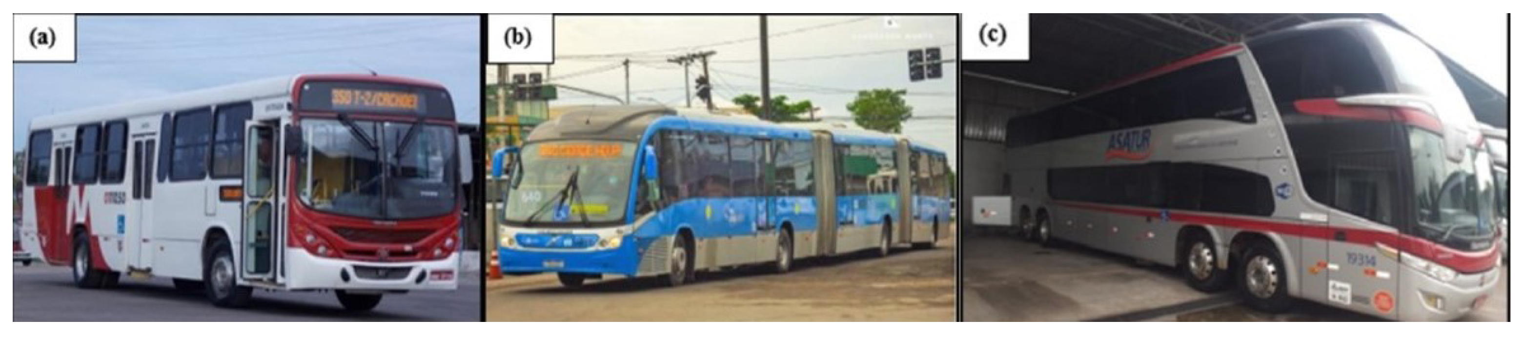
3. Materials and Methods
3.1. Defining and Implementing the Sample Model
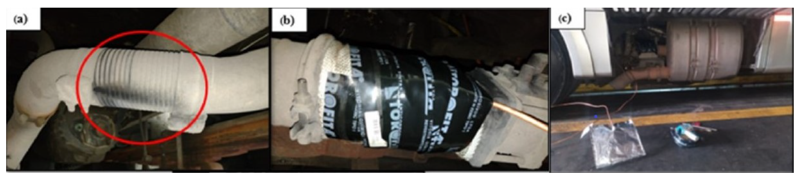
3.2. Experimental Procedure
3.3. Criteria and Reference Conditions Used for Gas Sampling
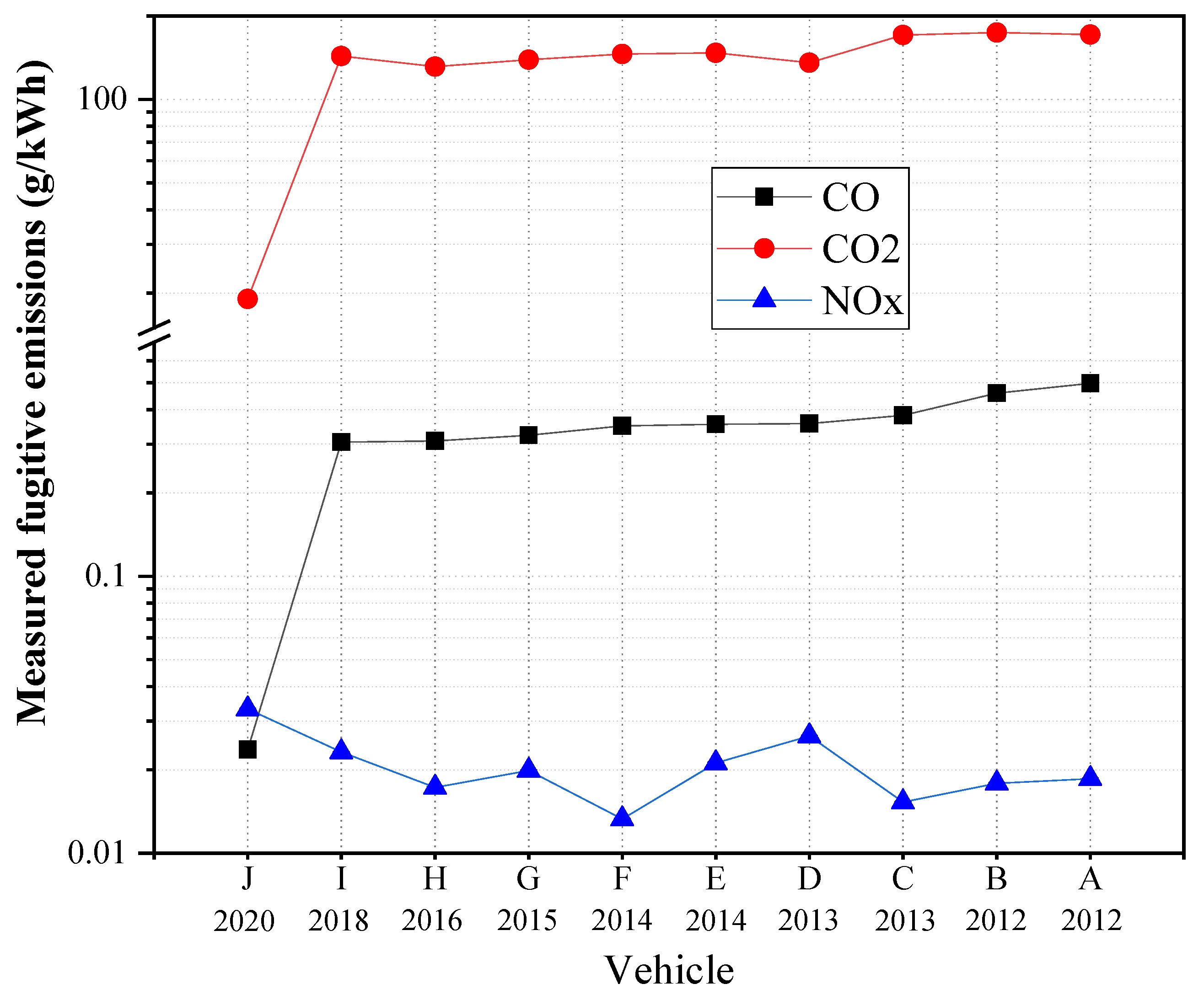
4. Results
Unit of Measure Transformation
5. Discussion
5.1. Influence of Mileage and Time Variables on Fugitive Emissions
5.1.1. Carbon Dioxide ()
5.1.2. Carbon Monoxide ()
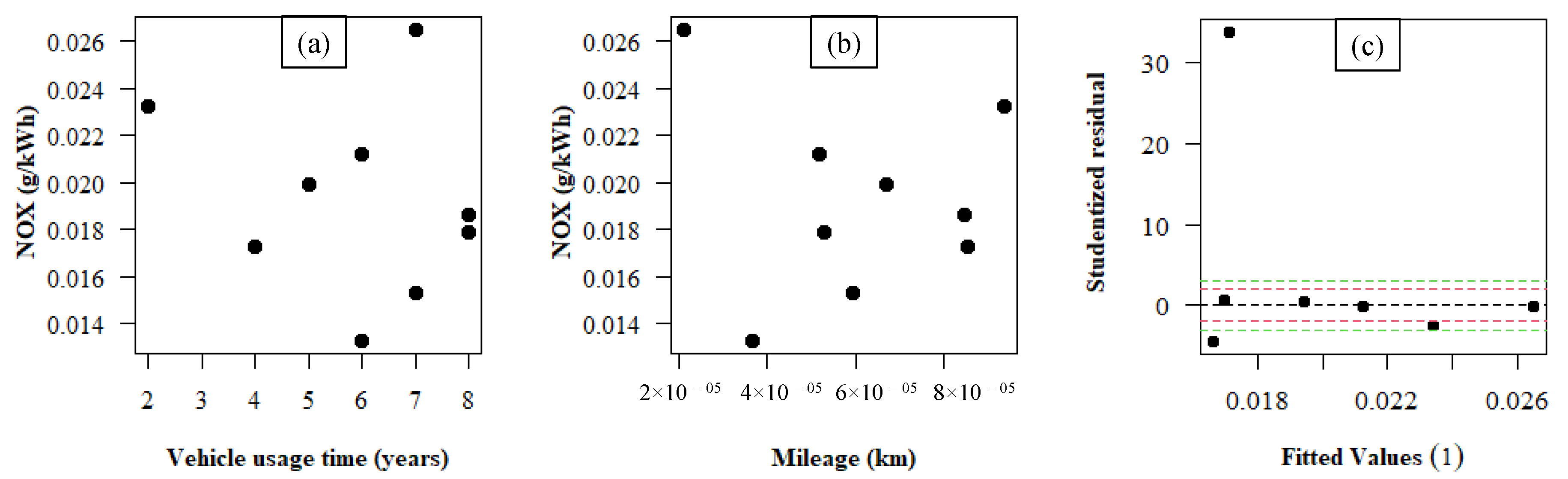
5.1.3. Nitrogen Oxides ()
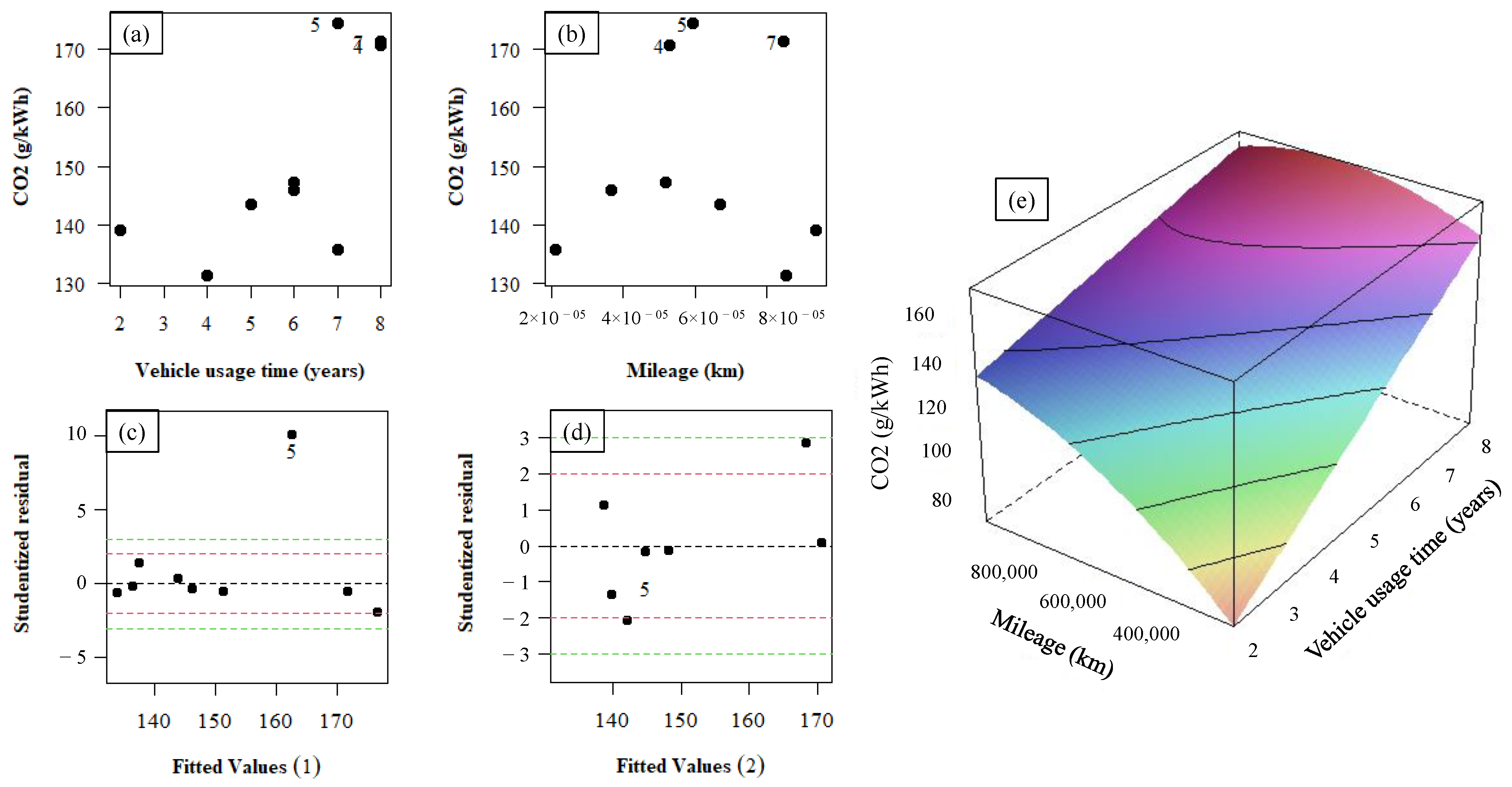
5.2. Trend Analysis Using Response Surface Methodology (RSM)
5.2.1. Carbon Dioxide
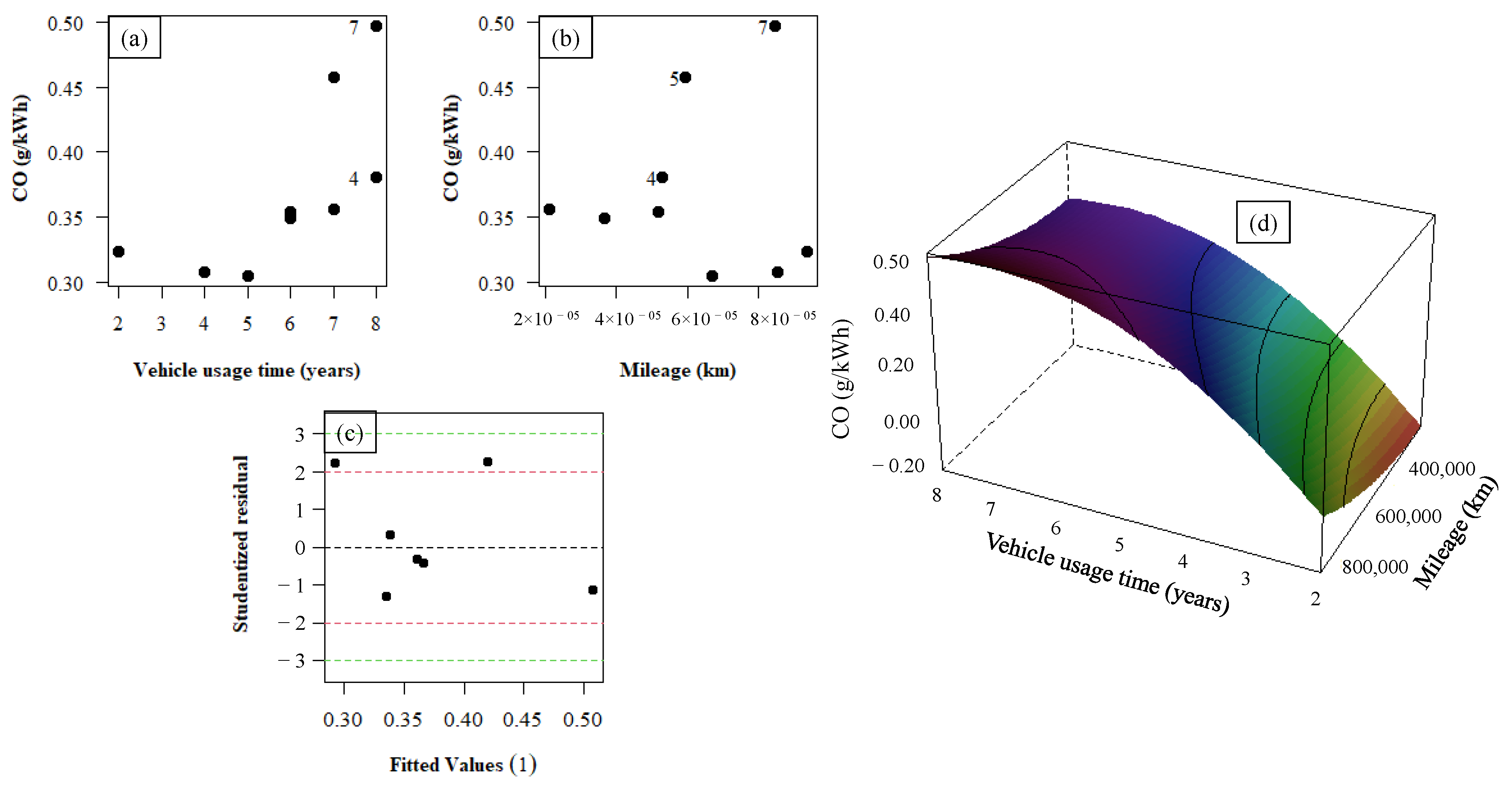
5.2.2. Carbon Monoxide ()
5.2.3. Nitrogen Oxide ()
6. Conclusions
Author Contributions
Funding
Informed Consent Statement
Acknowledgments
Conflicts of Interest
References
- IPCC. Global Warming of 1.5 °C: IPCC Special Report on Impacts of Global Warming of 1.5 °C above Pre-industrial Levels in Context of Strengthening Response to Climate Change, Sustainable Development, and Efforts to Eradicate Poverty, 1st ed.; Cambridge University Press: Cambridge, UK, 2022. [Google Scholar] [CrossRef]
- The United Nations. Report of the United Nations Conference on the Human Environment; Technical Report; The United Nations: Stockholm, Sweden, 1972. [Google Scholar]
- The United Nations. Report of the United Nations Conference on Environment and Development, Rio De Janeiro, Brazil, 3–14 June 1992; Volume 1, Resolutionsadopted By The Conference; Technical Report; The United Nations: Rio de Janeiro, Brazil, 1992. [Google Scholar]
- United Nations Climate Change. The Paris Agreement—UNFCCC; Technical Report; The United Nations: Paris, France, 2015. [Google Scholar]
- United Nations Climate Change. Greenhouse Gas Inventory Data—Time Series—Annex I—GHG total without LULUCF, in kt CO2 Equivalent. Available online: https://di.unfccc.int/ (accessed on 1 November 2022).
- The European Commission. Energy, Transport and Environment Statistics—2020 Edition; Technical Report; The European Commission, European Union: Stockholm, Sweden, 2020. [Google Scholar] [CrossRef]
- Intergovernmental Panel on Climate Change. Climate Change 2022: Mitigation of Climate Change; Technical Report; Working Group III Contribution to the Sixth Assessment Report of the Intergovernmental Panel on Climate Change; Cambridge University Press: Cambridge, UK; New York, NY, USA, 2022. [Google Scholar] [CrossRef]
- Intergovernmental Panel on Climate Change—IPCC. 2006 IPCC Guidelines for National Greenhouse Gas Inventories—Volume 1—General Guidance and Reporting Publications—IPCC-TFI, 2006. Chapter 8—Reporting Guidance and Tables. Available online: https://www.ipcc-nggip.iges.or.jp/public/2006gl/vol1.html (accessed on 1 November 2022).
- Intergovernmental Panel on Climate Change. Climate Change 2022: Impacts, Adaptation and Vulnerability; Technical Report; Working Group II Contribution to the Sixth Assessment Report of the Intergovernmental Panel on Climate Change; Cambridge University Press: Cambridge, UK; New York, NY, USA, 2022. [Google Scholar] [CrossRef]
- Laconde, T. Fugitive emissions: A blind spot in the fight against climate change. In Climate Chance—2018 Annual Report, Global Observatory On Non-State Climate Action; Climate Chance Association: Rue du Faubourg Saint-Antoine, Paris, 2018; Available online: https://www.climate-chance.org/en/2018report/ (accessed on 1 November 2022).
- Solazzo, E.; Crippa, M.; Guizzardi, D.; Muntean, M.; Choulga, M.; Janssens-Maenhout, G. Uncertainties in the Emissions Database for Global Atmospheric Research (EDGAR) emission inventory of greenhouse gases. Atmos. Chem. Phys. 2021, 21, 5655–5683. [Google Scholar] [CrossRef]
- Effiong, M.O.; Okoye, C.U.; Nweze, N.J. Sectoral contributions to carbon dioxide equivalent emissions in the nigerian economy. Int. J. Energy Econ. Policy 2019, 10, 456–463. [Google Scholar] [CrossRef] [Green Version]
- Hmiel, B.; Petrenko, V.V.; Dyonisius, M.N.; Buizert, C.; Smith, A.M.; Place, P.F.; Harth, C.; Beaudette, R.; Hua, Q.; Yang, B.; et al. Preindustrial 14CH4 indicates greater anthropogenic fossil CH4 emissions. Nature 2020, 578, 409–412. [Google Scholar] [CrossRef] [PubMed]
- United Nations Framework Convention on Climate Change—UNFCCC. Measurements for Estimation of Carbon Stocks—In Afforestation and Reforestation Project Activities under the Clean Development Mechanism—A Field Manual, 1st ed.; Platz der Vereinten Nationen: Bonn, Germany, 2015; Available online: http://www.unfccc.int (accessed on 1 November 2022).
- Singh, A.; Unnikrishnan, S.; Naik, M.; Sayanekar, S. CDM implementation towards reduction of fugitive greenhouse gas emissions. Environ. Dev. Sustain. 2019, 21, 569–586. [Google Scholar] [CrossRef]
- Nogueira, T.; Dominutti, P.A.; Vieira-Filho, M.; Fornaro, A.; Andrade, M.d.F. Evaluating Atmospheric Pollutants from Urban Buses under Real-World Conditions: Implications of the Main Public Transport Mode in São Paulo, Brazil. Atmosphere 2019, 10, 108. [Google Scholar] [CrossRef] [Green Version]
- The European Environment Agency (EEA). EMEP/EEA Air Pollutant Emission Inventory Guidebook—European Environment Agency; Publication Office of the European Union: Luxembourg, 2019. [CrossRef]
- Savickas, D.; Steponavičius, D.; Špokas, L.; Saldukaitė, L.; Semenišin, M. Impact of Combine Harvester Technological Operations on Global Warming Potential. Appl. Sci. 2021, 11, 8662. [Google Scholar] [CrossRef]
- Soares, P.H.; Monteiro, J.P.; Freitas, H.F.; Zenko Sakiyama, R.; Andrade, C.M. Platform for monitoring and analysis of air quality in environments with large circulation of people. Environ. Prog. Sustain. Energy 2018, 37, 2050–2057. [Google Scholar] [CrossRef]
- Soares, P.H.; Monteiro, J.P.; de Freitas, H.F.S.; Ogiboski, L.; Vieira, F.S.; Andrade, C.M.G. Monitoring and Analysis of Outdoor Carbon Dioxide Concentration by Autonomous Sensors. Atmosphere 2022, 13, 358. [Google Scholar] [CrossRef]
- Official Journal of the European Union. Regulation (EC) No 715/2007 of the European Parliament and of the Council of 20 June 2007. Doc ID: L:2007:171:TOC. Available online: https://eur-lex.europa.eu (accessed on 1 November 2022).
- Jenkins, D.G.; Quintana-Ascencio, P.F. A solution to minimum sample size for regressions. PLoS ONE 2020, 15, e0229345. [Google Scholar] [CrossRef] [PubMed] [Green Version]
- Yoo, H.; Lee, J.W. Sample size calculation based on discrete Weibull and zero-inflated discrete Weibull regression models. Commun. Stat.—Simul. Comput. 2022, 51, 7180–7193. [Google Scholar] [CrossRef]
- National Service Center for Environmental Publications (NSCEP). Protocol for Equipment Leak Emission Estimates; Report EPA-453/R-95-017; NSCEP: Research Triangle Park, NC, USA, 1995.
- Hennigan, S. Method 21 monitors fugitive emissions. Environ. Prot. 1993, 4, 22–31. Available online: https://www.osti.gov/biblio/249852 (accessed on 1 November 2022).
- Wilson, A. New Optical Gas-Imaging Technology for Quantifying Fugitive-Emission Rates. J. Pet. Technol. 2016, 68, 78–79. [Google Scholar] [CrossRef]
- Abdel-Moati, H.; Morris, J.; Zeng, Y.; Kangas, P.; McGregor, D. New Optical Gas Imaging Technology for Quantifying Fugitive Emission Rates; OnePetro: Doha, Qatar, 2015. [Google Scholar] [CrossRef]
- Asiamah, N.; Conduah, A.K.; Eduafo, R. Social network moderators of the association between Ghanaian older adults’ neighbourhood walkability and social activity. Health Promot. Int. 2021, 36, 1357–1367. [Google Scholar] [CrossRef] [PubMed]
- Maas, R.P.P.W.M.; Teerenstra, S.; Toni, I.; Klockgether, T.; Schutter, D.J.L.G.; van de Warrenburg, B.P.C. Cerebellar Transcranial Direct Current Stimulation in Spinocerebellar Ataxia Type 3: A Randomized, Double-Blind, Sham-Controlled Trial. Neurotherapeutics 2022, 19, 1259–1272. [Google Scholar] [CrossRef] [PubMed]
- Yurdakoş, K.; Sarihan, M. Irrational use of medicines: The magnitude of economic loss due to wasted medicines that cannot be prescribed, sold and used in an instant optimized manner. Mersin Üniv. Sağlık Bilim. Derg. 2022, 15, 517–530. [Google Scholar] [CrossRef]
- VOLVO do Brasil. Volvo B270F Charter Specifications. 2022. Available online: https://www.volvobuses.com/br/Rodoviario/b270f-fretamento/specifications.html (accessed on 1 October 2022).
- VOLVO do Brasil. Volvo B340M Charter Specifications. 2022. Available online: https://www.volvobuses.com/br/Urbano/b340m-articulado-biarticulado/specifications.html (accessed on 1 October 2022).
- VOLVO do Brasil. Volvo B11R Charter Specifications. 2022. Available online: https://www.volvobuses.com/en/coaches/chassis/volvo-b11r/specifications.html (accessed on 1 October 2022).
- Vergel-Ortega, M.; Valencia-Ochoa, G.; Duarte-Forero, J. Experimental study of emissions in single-cylinder diesel engine operating with diesel-biodiesel blends of palm oil-sunflower oil and ethanol. Case Stud. Therm. Eng. 2021, 26, 101190. [Google Scholar] [CrossRef]
- Ağbulut, U.; Sarıdemir, S.; Albayrak, S. Experimental investigation of combustion, performance and emission characteristics of a diesel engine fuelled with diesel–biodiesel–alcohol blends. J. Braz. Soc. Mech. Sci. Eng. 2019, 41, 389. [Google Scholar] [CrossRef]
- Kopseak, H.; Pandur, Z.; Bačić, M.; Zec̆ić, u.; Nevec̆erel, H.; Lepoglavec, K.; S̆us̆njar, M. Exhaust Gases from Skidder ECOTRAC 140 V Diesel Engine. Forests 2022, 13, 272. [Google Scholar] [CrossRef]
- Soca-Cabrera, J.R. Diesel engine emissions off road. Case Volskwagen ADG 1.9 L SDI. Rev. Cienc. Técnicas Agropecu. 2020, 29, 15–23. [Google Scholar]
- R Core Team. R: A Language and Environment for Statistical Computing; R Foundation for Statistical Computing: Vienna, Austria, 2021. [Google Scholar]
- Global Monitoring Laboratory. In Carbon Cycle Greenhouse Gases; 2023. Available online: https://gml.noaa.gov/ccgg/ (accessed on 18 February 2023).
- Baumgarten, C. Mixture Formation in Internal Combustion Engine; Heat, M.T., Ed.; Springer: Berlin/Heidelberg, Germany, 2006. [Google Scholar] [CrossRef]
- Adão, W.B.; Cancino, L.R. Spray Behavior on Compression Ignition Internal Combustion Engines: A CFD Analysis of Cavitation in the Fuel Injector. In Proceedings of the COBEM 2019—25th ABCM International Congress of Mechanical Engineering, Uberlândia, Brazil, 20–25 October 2019; p. COB–2019–2161. [Google Scholar]
- Henschel, J.A., Jr.; Cancino, L.R. Numerical Analysis of Fuel Spray Angle on the Operating Parameters in a Locomotive Diesel Engine. In Proceedings of the COBEM 2019—25th ABCM International Congress of Mechanical Engineering, Uberlândia, Brazil, 20–25 October 2019; p. COB–2019–1642. [Google Scholar]
- Rotter, D.V.; Hackbarth, G.Z.; Henschel, J.A., Jr.; Cancino, L.R. Spray and Combustion Behavior in a Locomotive Engine Using Diesel/Biodiesel Blends: A CRFD Analysis. In Proceedings of the COBEM 2021—26th International Congress of Mechanical Engineering, Online, 22–26 November 2021; p. COB–2021–0706. [Google Scholar]


| Production | Mileage | Rotation | Power | Gas Sample | Engine * | Wall | Transport |
|---|---|---|---|---|---|---|---|
| Year | (km) | (rpm) | (cv/kW) | Collection Time (s) | Temperature (°C) | Temperature (°C) | Category |
| 2014 | 518,640 | 1700 | 340/250.07 | 664 | 93.1 | 175.0 | Urban |
| 2014 | 367,100 | 1700 | 340/250.07 | 721 | 92.4 | 155.0 | Urban |
| Production | Mileage | Rotation | Power | Gas Sample | Engine * | Wall | Transport |
|---|---|---|---|---|---|---|---|
| Year | (km) | (rpm) | (cv/kW) | Collection Time (s) | Temperature (°C) | Temperature (°C) | Category |
| 2012 | 846,694 | 1700 | 270/198.58 | 788 | 87.0 | 110.0 | Urban |
| 2012 | 367,100 | 1700 | 270/198.58 | 602 | 86.0 | 103.7 | Urban |
| 2013 | 518,640 | 1700 | 270/198.58 | 540 | 88.0 | 106.0 | Urban |
| 2013 | 367,100 | 1700 | 270/198.58 | 781 | 85.0 | 104.6 | Urban |
| Production | Mileage | Rotation | Power | Gas Sample | Engine * | Pipeline Wall | Transport |
|---|---|---|---|---|---|---|---|
| Year | (km) | (rpm) | (cv/kW) | Collection Time (s) | Temperature (°C) | Temperature (°C) | Category |
| 2015 | 670,803 | 1700 | 450/330.97 | 660 | 96.0 | 137.0 | Road |
| 2016 | 856,794 | 1700 | 450/330.97 | 664 | 92.0 | 104.0 | Road |
| 2018 | 938,933 | 1700 | 450/330.97 | 605 | 94.0 | 152.0 | Road |
| 2020 | 93,449 | 1700 | 450/330.97 | 721 | 91.8 | 132.0 | Road |
| Vehicle | Mass (kg) | Time (s) | Mass Flow Rate (kg/s) |
|---|---|---|---|
| A | 0.011 | 788 | 1.396 |
| B | 0.017 | 540 | 3.148 |
| C | 0.027 | 602 | 4.485 |
| D | 0.015 | 781 | 1.921 |
| E | 0.029 | 664 | 4.637 |
| F | 0.023 | 721 | 3.190 |
| G | 0.024 | 605 | 3.967 |
| H | 0.090 | 664 | 1.355 |
| I | 0.011 | 660 | 1.667 |
| J | 0.012 | 721 | 1.664 |
| Vehicle | Model | Year | Mileage | * | * | * |
|---|---|---|---|---|---|---|
| (km) | (g/kWh) | (g/kWh) | (g/kWh) | |||
| A | B270F | 2012 | 846,694 | 4.97 ± 4.9 | 171.3 ± 1.7 | 1.86 ± 9.2 |
| B | B270F | 2012 | 528,923 | 4.58 ± 4.5 | 174.5 ± 1.7 | 1.79 ± 8.9 |
| C | B270F | 2013 | 595,771 | 3.81 ± 3.8 | 170.7 ± 1.7 | 1.53 ± 7.6 |
| D | B270F | 2013 | 210,814 | 3.56 ± 3.5 | 135.8 ± 1.3 | 2.65 ± 1.3 |
| E | B340M | 2014 | 518,640 | 3.54 ± 3.5 | 147.2 ± 1.4 | 2.12 ± 1.0 |
| F | B340M | 2014 | 367,100 | 3.49 ± 3.4 | 145.9 ± 1.4 | 1.33 ± 6.6 |
| G | B450R | 2015 | 670,803 | 3.23 ± 3.2 | 138.9 ± 1.3 | 1.99 ± 9.9 |
| H | B450R | 2016 | 856,794 | 3.08 ± 3.0 | 131.3 ± 1.3 | 1.73 ± 8.6 |
| I | B450R | 2018 | 938,933 | 3.05 ± 3.0 | 143.4 ± 1.4 | 2.32 ± 1.1 |
| J | B450R | 2020 | 93,449 | 2.37 ± 2.3 | 19.0 ± 0.2 | 3.32 ± 1.6 |
| Vehicle | Model | Year | Mileage | |
|---|---|---|---|---|
| (km) | (g/kWh) | |||
| A | B270F | 2012 | 846,694 | 171.3 ± 1.7 |
| B | B270F | 2013 | 595,771 | 174.5 ± 1.7 |
| C | B270F | 2012 | 528,923 | 170.7 ± 1.7 |
| D | B270F | 2013 | 210,814 | 135.8 ± 1.3 |
| E | B340M | 2014 | 518,640 | 147.2 ± 1.4 |
| F | B340M | 2014 | 367,100 | 145.9 ± 1.4 |
| G | B450R | 2018 | 938,933 | 138.9 ± 1.3 |
| H | B450R | 2016 | 856,794 | 131.3 ± 1.3 |
| I | B450R | 2015 | 670,803 | 143.4 ± 1.4 |
| J | B450R | 2020 | 93,449 | 19.0 ± 0.2 |
| Vehicle | Model | Year | Mileage | |
|---|---|---|---|---|
| (km) | (g/kWh) | |||
| A | B270F | 2012 | 846,694 | 4.97 ± 4.97 |
| B | B270F | 2013 | 595,771 | 4.58 ± 4.58 |
| C | B270F | 2012 | 528,923 | 3.81 ± 3.81 |
| D | B270F | 2013 | 210,814 | 3.56 ± 3.56 |
| E | B340M | 2014 | 518,640 | 3.54 ± 3.54 |
| F | B340M | 2014 | 367,100 | 3.49 ± 3.49 |
| G | B450R | 2018 | 938,933 | 3.23 ± 3.23 |
| H | B450R | 2016 | 856,794 | 3.08 ± 3.08 |
| I | B450R | 2015 | 670,803 | 3.05 ± 3.05 |
| J | B450R | 2020 | 93,449 | 2.37 ± 2.37 |
| Vehicle | Model | Year | Mileage | |
|---|---|---|---|---|
| (km) | (g/kWh) | |||
| A | B270F | 2012 | 846,694 | 1.86 ± 9.29 |
| B | B270F | 2013 | 595,771 | 1.79 ± 8.96 |
| C | B270F | 2012 | 528,923 | 1.53 ± 7.63 |
| D | B270F | 2013 | 210,814 | 2.65 ± 1.33 |
| E | B12M | 2014 | 518,640 | 2.12 ± 1.06 |
| F | B12M | 2014 | 367,100 | 1.33 ± 6.64 |
| G | B450R | 2018 | 938,933 | 1.99 ± 9.95 |
| H | B450R | 2016 | 856,794 | 1.73 ± 8.63 |
| I | B450R | 2015 | 670,803 | 2.32 ± 1.16 |
| J | B450R | 2020 | 93,449 | 3.32 ± 1.66 |
Disclaimer/Publisher’s Note: The statements, opinions and data contained in all publications are solely those of the individual author(s) and contributor(s) and not of MDPI and/or the editor(s). MDPI and/or the editor(s) disclaim responsibility for any injury to people or property resulting from any ideas, methods, instructions or products referred to in the content. |
© 2023 by the authors. Licensee MDPI, Basel, Switzerland. This article is an open access article distributed under the terms and conditions of the Creative Commons Attribution (CC BY) license (https://creativecommons.org/licenses/by/4.0/).
Share and Cite
Caetano, A.C.; da Costa, A.M.S.; Janeiro, V.; Soares, P.H.; Cancino, L.R.; Andrade, C.M.G. Fugitive Emissions from Mobile Sources—Experimental Analysis in Buses Regulated by the Euro 5 Standard. Atmosphere 2023, 14, 613. https://doi.org/10.3390/atmos14040613
Caetano AC, da Costa AMS, Janeiro V, Soares PH, Cancino LR, Andrade CMG. Fugitive Emissions from Mobile Sources—Experimental Analysis in Buses Regulated by the Euro 5 Standard. Atmosphere. 2023; 14(4):613. https://doi.org/10.3390/atmos14040613
Chicago/Turabian StyleCaetano, Antonio C., Alexandre M. S. da Costa, Vanderly Janeiro, Paulo H. Soares, Leonel R. Cancino, and Cid M. G. Andrade. 2023. "Fugitive Emissions from Mobile Sources—Experimental Analysis in Buses Regulated by the Euro 5 Standard" Atmosphere 14, no. 4: 613. https://doi.org/10.3390/atmos14040613