1. Introduction
During vehicle operation different amounts of pollutants are emitted depending on the raw engine-out emissions and the efficiency of the catalytic converter. These pollutants, such as nitrogen oxides (NO
), have negative effects on human health and the environment. Previous studies from [
1,
2] have found excessive pollutant concentrations in many European cities.
Vehicle emissions testing is currently performed prior to homologation by installing a portable emission measurement system (PEMS) in the test vehicle as well as in a laboratory on a chassis dynamometer while the vehicle is driven on a specified test cycle. Remote Emission Sensing (RES) has recently attracted interest, allowing a large number of vehicles to be tested under real-world conditions. Ref. [
3] explains how to determine real-world emissions from passenger vehicles using RES and [
4] elaborates on how emission factors (e.g., gram pollutant/km) can be derived.
A RES device is placed directly next to the road with the test vehicle completely separated from the emission test facility. Besides the possibility to characterize the vehicle fleet through statistic evaluations, another idea behind RES is to identify vehicle models with excessive emissions under real-world conditions [
5]. A RES device essentially measures the ratio
, but there still exist many uncertainties in the measured data provided by the RES device when operating at different conditions. Therefore, further investigation of the limitations of the measurement systems is needed. For assessing the reliability of RES devices, the turbulent flow behavior of the vehicle wake and its influence on the exhaust plume must be understood. Therefore, in the present work, Computational Fluid Dynamics (CFD) is used to simulate the flow around the vehicle, and to analyze the exhaust plume dispersion in the vehicle wake.
In general, the flow around a vehicle is turbulent due to high Reynolds numbers. The nature of turbulence is always unsteady, three-dimensional and chaotic, such that mixing is strongly enhanced. Especially in the transverse directions (perpendicular to the main flow direction) a strong exchange of momentum, heat and species prevails. In complex flows several types of turbulence often occur side by side. For example, in the flow around a vehicle turbulent boundary layers (directly at the front and side contours) but also detached free shear layers and wake flows (downstream the rear of the vehicle and the wing mirrors) are present. In the following, different approaches to simulate a turbulent flow are discussed.
For direct numerical simulations (DNS) no turbulence modeling assumptions are made, but a numerical solution of the Navier-Stokes equations describing all flow details is performed. The turbulent flow is thus computed in detail, so that all turbulent scales must be resolved. Therefore, the computation time for a given 3D flow roughly scales with , which is why DNS is in general not suited for practical simulations.
Large eddy simulations (LES) solve the spatially filtered Navier-Stokes equations. Ideally, all turbulence elements larger than the selected spatial filter width are resolved. The effect of the unresolved smaller turbulence elements must therefore be approximated by a suitable turbulence model. LES is a good compromise, especially for free shear flows, where the computational cost of LES is only weakly dependent on the Reynolds number (
) [
6,
7]. However, the cost required for a wall-resolved LES scales with
, similar to direct numerical simulation (DNS) [
8,
9].
Nevertheless, DNS and (wall-resolved) LES are computationally too expensive for the flow around a vehicle (
). Therefore, in the present work, the Unsteady Reynolds-Averaged Navier-Stokes (URANS) equations are used. In this way, turbulent scales are modeled, but large coherent vortex structures are resolved. These structures/eddies are coherent because they occur with some regularity. For this reason URANS is considered to be an eddy-resolving method [
10]. This implies that the detachment of the flow around the vehicle creates not only a large number of small turbulent eddies, but also recurring large eddies. However, all turbulent fluctuations of the flow are treated by the turbulence model. In contrast to URANS, RANS would not be able to resolve the unsteady coherent structures, since it is not time-resolving and thus only describes a statistically stationary state. After all, the results of both, URANS and RANS can be seen as expected values of the mean flow, since they rely on statistics. However, URANS has proven to perform better and provides a more accurate expectation of the mean flow [
11].
Previous investigations have already studied the exhaust plume using different turbulence modeling approaches. Ref. [
12] investigated pollutant dispersion in a road tunnel, where the effect of moving vehicle wakes was of particular interest. Ref. [
13] simulated vehicular pollutant dispersion in the atmospheric environment using a RANS model and compared the results with measurements. However, they did not include a vehicle model in their simulation, but simulated the exhaust plume dispersion downstream the exhaust tailpipe for different ambient conditions. Ref. [
14] investigated carbon monoxide dispersion of a realistic vehicle model by combining the Lattice Boltzmann Method with the LES. Furthermore, ref. [
15] looked into near-field dynamics and plume dispersion behind a heavy-duty vehicle using wall-modeled LES. They also drew first conclusions for on-road RES measurements, e.g., the sampling duration of an individual measurement. In addition, ref. [
16] simulated vehicle emission dispersion with wall-modeled LES. For a simplified vehicle model, they investigated different parameters regarding RES and proposed possible improvements to the accuracy of a RES device. Moreover, ref. [
17] provides a good overview of recent CFD studies investigating pollutant dispersion.
To provide additional insights on the exhaust plume dispersion downstream a realistic vehicle and how this affects an on-road RES measurement, in the present work, a parameter study deepening and extending the one by [
18] was carried out to relate various properties of the exhaust plume to the given circumstances. Since the parameter study led to numerous simulations, this was another reason URANS was chosen instead of LES or hybrid LES/RANS [
19]. To the best of our knowledge, the pollutant dispersion behavior has never been analyzed with respect to the currently available RES technologies, as it is done in this paper. An additional novelty of this work is the systematic investigation of the influence of different parameters. The chosen parameters are, on one hand, vehicle-related characteristics such as velocity as well as the position and orientation of the exhaust tailpipe. Additionally, wind is included in the study as a general external effect, distinguishing between orientation and wind velocity. Furthermore, an analysis on how a vehicle upstream affects the exhaust plume dispersion of a vehicle further downstream is given.
The remainder of the paper is organized as follows. The details of the URANS solver, the computational domain/mesh as well as RES are explained in
Section 2. The described solver is used to simulate flow around the vehicle at different driving and ambient conditions. The results from the parameter study are presented and discussed in
Section 3.
Section 4 concludes this paper.
2. Methodology
The following describes the setup of a simulation environment in OpenFOAM for the flow around a vehicle, which is emitting exhaust gases. Thus, temperature as well as density vary in space and time, since the exhaust is a high temperature multicomponent mixture. Therefore, the Navier-Stokes-Fourier system of equations containing the conservation equations of mass, momentum, energy and species are considered to simulate the mentioned flow problem. For the sake of simplicity, it is referred to these equations as the Navier-Stokes equations.
2.1. URANS Governing Equations
Even though the maximum Mach number is
and thus the fluid is considered incompressible, the Navier-Stokes equations are written in a low-speed form, where the density varies, especially in the near exhaust region due to high temperature gradients. Reynolds-averaging the Navier-Stokes equations and introducing the density-weighted Favre-average
as a mathematical simplification leads to a closure problem. Thus, the eddy viscosity hypothesis for momentum,
species,
and enthalpy,
is implemented according to [
20] in order to reduce the number of unknowns to one (
). The eddy viscosity
is not a fluid property, but a flow quantity that must be modeled. There exist a large number of models for the eddy viscosity, which can be classified according to the number of additional transport equations that need to be solved. In this work, the two-equation
k-
SST model as proposed by [
21] is used. This turbulence model provides a better prediction of flow separation than most RANS models. It has the ability to account for the transport of the principal shear stress in adverse pressure gradient boundary layers. Therefore, it is well suited for aerodynamic flows [
22]. Incorporating all these assumptions into the governing equations leads to the URANS equations, where the equation for conservation of mass is given by
Momentum conservation in the case of URANS can be written as
and in addition, the energy equation yields
where the quantity
is the diffusive flux of species
k, and
is the total energy and
describes the total enthalpy.
E and
H both include the turbulent kinetic energy
k. It has to be mentioned that the buoyancy term is treated explicitly in the momentum and energy equation and is not contributing to the pressure, i.e.,
is not
. Together with the Reynolds-averaged species equation,
the continuity equation can be defined as the sum of all species equations and the set of URANS equations is complete. The eddy viscosity as well as eddy mass and heat diffusivity are combined with the molecular counterpart as
with the Schmidt-numbers being
and
, as well as the Prandtl-numbers defined as
.
Finally, as an equation of state, the ideal gas law
is considered, where
is the molecular weight of species
k and
is the universal gas constant.
Implementation
The above described equations are implemented in the open source CFD platform OpenFOAM, making use of its existing solvers and various functionalities [
23,
24]. The PISO (Pressure Implicit with Splitting of Operators) algorithm is chosen to iteratively solve the coupled equations. Therefore, Equation (
5) is not solved for the density but used to construct a pressure-poisson equation as presented in [
25]. The PISO algorithm follows an iterative procedure, which can be broken down to the following steps for each time step:
- 1.
Momentum prediction: solve the momentum equation with pressure field from previous time step.
- 2.
Pressure solution: solve the pressure equation to receive pressure field update.
- 3.
Velocity correction: correct velocity based on updated pressure field and momentum equation.
Steps 2 and 3 need to be repeated until convergence.
- 4.
Calculate density based on the ideal gas law.
Thus, mass conservation is still ensured (through construction of the pressure-poisson equation) and the simulation runs very stable for low-Mach numbers. The time step is obtained by the Courant-Friedrichs-Lewy (CFL) condition and continuously updated to conform with
Thus, an upper limit of
is deployed, and
is calculated according to Equation (
15). On average, the time step is in the order of magnitude of
s once convergence is reached.
Additionally, parallel computing which is an in-built feature of OpenFOAM is implemented as domain decomposition, in which the geometry and associated fields are broken into pieces and allocated to separate processors. The process of parallel computation involves: decomposition of mesh and fields; running the application in parallel; post-processing the decomposed case. The parallel computations use the public domain openMP of the standard message passing interface (MPI).
Implicit Euler is chosen for time integration, gradient and laplacian terms are discretized with second order central schemes and limited linear differencing is used for the divergence terms [
26]. A geometric-algebraic multi-grid (GAMG) method is employed to solve the symmetric equation system of pressure, whereas the stabilized preconditioned bi-conjugate gradient (PBiCGStab) method is used to solve the asymmetric equation systems of all other variables. Tolerances are chosen to be
, such that the iterative solver stops when the residual falls below the solver’s tolerance.
All simulations were performed on the computational architecture described in
Table A2.
2.2. Computational Domain and Boundary Conditions
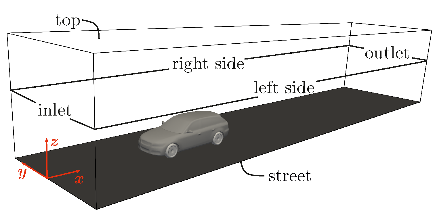
The computational domain shown in
Figure 1 is created to simulate the flow around the vehicle and, in particular, the dispersion of pollutants in the vehicle wake. A total size of
(35, 16, 8) m is selected. In order to simulate the flow around a vehicle in an open-road environment, an even bigger domain, as also suggested by [
27], could be used. However, these dimensions have been proven appropriate, while the lateral boundary conditions are showing a small influence on the flow. In fact, enlarging the domain just produced a higher number of cells but showed an insignificant deviation from results obtained with smaller dimensions. For instance, the cut plane concentration integrals downstream the vehicle, as discussed in
Section 2.5 deviated less than 2%. The computational cost, however, increased by more than 27%.
As a vehicle, the DrivAer body, specially developed for aerodynamic simulations by [
28], was chosen, because it is modeled in great detail and is thus close to a real vehicle. Furthermore, the shape of the vehicle is very typical for an average vehicle on European roads. The modular design also offers the possibility to simulate different rear end geometries. The geometry can be found in [
29].
At the inlet, Dirichlet boundary conditions (BCs) for velocity, species, temperature and turbulent variables are applied. Inlet velocity points, species mass fractions and temperature are set to atmospheric conditions and the turbulent variables k and are based on a turbulence intensity of 1% and an eddy-viscosity ratio of . Therefore, where is the face value of the above mentioned flow and turbulent variables and the respective reference value. Regarding the pressure, Neumann BCs (i.e., where is the pressure in this case and is the boundary face normal vector) are applied at all boundaries except at the outlet, where the atmospheric pressure is prescribed. For all other variables Neumann BCs are employed. Slip BCs (, where ⊥ is the normal component) are used for the velocity at the right/left sides and at the top. Regarding k and , wall functions are applied at every solid wall (street, vehicle and wheels) whereas Neumann BCs are used for the outer boundaries (right/left side, top). Additionally, Neumann BCs are considered for species mass fractions and temperature. At the vehicle surface no-slip ( m/s) conditions are used whereas the street has the same stream-wise velocity as the inlet ( m/s) such that the movement of the vehicle relative to the street is captured correctly. The wheels have a rotational velocity obeying the aforementioned velocity of the street and radius r of the wheel, i.e., .
2.3. Computational Mesh
Since OpenFOAM is based on the finite-volume-method for unstructured meshes, such a mesh needs to be created. Therefore, the meshing utility
snappyHexMesh supplied with OpenFOAM is used to create hexahedra-dominant meshes. The mesh approximately conforms to the surface by iteratively refining a starting mesh and morphing the resulting split-hexahedra mesh to the surface [
24].
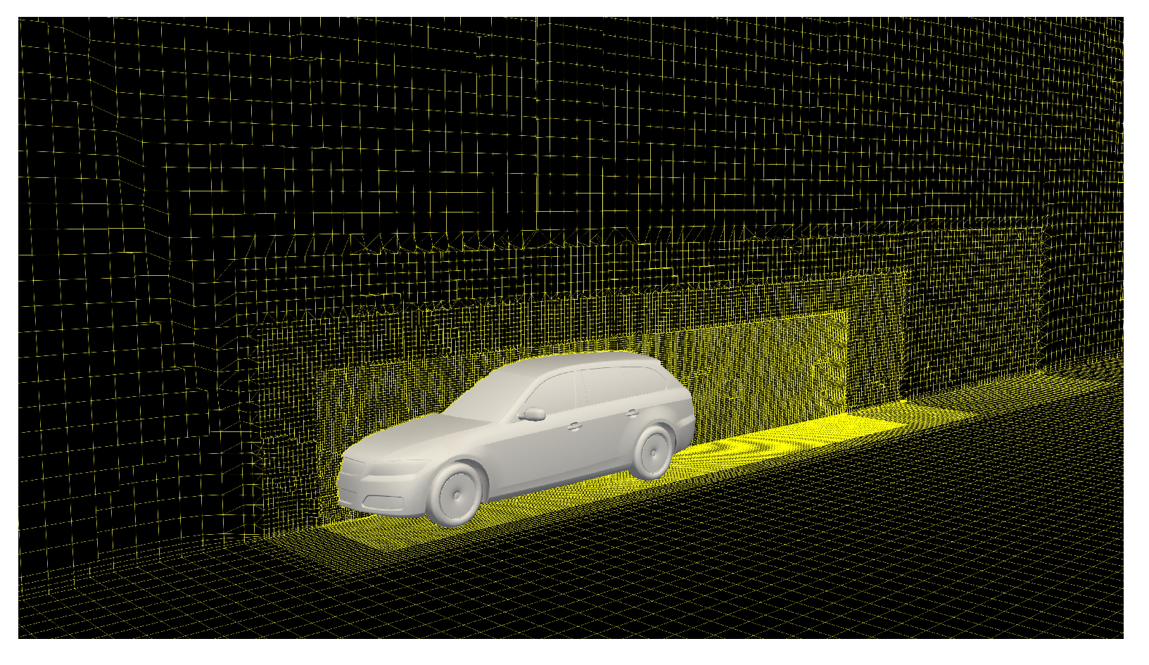
When creating the computational mesh, particular attention was paid to a balance between necessary computational time and accuracy in the sense of a sufficiently high resolution. For the investigation of several influencing parameters, more than 100 simulations were performed; therefore the computation time per simulation had to be limited. After several iterations of the mesh generation, the mesh shown in
Figure 2 was obtained and selected.
Two further aspects were of particular concern during the mesh generation. On one hand the dimensionless wall distance at the nearest grid points was enforced to be between 30 and 300. Thus wall functions are used to estimate the mean velocity at the first grid points which serve as a Dirichlet BC for the numerical calculation of the turbulent kinetic energy k as well as the turbulent dissipation rate . The other option would be to resolve the boundary layer down to the viscous sub-layer () and not rely on wall functions. However, this would result in a large number of grid cells, which would increase the computational time enormously, but in turn would not substantially improve the accuracy of the contaminant dispersion. Therefore, the wall functions were used to save computational time. In order to ensure a sufficiently high resolution of the flow near the wall, prism layers were added around the vehicle and on the road. For the description of the dispersion, on the other hand, a more precise resolution was chosen in the vehicle wake. Especially in the near vehicle wake, the resolution has been significantly increased and then gradually decreased with increasing distance from the vehicle. The computational mesh described so far served as the basis for most of the simulations, but changes have also been made for the simulations with crosswind. Due to the increased velocity caused by the additional wind velocity under the influence of different wind incidence angles, the mesh was extra refined and the computational domain was enlarged.
Mesh Independence Study
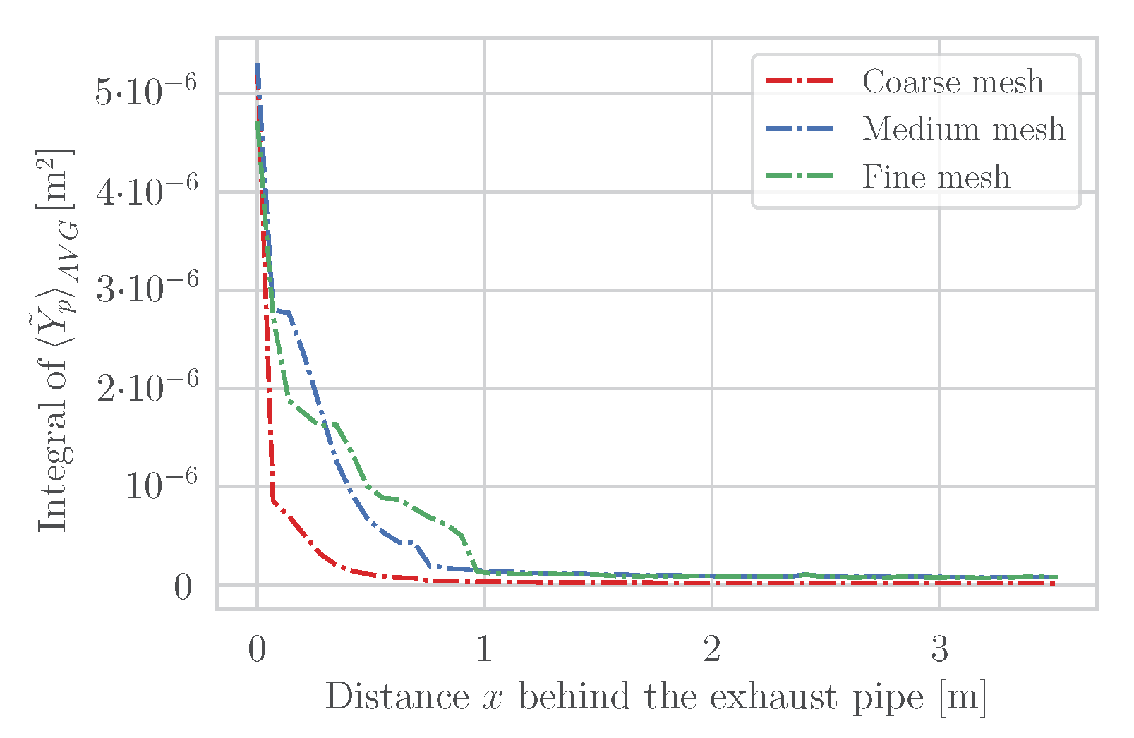
Mesh independence is of major concern in CFD. Therefore, three different meshes were tested under the same conditions. URANS simulations were performed till the residuals of the time-averaged pollutant mass fraction (
) dropped below
. The integrals of pollutant mass fraction in the
-planes downstream the tailpipe exit are compared in
Figure 3 (see also Equation (
19)). Here, the pollutant is averaged over 20 periods to account for the time-dependent vortex shedding.
The coarse mesh consists of 1,252,409 cells, the medium mesh of 2,753,191 cells and the fine mesh of 4,252,509 cells. The increase in cells from coarse to fine is mainly caused by the enhanced refinement level in the wake of the vehicle, since the pollutant dispersion in this area is of particular interest. The number of prism layers as well as the cubic base cell size of 20 cm in the free-stream regions is kept constant. Gradual refinement leads to a cubic cell size of 2.5 cm, 1.25 cm and 0.625 cm in the near-wake region for the coarse, medium and fine meshes, respectively.
Figure 3 depicts how the pollutant disperses fastest on the coarse mesh and slowest on the fine mesh. The medium mesh over-predicts the pollutant mass fraction in the first 0.3 m and slightly under-predicts further downstream. However, the discrepancy between the medium and fine mesh results is rather small. Thus, while mesh independence is not fully achieved by choosing the medium mesh, it is small enough to justify its use; note that the computational cost with the fine mesh is substantially higher than the one with the medium mesh. For this reason, and due to the fact that numerous simulations needed to be conducted as part of a parameter study, the medium mesh provided a good compromise. Details of the final mesh are listed in
Table A1.
2.4. Experimental Validation
The above described numerical model has been validated against experimental data. Refs. [
28,
30] studied the DrivAer body in the wind tunnel at different Reynolds numbers. For this purpose, drag coefficients
at these Reynolds numbers with and without ground simulation were determined using the numerical model and computational mesh as discussed earlier. Therefore, the simulations are aimed to resemble the experimental setups.
Table 1 compares the drag coefficients from simulation and experiment.
The discrepancy between the results of simulation and experiment is very low in case of
considering a high-
turbulence model was used. Nevertheless, a higher deviation of the results from simulation to experiment can be found for
without ground simulation. However, since the agreement between simulation and experiment is very good in case of higher Reynolds numbers, it is also possible that the different experimental setup causes the higher discrepancy. Ref. [
30] uses a 1:4 scale model of the DrivAer body while [
28] resorts to a 1:2.5 scale model and thus a different wind tunnel design. Hence, the accuracy has proven to be appropriate for subsequent pollutant dispersion simulations.
2.5. Remote Emission Sensing
Remote Emission Sensing measures exhaust emissions through absorption spectroscopy without affecting traffic. Absorption spectroscopy is a technique based on the differential absorption at a specific wavelength of a laser, UV or IR beam through a sample, in this case the exhaust plume.
There exist two main technologies on the market: The Fuel Efficiency Automobile Test (FEAT), such as distributed by [
31] and the Emission Detector and Reporting (EDAR) incorporated in the RES system by [
32].
FEAT places the emission sensors next to the road and uses a horizontal light beam at a fixed height above the road. The light is reflected back from a mirror on the other side of the road and focused on a detector. In this work, we refer to this instrument as the line-measurement instrument.
The detector of EDAR is positioned above the road. It uses a vertical laser sheet which is reflected by a special strip on the road surface back to the detector. We refer to this instrument as the plane-measurement instrument.
To determine the fuel-specific emission factor, the concentration of the individual species is measured in the form of a voltage. Knowing the absorption
and the molar attenuation coefficient
of the species
, the concentration
c of species
can be determined from the Beer-Lambert law,
Assuming that the exhaust plume is well mixed, the optical path length
l can be considered to be the same for each species, so that, e.g., for
and
applies and the concentration ratio can be rewritten as
Consequently, in a classical RES measurement as also summarized in [
33], the concentration ratio is constant. The commercially available line-measurement instrument uses a frequency of 200 Hz with a total measurement duration of 0.5 s and therefore samples the exhaust plume 100 times in one measurement. A more detailed summary on the working principle of the line-measurement instrument is also presented in [
34]. The plane-measurement instrument, on the other hand, uses a frequency of 20,000 Hz. The exact method used to determine the pollutant concentration has not been disclosed. Ref. [
35] gives a good insight on the plane-measurement instrument setup and [
36] provides first conclusions on its performance. In addition, ref. [
37] explains how absolute pollutant concentrations could in principle be calculated.
In
Section 3, the cut plane concentration integrals in the
-planes,
-planes and
-planes with the respective distance to the exhaust tailpipe are analyzed, which would in case of time-averaged pollutant mass fraction read
where
describes the set of planes. For the sake of comparability of different simulation cases, a normalization to the highest cut plane concentration integral is introduced, which is referred to be the normalized cut plane concentration integral.
Consequently, unlike the technology based on the line-measurement principle, all local information of the exhaust plume is recorded in the vehicle wake, and thus the result of Equation (
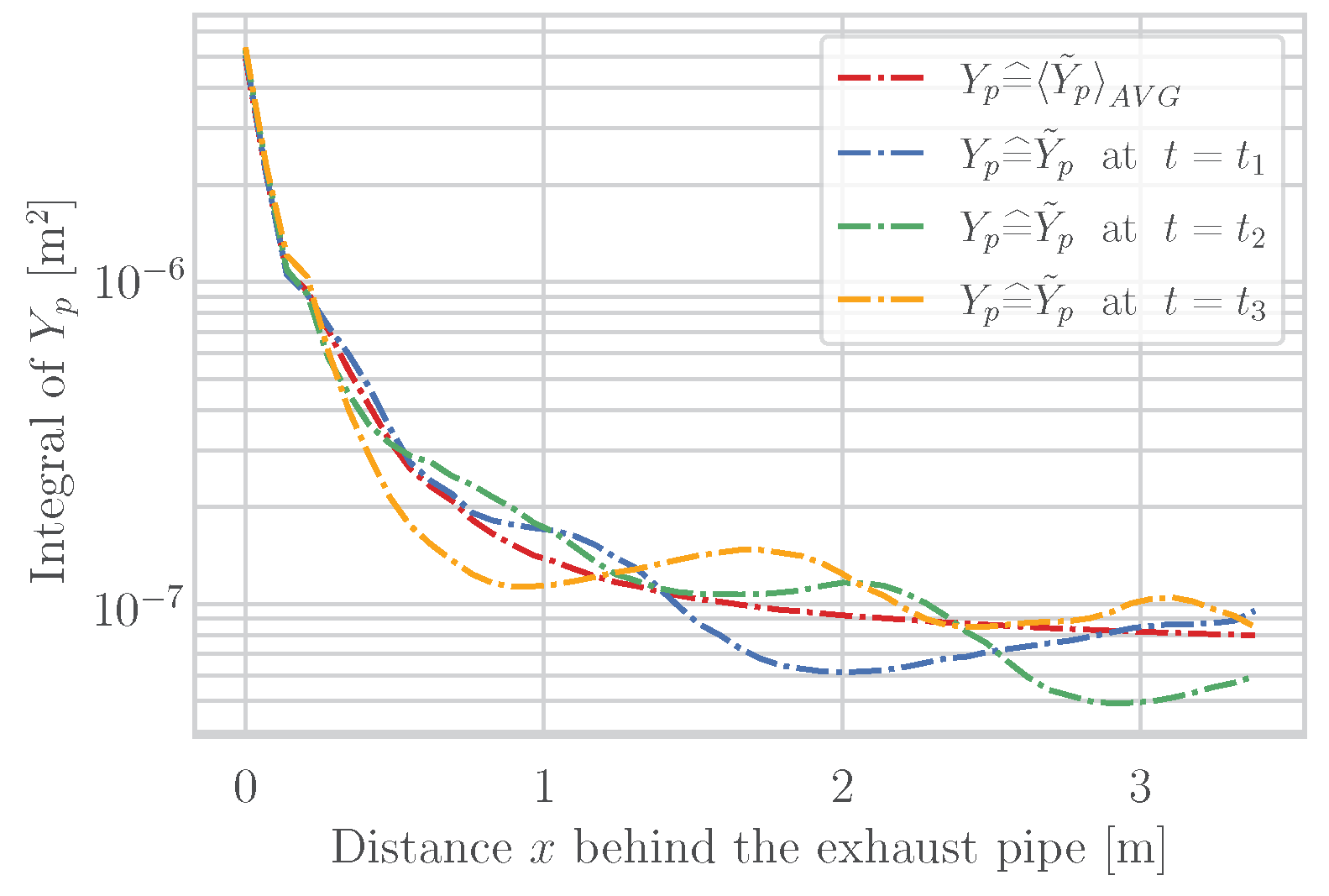
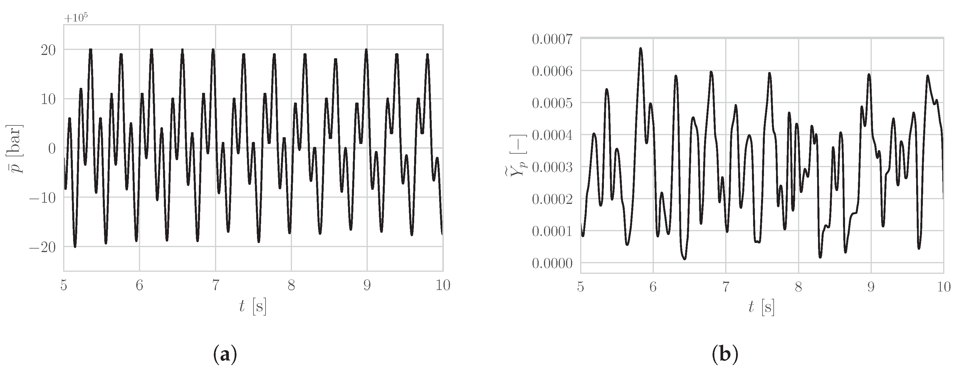
19) is what the plane-measurement instrument should theoretically measure. Since in RES the vehicle is moving while the measurement system is stationary at the roadside, 100 levels are taken in the simulation with a frequency of 200 Hz, over 0.5 s with increasing distance (according to the vehicle velocity) to the exhaust tailpipe. This way, the relative movement from the vehicle to the RES device is correctly represented. However, the URANS simulations performed show an unsteady flow behavior (see
Figure 4a). Since these vortices influence the transport of the exhaust gases, a different dispersion behavior of the exhaust plume can be observed at different starting times of the procedure just described (see
Figure 5 and related discussion).
Since it is unknown how a certain RES measurement correlates in time with the results of the simulation, a temporal averaging is introduced. The temporal information content of the simulations is lost, whereas now a general statement about the dispersion of the exhaust gases can be made independent of time. Due to the fact that long time-averaging describes a stationary state, the levels in the vehicle wake can just as well be taken at a point in time after averaging has taken place. Basis for the time-averaging is the quasi-periodic vortex shedding, as mentioned in
Section 2.3. Thus, pollutant mass fractions were averaged over a window of 20 periods after convergence was reached [
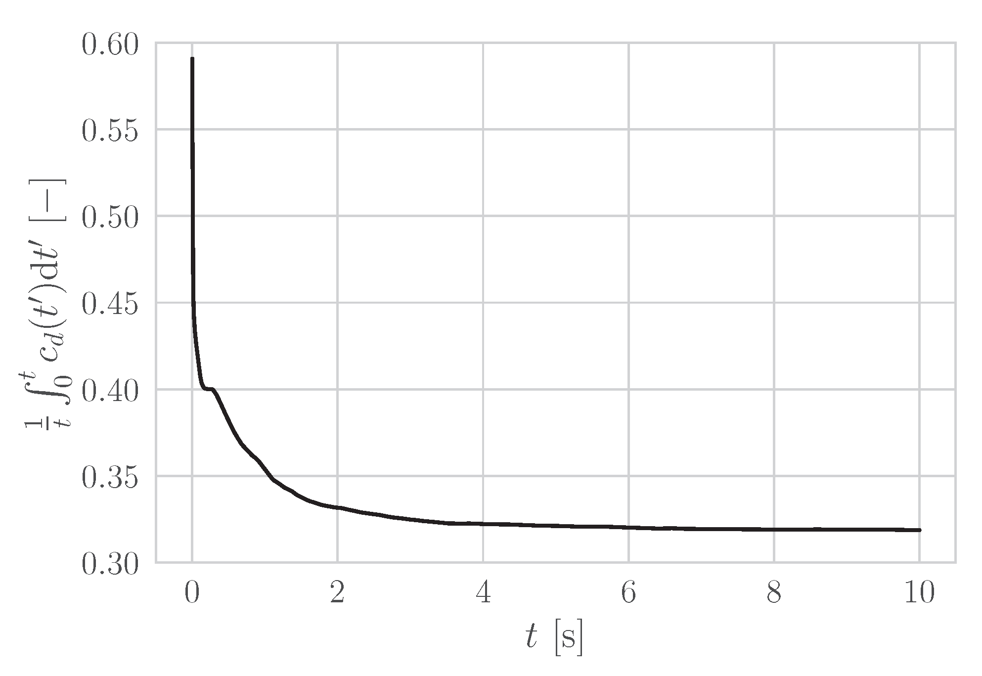
38]. Convergence can be observed when flow variables are oscillating around a mean and therefore, the respective residuals don’t change a lot anymore. As another criterion the running average of the drag coefficient
is computed and depicted in
Figure A1. As can be seen, convergence was achieved after approx. 5 s (or approx. 350 CPU hours), which is the case for the vast majority of simulations performed in this paper.
Figure A2a shows the pressure oscillations around the atmospheric pressure and illustrates well the quasi-periodic vortex shedding.
2.6. Exhaust Tailpipe Configurations
Typically, the exhaust tailpipes have two orientations, i.e., horizontal and downward oriented. Horizontal tailpipes are always at the rear of the vehicle at a position of . Downward oriented tailpipes are slightly shifted toward the rear wheels and placed at a typical position of . Thus, the investigated tailpipe positions are left horizontal (LH), central horizontal (CH), left/right horizontal (LRH) and left downward oriented (LD), central downward oriented (CD), left/right downward oriented (LRD). For all exhaust tailpipe configurations, the fraction of the exhaust plume upstream of the vehicle was not considered since a RES device would only measure downstream of the vehicle.
3. Results and Discussion
In order to study the influence of every parameter individually, the exhaust composition and mass flow has been kept the same throughout the parameter study. These values are taken from a chassis dynamometer measurement of a light duty vehicle at 50 km/h of a frequently sold compact-class gasoline vehicle. Thus, the exhaust gas species , , , , and yield a total mass fraction of 30.8%. The rest is split between with 0.005% and with 69.2%. The measured exhaust mass flow has been used to estimate the exhaust tailpipe velocity based on the tailpipe diameter, which is 5 m/s.
3.1. General Flow Characteristics
The flow around the vehicle is analyzed below at a constant vehicle velocity of 50 km/h. The Reynolds number based on the vehicle length for the investigated vehicle velocities of 30, 50 and 80 km/h is 2.48
, 4.13
and 6.61
, respectively, which thus characterizes a highly turbulent flow [
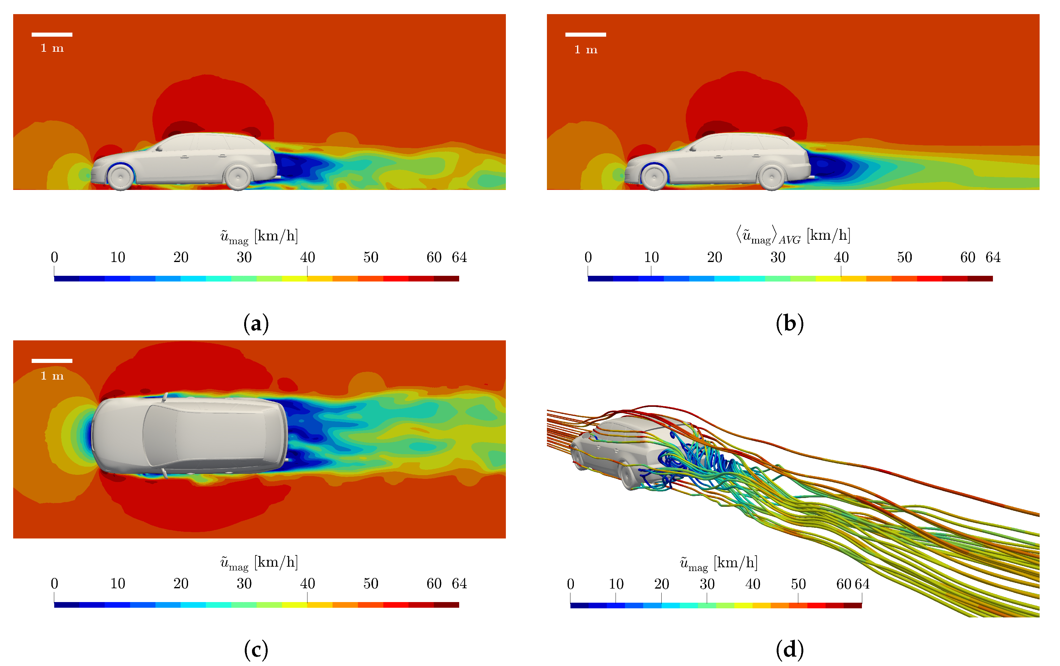
9]. In addition, continuous flow separation at the vehicle (e.g., in the rear and at the mirrors) results in a transient vehicle wake (see
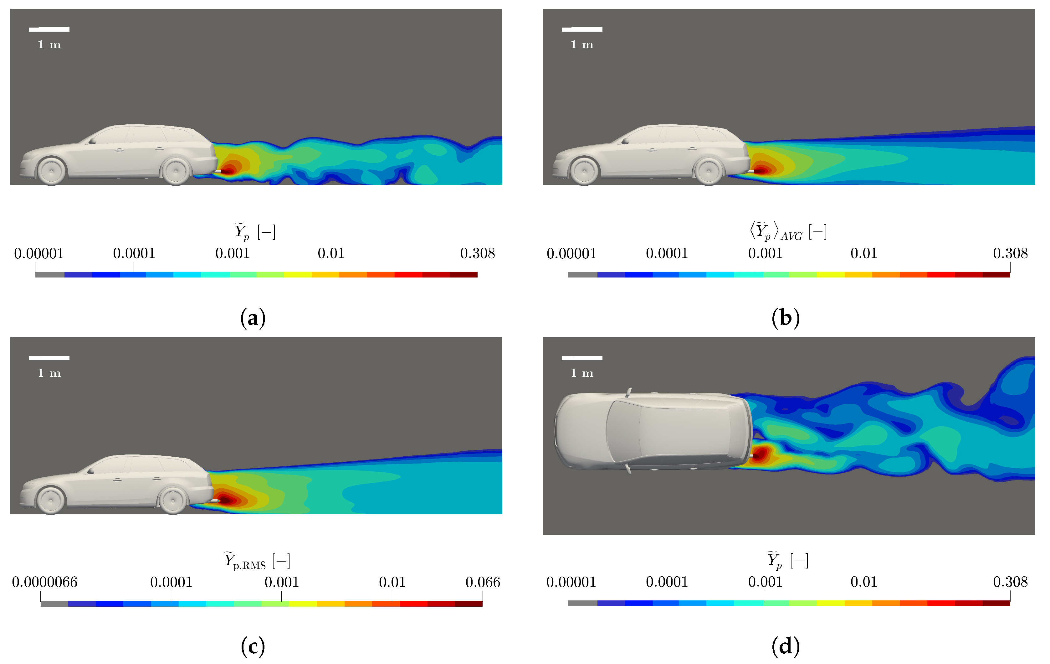
Figure 4d). The hot exhaust gas that enters the vehicle wake induces additional mass and heat transport. Since the mass flow of the exhaust gas is small compared to the mass flow of the ambient air (advection-driven flow), the heat transport is rather weak and the focus of further analysis lies on the transport of pollutants in the vehicle wake. In the following, the influence of the flow on pollutant dispersion is discussed.
The contour plots of the flow velocity in
Figure 4a,c clearly show the unsteady flow behavior in the vehicle wake, caused by continuous flow separation around the vehicle. The wake is thus geometrically determined by the height and width of the vehicle and equalizes with the undisturbed flow downstream. As discussed in
Section 2, URANS simulations have the advantage of resolving the unsteadiness of the flow. Thus, a temporally variant velocity field
was obtained as can be seen in
Figure 4a,c. In contrast,
Figure 4b shows a time-averaged velocity field. The unsteadiness is also evident in the evolution of the species concentration downstream of the vehicle as indicated in
Figure 5. Therefore, measuring at different time instants results in slightly different species concentrations. For the sake of comparability,
is used instead.
The recirculation zone behind the vehicle is confined to the near wake and is in the order of magnitude of a vehicle length. This region is of particular importance, since the convective flow velocity tends to zero toward the center of the recirculation zone and, in particular, turbulent velocity fluctuations increase compared to the free-stream region. Consequently, Reynolds stresses are increased in this region, which enhances turbulent mixing. Based on the modeling assumptions made, this is summarized by the eddy viscosity. As can be seen in
Figure 6, this is at a maximum of
in the wake of the vehicle. In contrast, the kinematic viscosity is 1.55
m
/s.
Consequently, the eddy viscosity in the near wake is nearly four orders of magnitude higher than the kinematic viscosity and dispersion is almost exclusively determined by turbulent mixing. Due to the strong turbulence described by , and , these parameters are multiple orders of magnitude higher than their molecular counterparts. Therefore, the influence of slightly different molecular diffusion coefficients for the different exhaust gases, such as CO and NO is negligible. Consequently, all species except O and N are grouped together as the exhaust gas or pollutant(s).
Figure 7a,d show the pollutant dispersion in the vehicle wake for a velocity of 50 km/h. The exhaust gases dilute very rapidly after they leave the tailpipe and enter the vehicle wake. To reach a hundredfold dilution of the exhaust tailpipe concentration, the exhaust plume has to be 0.83 m long (
x), is 0.81 m wide (
y), and 0.74 m high (
z), as can be seen in
Figure 7 and
Figure 8a (for a vehicle velocity of 50 km/h with the LH tailpipe). Other vehicle velocities and exhaust tailpipe positions investigated are discussed in
Section 3.2 and
Section 3.3.
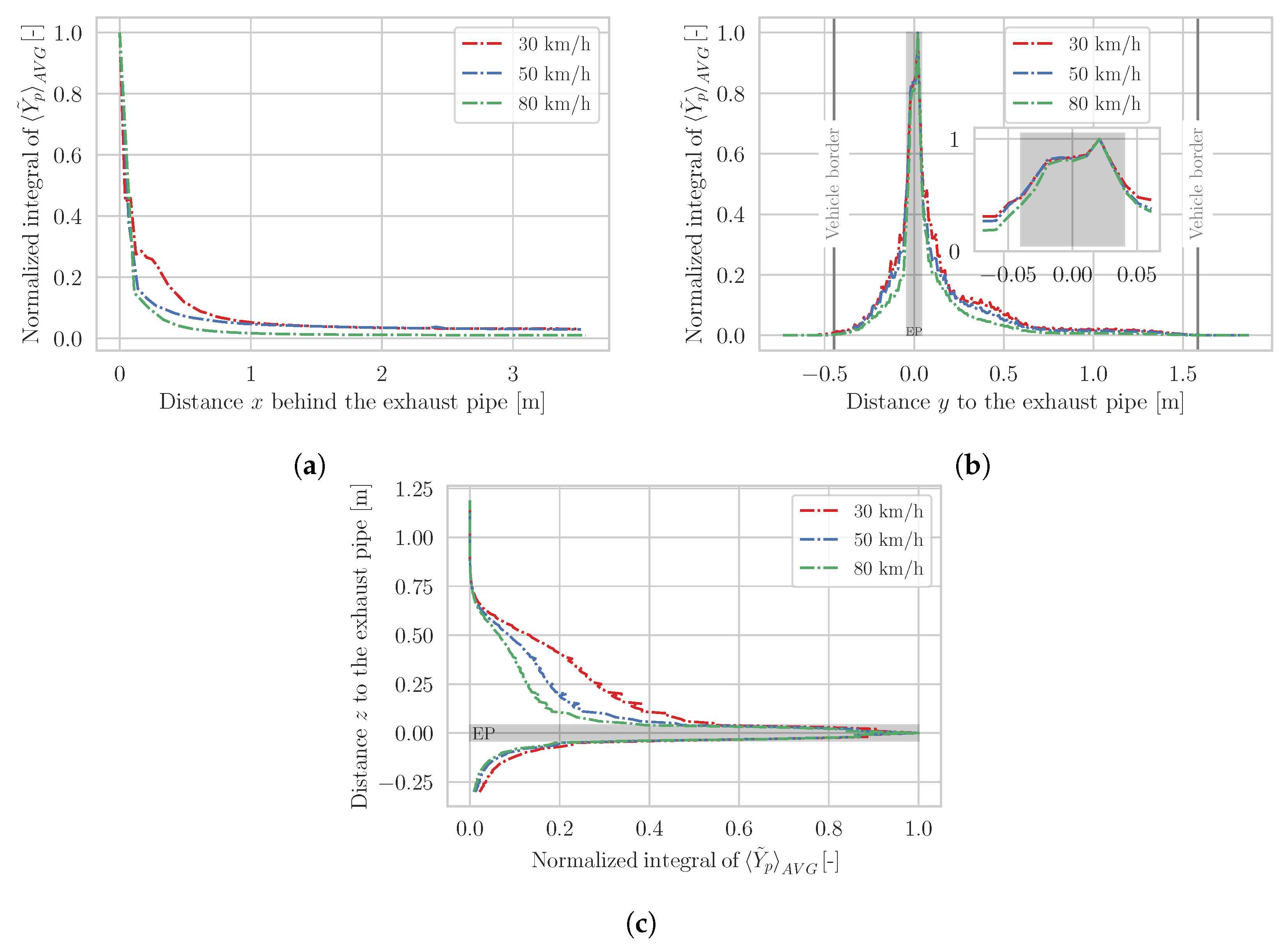
In
Figure 8b it can also be seen how the exhaust gas is distributed laterally with respect to the exhaust tailpipe (
y-direction). Again, large pollutant mass fraction gradients exist directly next to the exhaust tailpipe, so that 0.5 m to the side of the tailpipe a negligible amount of pollutant is present. Since this example involves an exhaust tailpipe on the left side of the vehicle, the dispersion curve is not symmetrical. Consequently, there is less pollutant 0.5 m to the left of the tailpipe than 0.5 m to the right of the tailpipe. At this point, it should be mentioned that this is a normalized sum of all pollutants on the
-planes.
The same evaluation can also be made for the
z-direction. The pollutant mass fraction is highest at the level of the exhaust tailpipe and decreases sharply both downward and upward. However, the exhaust gas is distributed more upward toward the rear window of the vehicle than downward toward the underbody of the vehicle. This is a consequence of the flow field as can also be seen in
Figure 4a,
Figure 6a and
Figure 7a and the recirculation zone, caused by detachments on the roof and underbody. The proximity of the exhaust tailpipe to the underbody means that some of the escaping exhaust gas is carried upward by the recirculation. Finally,
Figure 4a already indicates that above the exhaust tailpipe, the recirculation zone with lower velocities is prevailing while below the exhaust tailpipe convection due to the high mean flow velocity dominates.
3.2. Influence of Vehicle Velocity
Moreover, in
Figure 8, the same behavior can be observed for vehicle velocities of 30 km/h and 80 km/h as well. As the vehicle velocity increases, the concentration of pollutant in the
x-direction decreases more rapidly. Due to the increased mean flow velocity, turbulent mixing in the vehicle wake is intensified and the exhaust gas therefore mixes in the cross-flow directions (
-planes), where convective transport is equally low due to small mean flow velocities. In the
x-direction, convective transport dominates due to the high mean flow velocity and consequently transports the exhaust gas downstream at different rates for different vehicle velocities. For the velocities of interest, however, differences are small.
This trend is also evident for the other directions. Thus, with increasing vehicle velocity, the sum of pollutant concentrations decreases faster laterally from the exhaust tailpipe (
y-direction). In the closest proximity of the tailpipe, the influence of vehicle velocity is negligible (see insert of
Figure 8b). The same applies both toward the ground (
m) and toward the vehicle roof (
m), as can be seen in
Figure 8c.
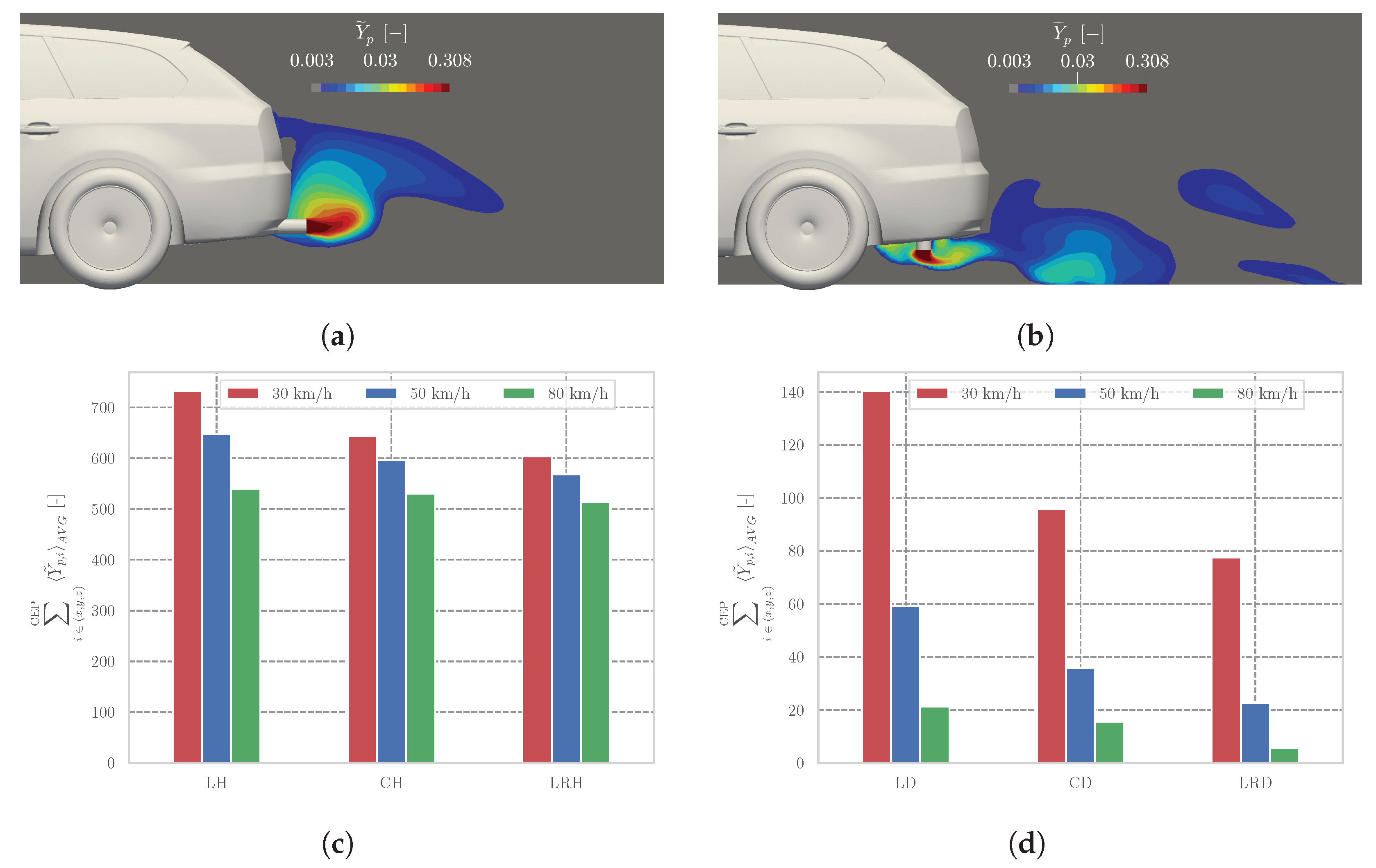
3.3. Influence of Exhaust Tailpipe Position
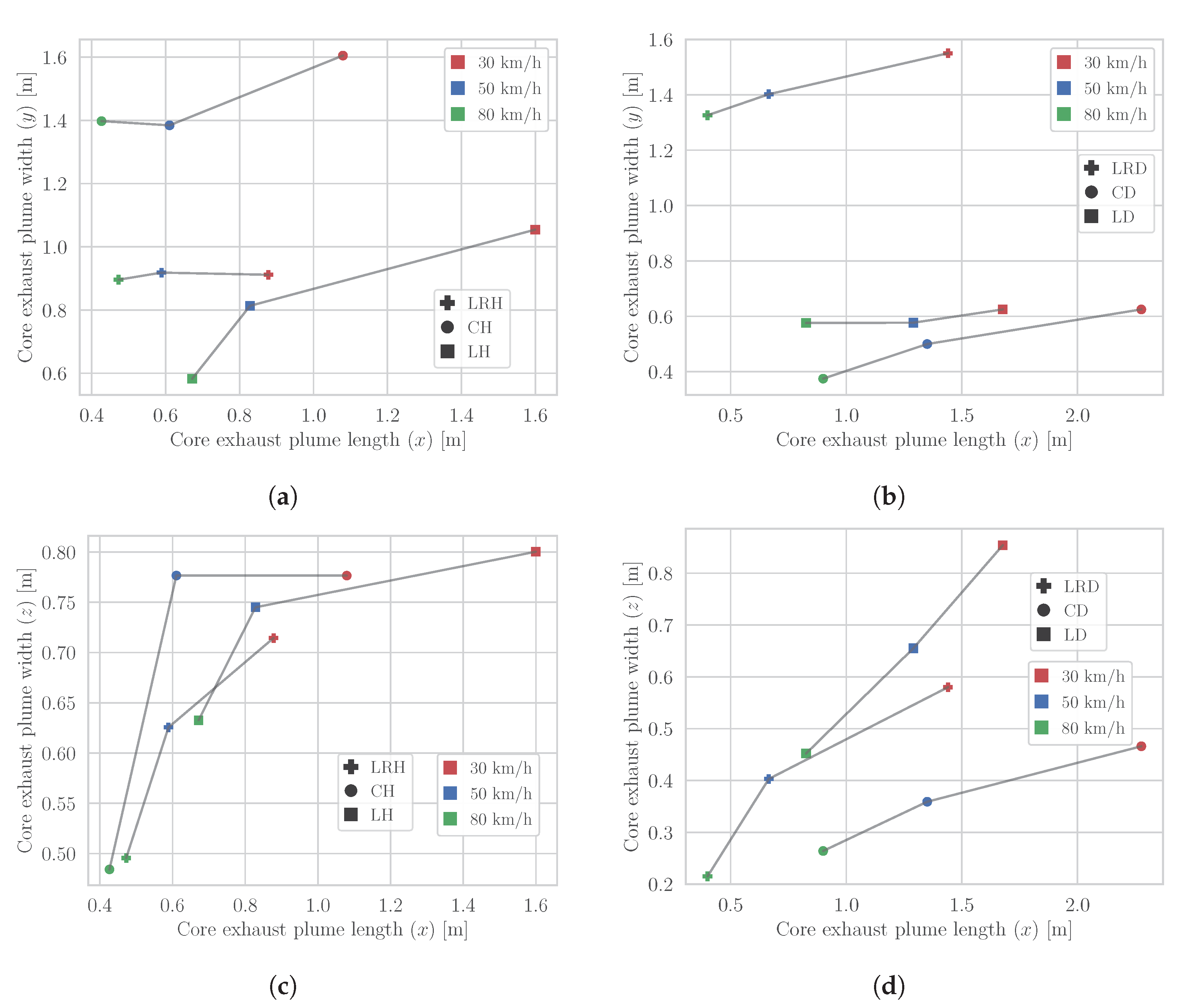
For the following evaluation, a core exhaust plume (CEP) is defined. This ranges from the exhaust tailpipe concentration of to , which corresponds to almost a hundredfold dilution. The size/scattering of the CEP is defined as the length (x), width (y) and height (z) of the resulting plume. However, one constraint is that the CEP has to be measurable and thus, only the CEP downstream the vehicle is considered in the following analysis.
According to the discussion in
Section 3.2, at higher vehicle velocities, the time-averaged exhaust plume becomes shorter (
x-direction) and narrower (
y,
z-directions). This is true for all horizontal (see
Figure 9a,c) and downward oriented exhaust tailpipes (see
Figure 9b,d). For horizontal tailpipes, the CEP shortens (
x-direction) significantly between velocities of 30 and 50 km/h. It also shortens between velocities of 50 and 80 km/h. but much less, despite a similar relative velocity increase (see
Figure 9a,c). The behavior reverses for the lateral coordinate
z, where the CEP narrows more significantly between 50 and 80 km/h than between 30 and 50 km/h. This effect is more pronounced for LH and CH tailpipe configurations (see
Figure 9c). In the
y-direction the CEP shows no clear tendency for different vehicle velocities as depicted in
Figure 9a.
The CH tailpipe is the one that produces the shortest but widest exhaust plume. The LRH tailpipe does not reflect a CEP twice as large as that of the left tailpipe. This is due to the fact that the exhaust gas mass flow is divided between the two tailpipe outlets and therefore smaller CEP’s are formed on the left and right compared to a LH tailpipe. In addition, the CEP of an LRH tailpipe shows almost constant width (y-direction) as vehicle velocity increases.
Downward oriented tailpipes result in greater CEP dimensions as the horizontal counterparts (compare
Figure 9a,b and
Figure 9c,d). Here, the exhaust gas is not ejected into the wake region (such as exists downstream the vehicle), but below the vehicle underbody, where convective transport dominates due to a higher mean flow velocity compared to that in the wake region. Furthermore, the exhaust gas is ejected perpendicular to the main flow direction as opposed to the horizontal tailpipes (compare
Figure 10a to
Figure 10b). As a result, the CEP of downward oriented tailpipes is located more toward the road and is transported further downstream (
x-direction).
The CD tailpipe is the one that produces the longest (
x-direction) but narrowest (
y,
z-directions) CEP (see
Figure 9b). In contrast, the LRD tailpipe results in the shortest (
x-direction) but widest (
y-direction) CEP. The LD tailpipe has a wide CEP (
z-direction) and an insensitive size in
y-direction with regard to changes in the velocity. Overall, for all downward oriented tailpipes the change of the CEP size when velocity increases appears to be more linear and more pronounced than it is the case for horizontal tailpipes. This is especially true for the
z-direction, where only a small change in the size (
z-direction) can be observed for horizontal tailpipes (compare
Figure 9c and
Figure 9d).
In addition to the size/scattering of the CEP, the amount of exhaust gas in this CEP can also be compared for the different tailpipe positions and vehicle velocities. For this purpose, the sum of the mass fractions of all pollutants within the measurable CEP is calculated. In
Figure 10c,d it can be seen that for each tailpipe configuration, the size of the CEP decreases with an increase in velocity. This is the case for both the horizontal and the downward oriented tailpipes. Specifically, for the downward oriented tailpipes the difference between 30 km/h and 50 km/h is greater than between 50 km/h and 80 km/h.
It also is particularly interesting to note that not only for a specific exhaust tailpipe configuration the amount of pollutants in the CEP decreases with velocity, but also for all different velocities the amount of pollutants in the CEP depends on the exhaust tailpipe position. Thus, for both horizontal and downward oriented tailpipes the amount of pollutants in the CEP is greatest for tailpipes on the left (LH and LD). The amount of pollutant is then less for that in the center of the vehicle (CH and CD) and smallest for the two-sided (left and right) tailpipe configuration (LRH and LRD). Since only the CEP downstream the vehicle is considered in this analysis, to determine the concentration available for a RES measurement the amount of pollutant in this CEP is smaller for downward oriented tailpipes. As shown in
Figure 10b, the CEP with higher pollutant concentrations is located upstream of the rear of the vehicle and thus left out for the estimation of the numbers presented in
Figure 10d.
Consequently, this has implications for a RES measurement. For downward oriented tailpipes, it is more unlikely that the measurement will be successful, since the CEP with higher pollutant concentrations is underneath the vehicle and can thus not be detected by RES devices. However, there are differences for the aforementioned tailpipe configurations. The exhaust gas mass flow as well as the pollutant concentration at the outlet of each tailpipe is identical, so that in the optimal case that measurement should achieve the same pollutant concentration for all tailpipe configurations. Since the pollutant concentration is proportional to the absorption of the light/laser barrier and the measured absorption is greater the more exhaust gas passes the light/laser barrier, vehicles with LH tailpipes are the most sensitive, whereas LRD tailpipes are the least sensitive. As explained earlier, however, this phenomenon becomes more and more negligible with increasing velocity.
3.4. Influence of Crosswind
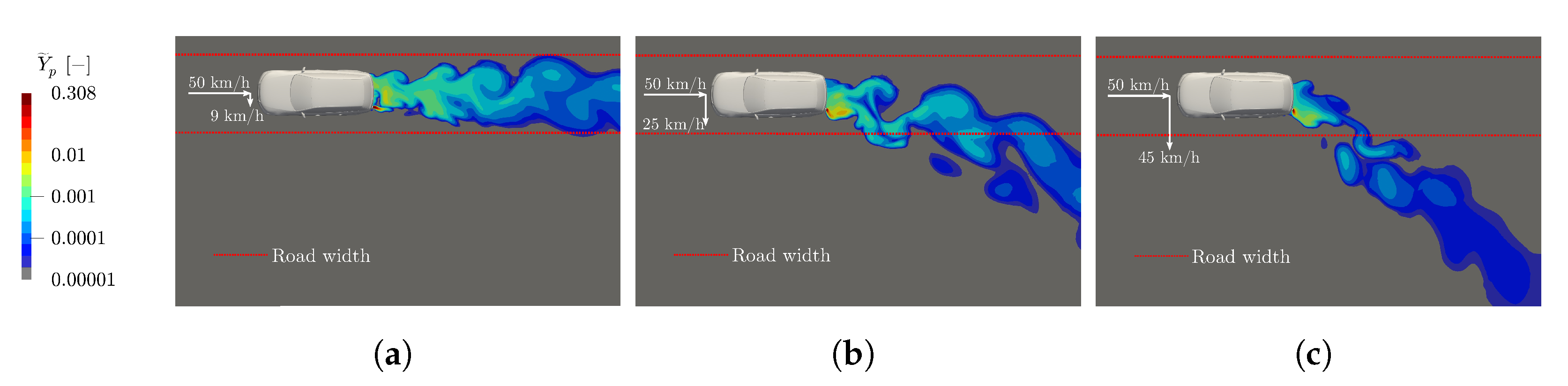
Under the influence of wind, the exhaust plume is deflected into the corresponding wind direction. The cases considered here are direct crosswinds (90°) from the right. In the course of the parameter study, other wind directions (30° and 60°) from the right and from the left were also investigated.
Figure 11 shows the exhaust plume under the influence of three different wind strengths. These are a light breeze (2 Bft or 9 km/h wind velocity), medium breeze (4 Bft or 25 km/h wind velocity) and a strong breeze (6 Bft or 45 km/h wind velocity). Higher wind velocities in urban as well as rural areas are rather uncommon and therefore not considered further [
39].
With increasing wind velocity, the exhaust plume is deflected stronger. In addition, the oscillations in the exhaust plume strongly increase even with a light breeze, as can be seen from the contours of the exhaust plume. This becomes more pronounced at higher wind velocities, where vortices increasingly detach in the wind direction. For RES this means that the exhaust plumes deflected by wind from vehicles on another lane can interact with one’s own exhaust plume and falsify a measurement. However, the deflected part of the exhaust plume already is strongly diluted and the CEP remains close behind the vehicle, as can be seen in
Figure 11.
The deflection of the plume influences the RES result, as RES devices use all samples from each measurement for deriving the final result (as further discussed in
Section 3.5). Thus, a larger distance between transmitter and reflector (in case of a line-measurement device), often limited by the road width, allows to capture more of the plume in the case of crosswind deflection. Therefore, for the following investigations we added as a parameter the distance between transmitter and reflector, i.e., the road width.
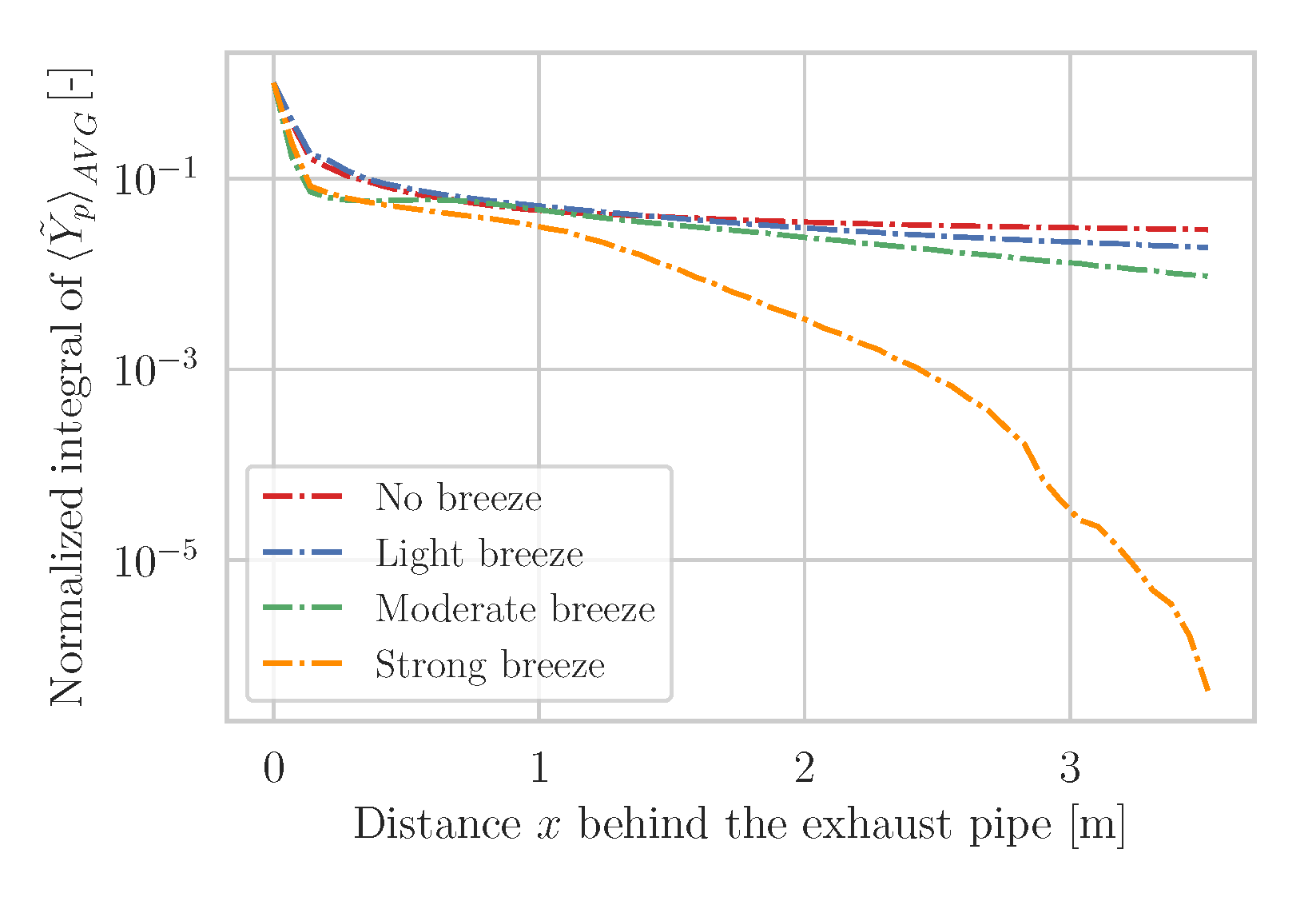
All investigated wind directions and angles result in similar behavior of the plume.
Figure 12 illustrates this behavior: Near the exhaust tailpipe the wind has weak, if any, influence on the exhaust plume. However, with increasing distance from the tailpipe and with increasing wind the amount of pollutant decreases, which in the optimum case can be detected by RES devices at a fixed road width of 3 m.
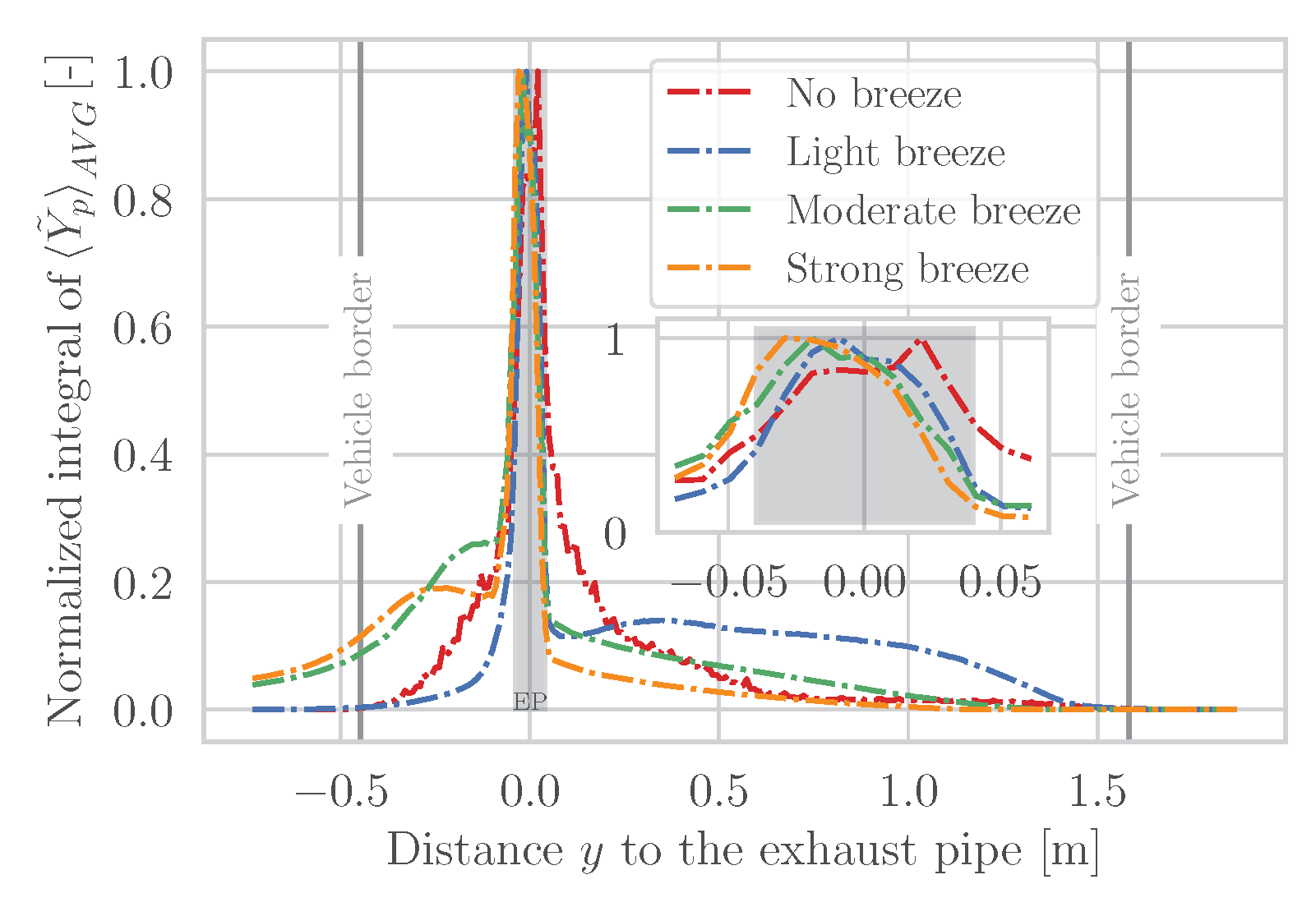
Figure 13 compares the dilution of the exhaust plume in the lateral coordinate
y. Since the exhaust gas still comes from the same exhaust tailpipe position, the pollutant concentration peaks still are within the tailpipe diameter for all cases. Nevertheless, the wind makes itself slightly noticeable, since with increasing wind velocity (from right to left), the pollutant peak moves to the left.
As already qualitatively explained on the basis of
Figure 13, it can be seen that, due to the wind, a part of the exhaust plume is shifted further to the left and the sum of the pollutant concentrations in the
-planes thus does not yet tend toward zero on the left side of the vehicle. In the case of a light breeze, however, this behavior is not yet present. Here, the large coherent vortices still hold together and have not yet separated in the
y-direction. The vast majority of the exhaust plume therefore remains behind the vehicle and even shifts a little to the right relative to its own maximum where a plateau is prevailing toward the right vehicle border (
m).
3.5. Different RES Devices
The simulations result in concentration fields of the pollutants in the vehicle wake which are measured by the RES devices. As already discussed in
Section 2.5, the existing RES devices have different characteristics which lead to different parts of the captured and analyzed wake contributing to the final measurement result. In this Section, we investigate the differences in the captured concentration field by the RES based on different optical setups (line- and plane-measurement) and different sampling frequencies. In addition, we investigate the influence of different distances between the transmitter and the reflector of the line-measurement device as can be given by different road widths.
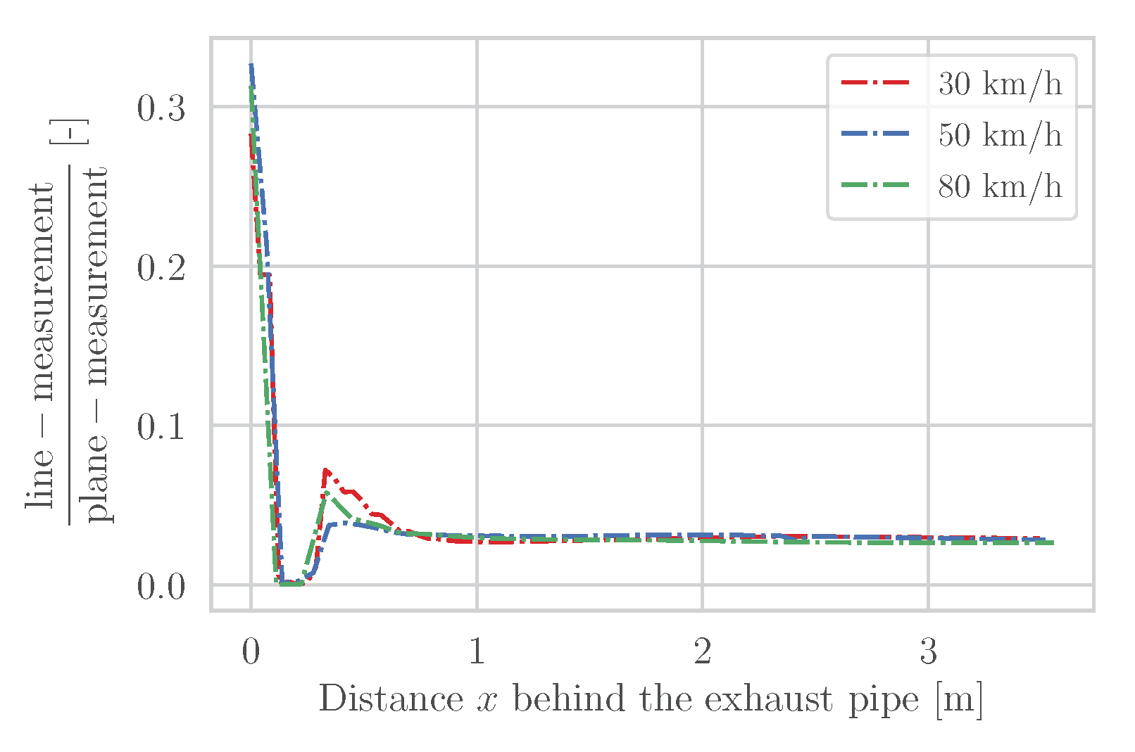
Figure 14 displays the ratio of the pollutant concentrations in the wake that can be measured by a line-measurement instrument to the pollutant concentrations that can be measured by a plane-measurement instrument. It is assumed that the line-measurement instrument is positioned exactly on the height of the tailpipe. As expected, the plane-measurement device can capture significantly more of the pollutants, that is 70% more in the direct vehicle vicinity and approximately 95% more in larger distances downstream the vehicle. This is due to the fact that the exhaust plume travels above and below the light beam of the line-measurement instrument and thus only a fraction is captured. However, other vehicles might have lower or higher tailpipe locations and the absorption level would be even lower.
Figure 14 additionally illustrates how the exhaust plume in the near wake always moves in and out of the light beam of a line-measurement instrument, since the ratio just starts becoming constant after 1 m downstream the tailpipe.
From this it can be concluded that theoretically the plane-measurement instrument has a clear advantage in the detection of exhaust gas in the vehicle wake. Since absolute sensitivities are not known for either technology, it is difficult to say at what point the absorption of a given species is too small to produce a valid measurement (concentration ratio). However, it is likely that individual measurement points of an entire line-measurement will hardly absorb anything, and therefore invalid measurements may occur more often, since no concentration ratio can be determined according to the principle described in
Section 2.5. Moreover,
Figure 8c illustrates that positioning the light beam not at exhaust tailpipe height has enormous effects on the detection of pollutants. However, a slightly higher position of the light beam is advantageous as opposed to a lower position, since pollutants are rather transported upward.
As already mentioned in
Section 2.5, the plane- and line-measurement instruments sample the exhaust plume with different frequencies. Therefore, depending on the frequency, more or less points are sampled over a certain duration. In the case of the line-measurement instrument, originally 50 measurement points were used at 100 Hz over 0.5 s. In the end, the concentration ratios are determined via a least square fit [
33]. This in turn means that a correct concentration ratio not only depends on the measurements near the exhaust tailpipe, but also on those further downstream of the vehicle.
At a frequency of 100 Hz and a measurement duration of 0.5 s, a vehicle velocity of 50 km/h results in a distance of 6.95 m over which 50 absorptions are measured in the vehicle wake, if the measurements directly start at the exhaust tailpipe. Our simulations have shown that it does not make much difference which frequency is used for the measurements, except for the first 20 cm after the exhaust tailpipe. Due to the low sampling rate of 100 Hz, the next measurement point is 13.89 cm away from the exhaust tailpipe (for a velocity of 50 km/h) and the dilution of the exhaust plume up to that point already is about 80% in terms of the maximum cut plane integral of pollutant mass fraction in the -plane at tailpipe exit ().
This underlines that the line-measurement instrument is rather unsuitable for higher velocities (>80 km/h), since then the first measurement point is more than 22.22 cm behind the vehicle.
Figure 8a shows that in this range a large part of the dispersion already has taken place. Consequently, possible measurement problems result from the fact that the line-measurement instrument measures too slowly and thus includes a high proportion of too diluted measurement points (below the sensitivity limit of the measurement instrument) into the calculations.
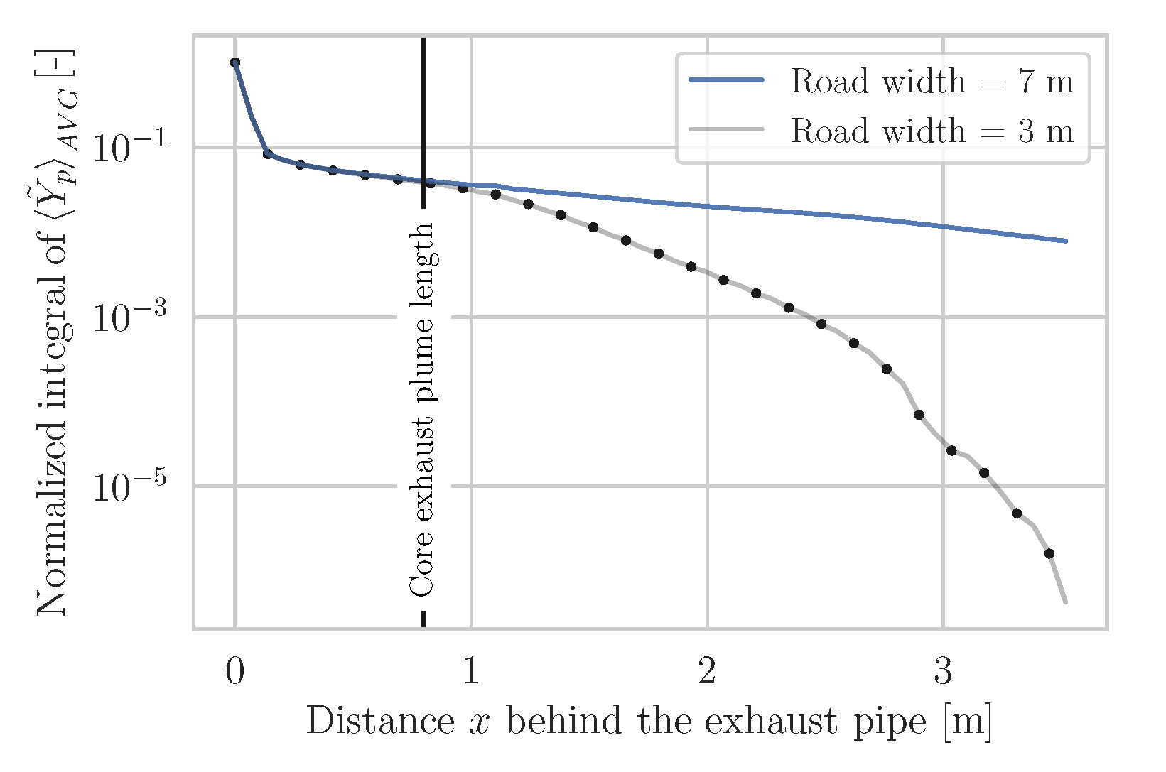
In case of crosswind, a low frequency measurement system has further difficulties. For the case of wind blowing from the side (90°) at 45 km/h, the CEP remains behind the vehicle. Further away from the vehicle, however, the exhaust plume is deflected and is no longer within the measurement range. This wind velocity corresponds to a strong breeze of 6 Beaufort. In addition,
Figure 15 shows the dispersion curve of this wind simulation for different road widths. In the case of a road width of 7 m (blue), a part of the exhaust plume still is recorded, which is not captured for a narrower road of 3 m (gray). Although the different frequency measurements agree there, measurement points that far downstream are not necessary for higher frequencies. In the case of 1000 Hz and the assumption that 50 measurement points are sufficient, measurements only are necessary up to 0.695 m (or equivalent for 0.05 s) downstream of the vehicle. As
Figure 15 clearly shows, up to this distance behind the vehicle no significant deflection of the exhaust plume has occurred. Thus, at this frequency, with a road and measurement width of 3 m and the considered limiting case of 45 km/h wind velocity, almost 100% of the exhaust gas can be detected. Of course this only applies to the case where the measurements are based on planes and not lines/beams. For even higher frequencies such as 10,000 Hz, the wind poses even fewer problems, as long as 50 or similar measurement points are sufficient to reconstruct the concentration ratio. Measurements in the cut planes are taken at a frequency in this order of magnitude.
3.6. Influence of a Vehicle Upstream
In order to evaluate the influence of the exhaust plume from an upstream vehicle, a computational domain similar to the one from
Section 2.2 was created. Here, two identical vehicles were placed 10 m apart (in the direction of motion) in one case and 25 m apart in the other. The distance of 10 m is considered too close for a vehicle velocity of 50 km/h (according to road traffic law it should be at least 25 m). The two vehicles emit the same amount of exhaust gas as summarized in
Section 3.
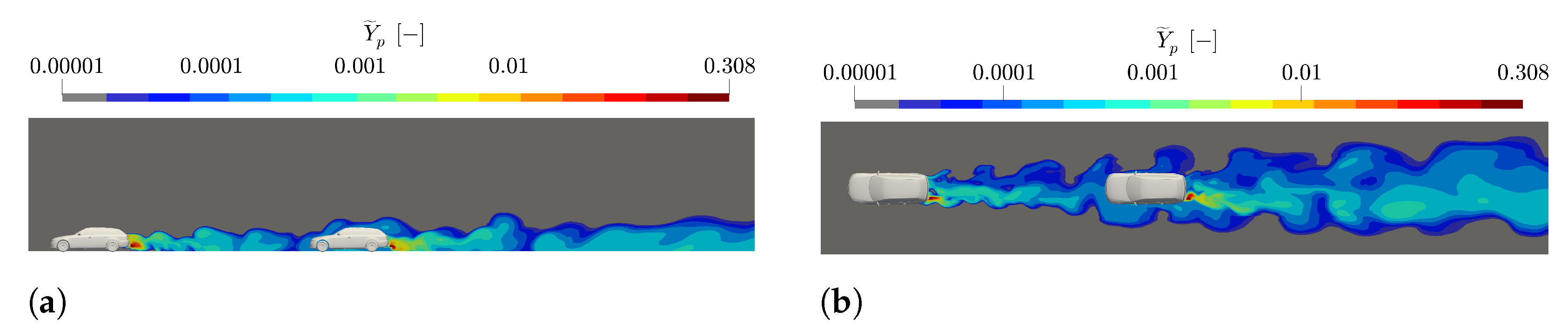
In
Figure 16, the influence of the vehicle upstream is clearly visible. The exhaust plume hits the second vehicle and then is deflected around the vehicle. Since the exhaust tailpipe is located on the left side of the vehicle (standard case, see
Section 3.3), the deflection of the exhaust plume appears to be slightly more to the left. Also seen is that the CEP from the second vehicle is affected due to the complex flow structures induced from the first one. To illustrate the interference of multiple exhaust plumes and its influence on the measurements,
Figure 17 shows the pollutant dispersion in the direction of motion (
x-direction).
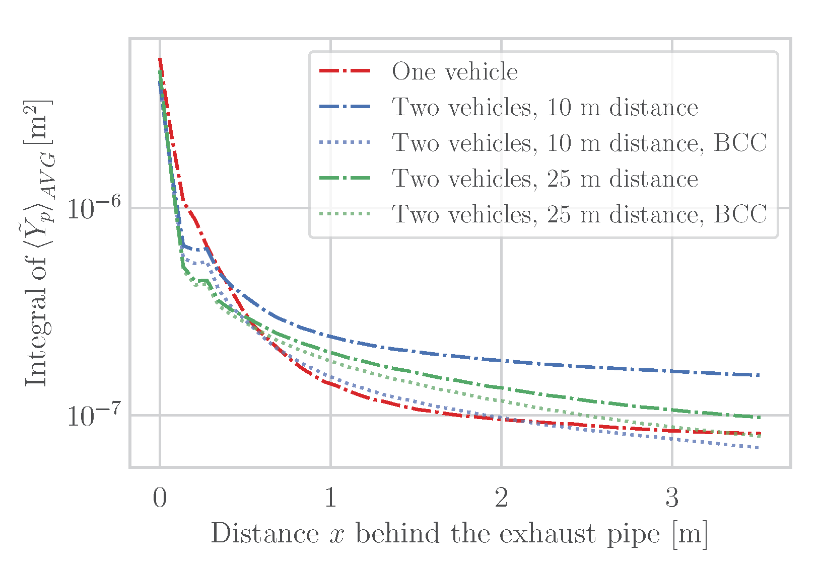
Contrary to the intuitive expectation, no higher pollutant concentration is detected in the near-wake (
m) of the second vehicle. Therefore, the initially larger drop in the pollutant concentration of the second vehicle (both 10 m and 25 m downstream of the first vehicle) is due to the stronger mixing upstream of the second vehicle (compared to the first vehicle). Due to continuous vortex shedding of the first vehicle, the flow downstream of the second vehicle is more chaotic and turbulent diffusion is larger than downstream of the first vehicle. In addition, again a limited road width was selected (3 m), such that the part of the exhaust plume which spread out of these limits is not taken into account.
Figure 16 also shows that the CEP of the second vehicle is more compact (with respect to the first vehicle), especially in the
y- and
z-directions. Therefore, a larger part is transported downstream (
m). This correlates well with
Figure 17.
However, it should be mentioned that RES devices consider background concentrations (sampled pollutant concentrations upstream the measured vehicle), see
Section 2.5. This is considered in
Figure 17. Taking background concentration correction (BCC) into account, we can conclude that the influence of an upstream vehicle on the measurements is negligible. As the distance between vehicles increases the background pollutant concentration is lower and the effect of the background concentration correction becomes more negligible.
In summary, the interference of pollutant concentrations from multiple longitudinal exhaust plumes has a smaller effect on accuracy than the increased turbulent intensity induced by the vehicle ahead, which alters the general evolution and dispersion of the second exhaust plume. Consequently turbulent mixing as well as convective transport in the exhaust plume of the second vehicle are influenced by the wake of the one ahead. Regarding the distance between the vehicles, no major sensitivity can be observed, if the background concentration properly gets adjusted.

 ,
, 


