Article

IoT-Based Bi-Cluster Forecasting Using Automated ML-Model Optimization for COVID-19

1
Department of Electrical Engineering, College of Engineering, Qatar University, Doha 2713, Qatar
2
Dipartimento di Ingegneria delI’Informazione, Brescia University, 25121 Brescia, Italy
3
Department of Computer Engineering and Computational Sciences, Canadian University Dubai, Dubai 117781, United Arab Emirates
*
Author to whom correspondence should be addressed.
Atmosphere 2023, 14(3), 534; https://doi.org/10.3390/atmos14030534
Submission received: 27 December 2022 / Revised: 16 February 2023 / Accepted: 27 February 2023 / Published: 10 March 2023
(This article belongs to the Special Issue Indoor Air Pollutants and Public Health)

Abstract

:
The current COVID-19 pandemic has raised huge concerns about outdoor air quality due to the expected lung deterioration. These concerns include the challenges associated with an increase of harmful gases like carbon dioxide, the iterative/repetitive inhalation due to mask usage, and harsh environmental temperatures. Even in the presence of air quality sensing devices, these challenges can hinder the prevention and treatment of respiratory diseases, epidemics, and pandemics in severe cases. In this research, a dual time series with a bi-cluster sensor data-stream-based novel optimized regression algorithm was proposed with optimization predictors and responses that use an automated iterative optimization of the model based on the similarity coefficient index. The algorithm was implemented over SeReNoV2 sensor nodes data, i.e., a multi-variate dual time-series sensor, of the environmental and US Environmental Protection Agency standard, which measures variables for the air quality index using air quality sensors with geospatial profiling. The SeReNoV2 systems were placed at four locations that were 3 km apart to monitor the air quality and their data was collected at Ubidots IoT platform over GSM. The results have shown that the proposed technique achieved a root mean square error (RMSE) of 1.0042 with a training time of 469.28 s for the control and an RMSE of 1.646 in a training time of 28.53 s when optimized. The estimated R-Squared error was 0.03, with the Mean-Square Error for temperature being 1.0084 °C, and 293.98 ppm for CO2. Furthermore, the Mean-Absolute Error (MAE) for temperature was 0.66226 °C and 10.252 ppm for the correlated-CO2 at a predicted speed of ~5100 observations/s. In the sample cluster for temperature, 45,000 observations/s for CO2 was achieved due to the iterative optimization of the training time (469.28 s). The correlated temperature and a time of 28.53 s for CO2 were very promising in forecasting COVID-19 countermeasures before time.

1. Introduction

According to the WHO and US Environmental Protection Agency (EPA) guidelines, the future of air quality and climatic conditions are a signature of life security for healthy respiration. The quality of respiration and its associated life processes are directly related to air quality, specifically in regard to oxygen (O2) and carbon dioxide (CO2) in a particular geo-location at a tolerable temperature (WHO, 2021) [1]. The National Ambient Air Quality Standards (NAAQS) report that the gradual deterioration in urban air quality is ambient each year due to the increasing population, chemical emissions from machinery, and depreciation in green ecology [2]. Several studies have concluded that a poor air quality index (AQI) refers to a higher concentration of CO2 in the atmosphere and that temperature extremities are more likely to be disastrous and fatal when it is inhaled/exhaled. Therefore, its real-time monitoring is key to public safety [3]. Mandated measurement methods, like geo-spatially sensed outdoor gases, are a critical decision source in forecasting the COVID-19 threat intensity at lower temperatures and higher CO2 concentrations [4]. Flu-based pandemics and COVID-19 are becoming an increasing problem worldwide and so require a more widespread research approach.
Globally, CO2 sensing time-series analysis and forecasting are the most widely capitalized approach in respiratory research i.e., an ensemble time-series model with machine learning approaches as the projection benchmark has shown that China’s carbon peak will be achieved by 2021–2026 with  >80% probability [5] by using the logged dataset with a gap in real-time CO2 sensing at regional temperatures. The Long Short-Term Memory (LSTM) networks, DeepLMS, resulted in an average testing Root Mean Square Error (RMSE) < 0.009, and an average correlation coefficient between ground truth and predicted values r ≥ 0.97 (p < 0.05) when tested on logged data from one database pre-COVID-19 and two during COVID-19 pandemic years [6]. This study [6] had challenges with data interpretation and collective forecasting from multiple real-time CO2 and temperature sensing units due to data structuring challenges. The first step has been structuring the dual-series sensor data into a decomposed time series, as mentioned in the reviews as either additive or multiplicative by valued research [7,8,9].
The second challenge was to sort the time-series in preparation for the next stage, called the time-series trend assessment using Theil-Sen’s Slope (TSS), Mann-Kendall (MK), Modified Mann-Kendall (MMK), and Kendall Rank Correlation (KRC) tests, which need the incorporation of improved trending for seasonality tests [8,9]. Several studies used the above-mentioned tests effectively for the logged data but they had challenges with real-time sensor data. The real-time processing, time-series decomposition methods (REG and GAM based on OLS; FFT, FFT, AVG, LOESS, and LHM based on Backfitting [10]) had challenges with the stationarity assessment. Various time-series hypothesis tests, the Durbin-Watson test (DWT), Box-Pierce (BPT), Ljung-Box tests (LBT), Breusch-Godfrey test (BGT), Jarque-Bera test (JBT), and Augmented Dickey-Fuller test (ADFT) were used for stationarity and seasonality assessment and are useful for the auto-regressive moving average (ARIMA); however, the advanced Seasonal autoregressive integrated moving average model (SARIMA) [11] needed a clustered approach for real-time forecasting of multi-variate sensor data. The statistical techniques and machine learning approaches mentioned above were found to have the sensors’ dependent and wireless sensor network-based anomalies’ dependent results.
The third major challenge was the absence of an optimized and adaptive real-time forecasting approach for the networked CO2 and temperature measurement sensor nodes. For this, many air quality sensing systems were studied. The top sensing systems AirNut, PA-I and PA-II, Egg, PATS+, and S-500, CairClip, Portable ASLUNG, AirSensEUR, Met One, AQY v0.5, Vaisala AQT410, 2B Tech, and AQMesh V3.0 systems had measurement capabilities for specific pollutants and gases [12]. This was impacted by real-time health monitoring systems [13] and the infrastructure and architectures of specialized platforms [14]. FIS SP-61, O3-3E1F, AirSensEUR v.2, S-500, and AirSensEUR used a built-in AlphaSense OX-A431 limited to O3 [15]. Likewise, the PMS1003 and PMS3003 by Plantower; DC1100 PRO and DC1700 by Dylos; and OPC-N2 by AlphaSense only had sensing support for particulate matter (PM) and so, from a multi-agent perspective, had challenges in the clinical biomarker space of COVID-19 using feature selection and prognosis classification for the time-series forecasting problem [16]. The networked sensing errors found in the previously mentioned works using CO-3E300 by City Technology; CO-B4 by Alphasense, MICS-4515 by SGX Sensortech, and Smart Citizen Kit by Acrobotic, and the RAMP had wireless sensor network errors that can be corrected by the multi-objective prediction monitoring algorithm [17,18,19]. All the above-mentioned research was suited for a fixed network of sensing systems but had to face the challenge of threshold updates that gave errors in forecasting spatially placed sensing node clusters [20].
In clustered sensing for CO2 and temperature, there was a pressing need for a concurrent forecasting chain in addition to a dimensionality reduction using matrix factorization (MF) [21] for the air quality nodes, with parametric ML model deployment support on embedded systems like SeReNoV2 [22]. Considering the recent studies conducted at the European Commission, Joint Research Centre (JRC) [23] on the impact of masks on CO2 concentration zones in the breathing zones, it was concluded that the increase in CO2 was due to breathing exhaled air temperature as well [24].
The existing O-AQNs, Urban AirQ, Smart Citizen Kit, Air SensUR 4.0, SeReNo V1, and AirQ Mesh needed improvement for the AQI-dependent principal component approach [25] in the scope of automated optimization of forecasting. The multi-time series-based forecasting required a novel melioration in linear regression and a tree-based time-series learning, regression, and forecasting tree to be an innovative step in the SeReNoV2 AQM systems.
The recent environmental data forecasting works (2022, 2023) were also reviewed. The hybrid additive regression and data-driven models [26,27] were monthly based and for arid environmental conditions had the gap of annual forecasting using real-time sensing systems [12,13,14,15,16,17,18,19]. The hybrid metaheuristic algorithms-based estimation of reference evapotranspiration [28] had challenges in real-time IoT-based sensing. The hybrid machine learning-pedotransfer Function (ML-PTF) based on a novel Genetic Algorithm (GA) for the prediction of the spatial pattern of saturated hydraulic conductivity [29] was more concentrated in the water patterns and needed improvements in real-time IoT-based environmental systems integrated data. The recent work in Runoff-Rainfall (R-R) [30] was a better contestant for several data-driven models, namely, multiple linear regression (MLR), multiple adaptive regression splines (MARS), support vector machine (SVM), and random forest (RF), but needs improvement in the IoT-based environmental and health integrated forecasting domain. Furthermore, very recent work in forecasting conducted a feasibility study to examine the feasibility and effectiveness of the Random Subspace (RSS) model and its hybridization with the M5 Pruning tree (M5P), Random Forest (RF), and Random Tree (RT). It was based on the data from the Standardized Precipitation Index (SPI) [31] case study in Jaisalmer, India and needed improvements in real-time IoT-based environmental sensing. A noticeable work was a study of the evaluation of the adaptive neuro-fuzzy inference system (ANFIS)-, artificial neural network (ANN)-, and wavelet-based artificial neural system (WANN)-based models [32] that estimated the discharge by using 12 years of daily data (2007–2018) but needed improvement in the IoT-based real-time sensing data and health integration application domain. The study of two different agro-climatic zones, that employed the data intelligence model and meta-heuristic algorithms-based pan evaporation modelling using the data from a case study from Northern India [33], needed an investigation into the same methods of the real-time IoT-based environmental data. The summary of enhancements is presented in Table 1.
The above literature review shows that COVID-19 and pandemics are an increasing problem and that these diseases need a novel and ubiquitous solution. The main drive behind this work is to support EPAs and state health agencies worldwide in improving global healthcare and welfare by using out-of-the-box techniques that enable adequate forecasting and healthcare management. The innovative aspects and novel contributions of this research are: (a) bi-cluster regression, i.e., real-time CO2 and temperature sensing systems placed at different locations with different surroundings (different CO2 and temperature curves) to be used for evaluation as a bi-cluster time-series interpolated with air quality index (AQI) from principle pollutants; (b) a networked assessment to have multiple sensing sources based on the dual-redundancy and resilience of real-time forecasting and machine learning model (MLM) training; (c) the automated optimization to tune the scalable spatial gradients with different thresholds; (d) automated iteration to achieve the minimum RMSE and MAE for the trackable similarity coefficient index (SCI) for accurate forecasting. The research work is organized as:
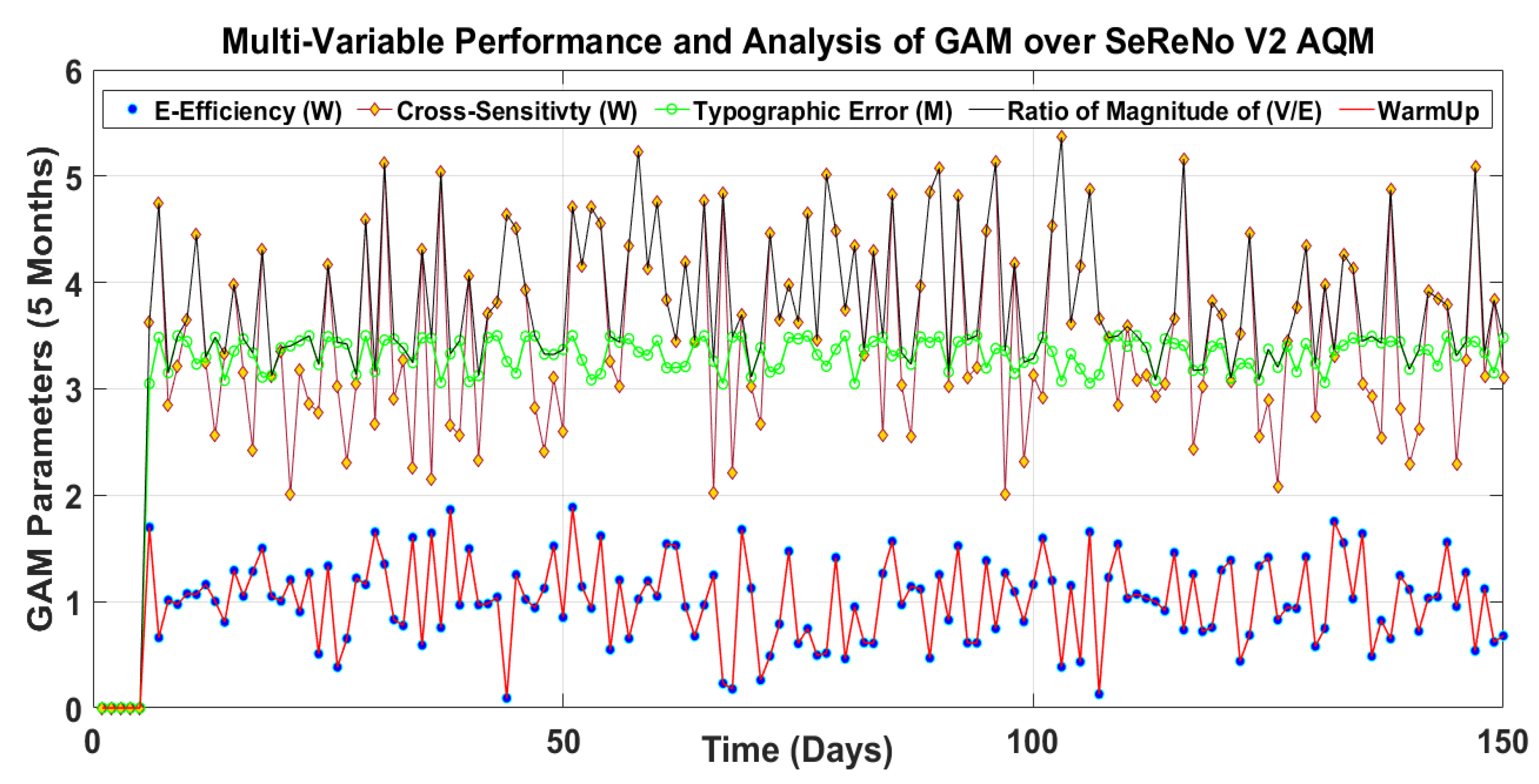
  • The Real-time Gradient Aware Multi-Variable Sensing Model (GAM-VSM)
  • The Optimized Bi-Cluster Regression Machine Learning Model (OBR-MLM)
  • Case Study: Urban Scale IoT-based AQI Monitoring System.
The list of acronyms is presented in Table 2 given below.

2. Materials and Methods

The materials in this work are comprised of a real-time air quality monitoring system and the methods consist of GAM-VSM and OBRM-MLM. The results section gives further insights into this contribution

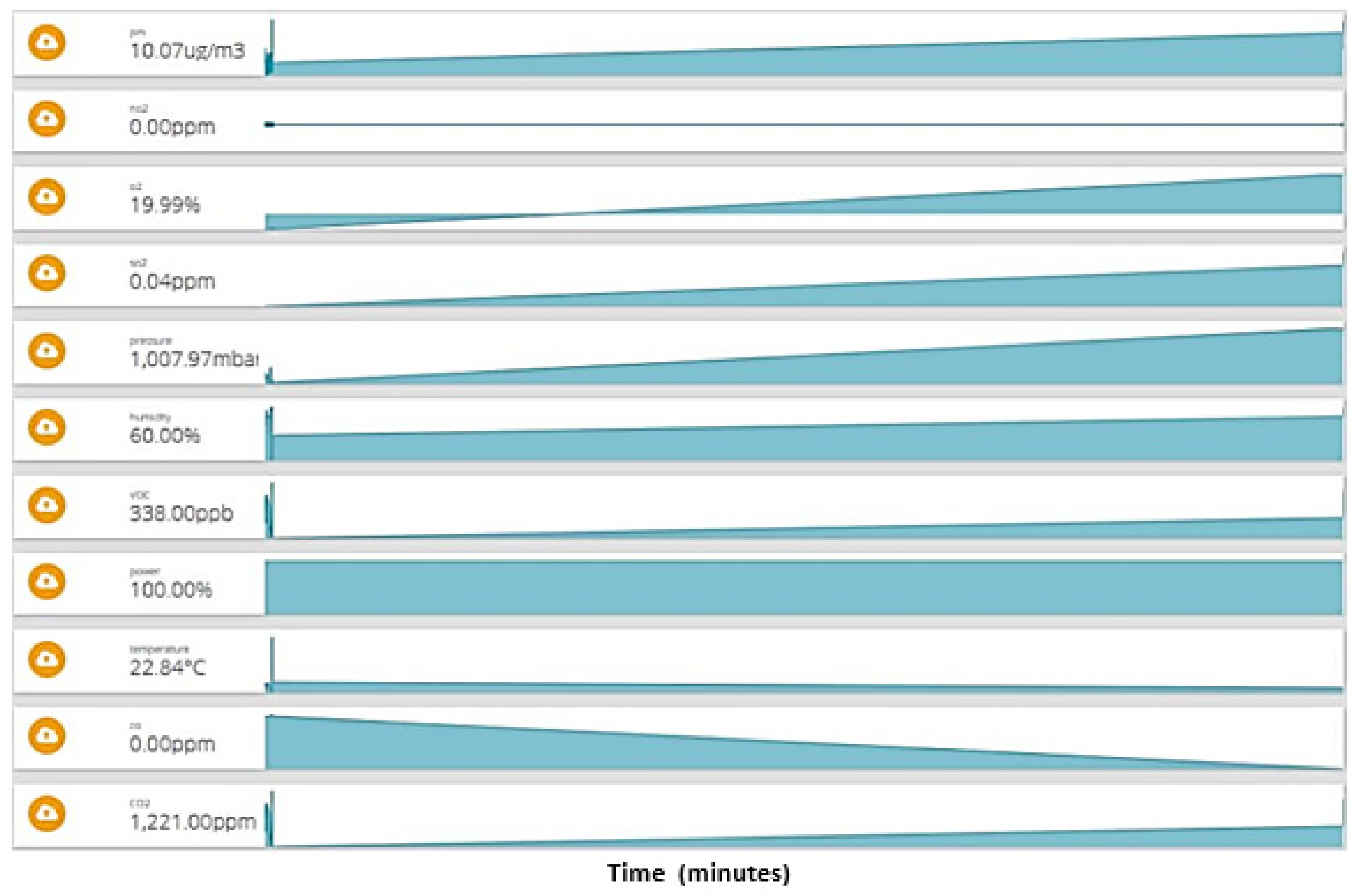
2.1. The Real-Time Multi-Variable Geospatial Gradient-Aware AQI Sensing Model (GAM-VSM)

To measure the precise impact of CO2 and temperature on COVID-19, a real-time multi-variable structured data time-series vector was needed to proceed with the geospatial profiling of gradient awareness as per our past work [25,26]. Let us consider an EPA standard outdoor air quality index (O-AQI) real-time variables as temperature T in centigrade, pressure P in pascals, humidity H in %, volatile organic compounds VoC (ppm), particulate matter as PM (ppm), Ozone as O3 (ppm), Nitrogen Dioxide as NO2 (ppm), Carbon Monoxide as CO2 (ppm), and Sulphur Dioxide as SO2(ppm). The real-time O-AQI data was proposed as a commutative time series multi-variable vector VO-AQI of two non-linear time-series with t1 and t2 of environmental E and gas G sensors data at a particular geo-location L, given as:
VO-AQI (t) = [E(t1), G(t2)]: L(t)
where t = (0, 1, 2, 3, …}
The practicality of the response time of the heterogeneous sensors was taken into account for the non-linear time-series decomposition t, with the gas sensor response time t2 being greater than the response time of environmental sensors t1 with a relationship t2 > t1 given as:
t2 = 3t1
where [t1, t2] ϵ t
The environmental sensor variables function E for sensor array AE (T, P, H, VoC, PM) as E (AE, t1); and gas sensors array AG (O3, NO2, SO2, CO) as G(AG, t2) and position vector L as reference function GPS using GSM network cell locations (using AT + CIPGSMLOC = (1, 1)) for LGPRS and GPS module as LGPS (using AT + CGPSINF). For precise AQM the LGPS must belong to the slope of LGPRS1 and LGPRS2 in a particular slope format by NEMEA specifier for consecutive cells and is given as:
LGPS (X, Y) ϵ [LGPRS1(X2, Y2), LGPRS2(X1, Y1)]
The agreed LGPS was termed as L(t) where condition (3) was satisfied. From Equations (1)–(3) the finalized AQM vector of VO-AQI was derived as:
VO-AQI (t) = [E(AE(T, P, H, VoC, PM),t1), G(AG(O3, NO2, SO2, CO), t2)]: L(t)
Three bounded value conditions were applied on GAM programmed in the SeReNo V2 firmware are presented in Figure 1:
(a)
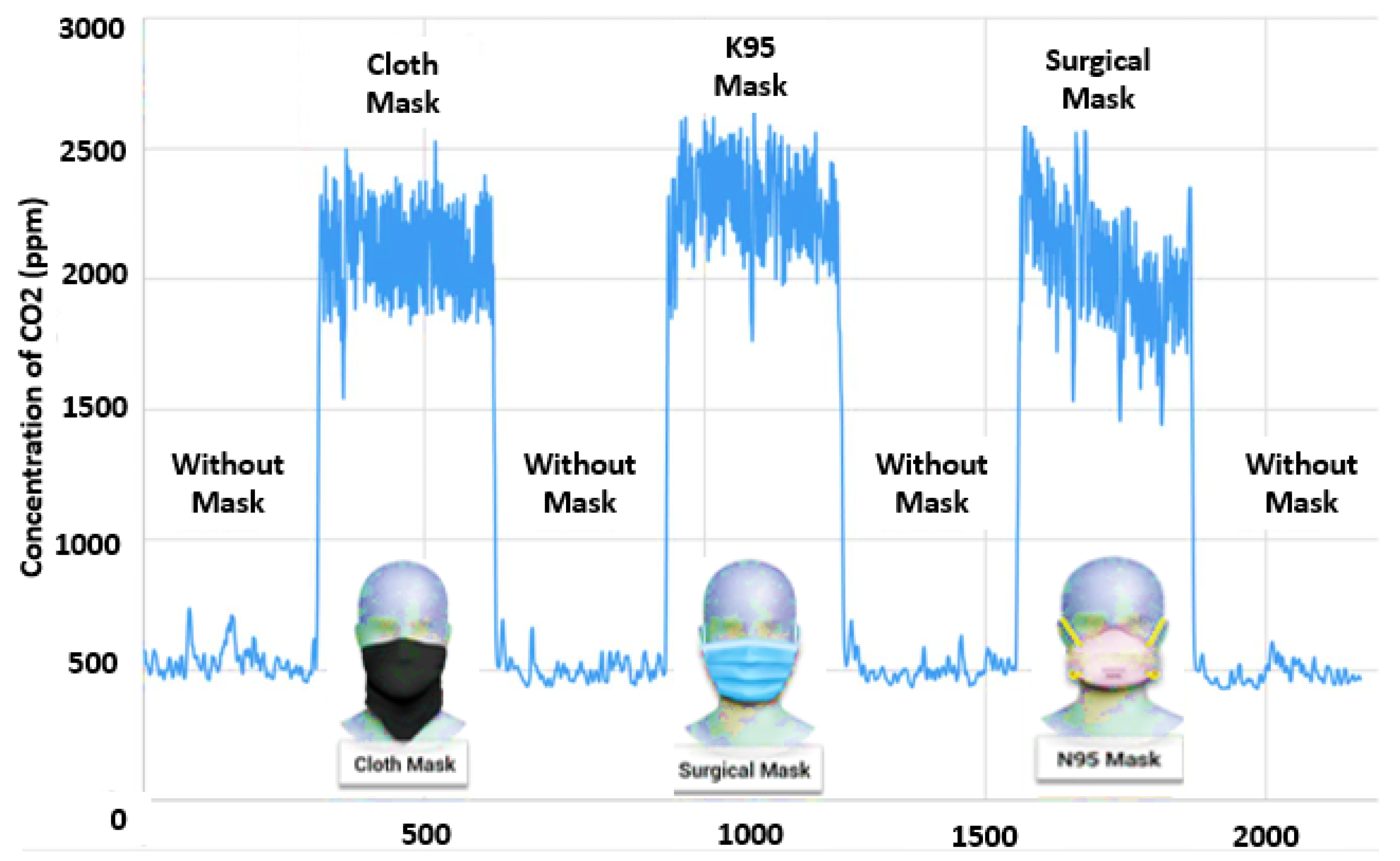
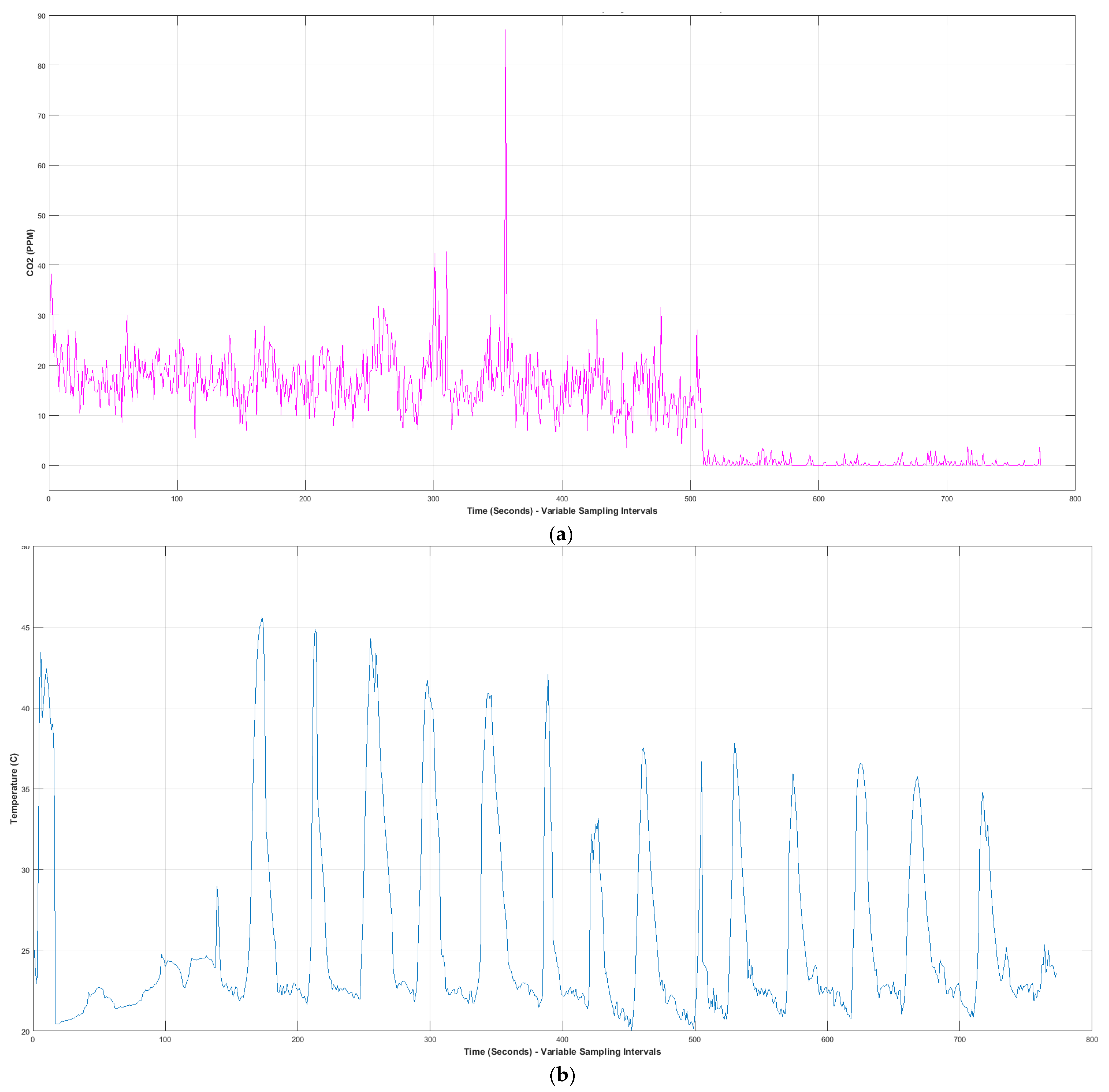
The mandatory gradient unit Δ1CO2 to monitor the CO2 gradient from inhaled air at temperature Δ1T.
(b)
The role of the gradient of the temperature of exhaled air Δ2T with Δ2CO2 recycled in the breathing zone due to a mask.
The optimization scalar is presented as (CO2 is in ppm):
Mask(ΔCO2) = Δ1CO2 × Δ1T + Δ2CO2 × Δ2T

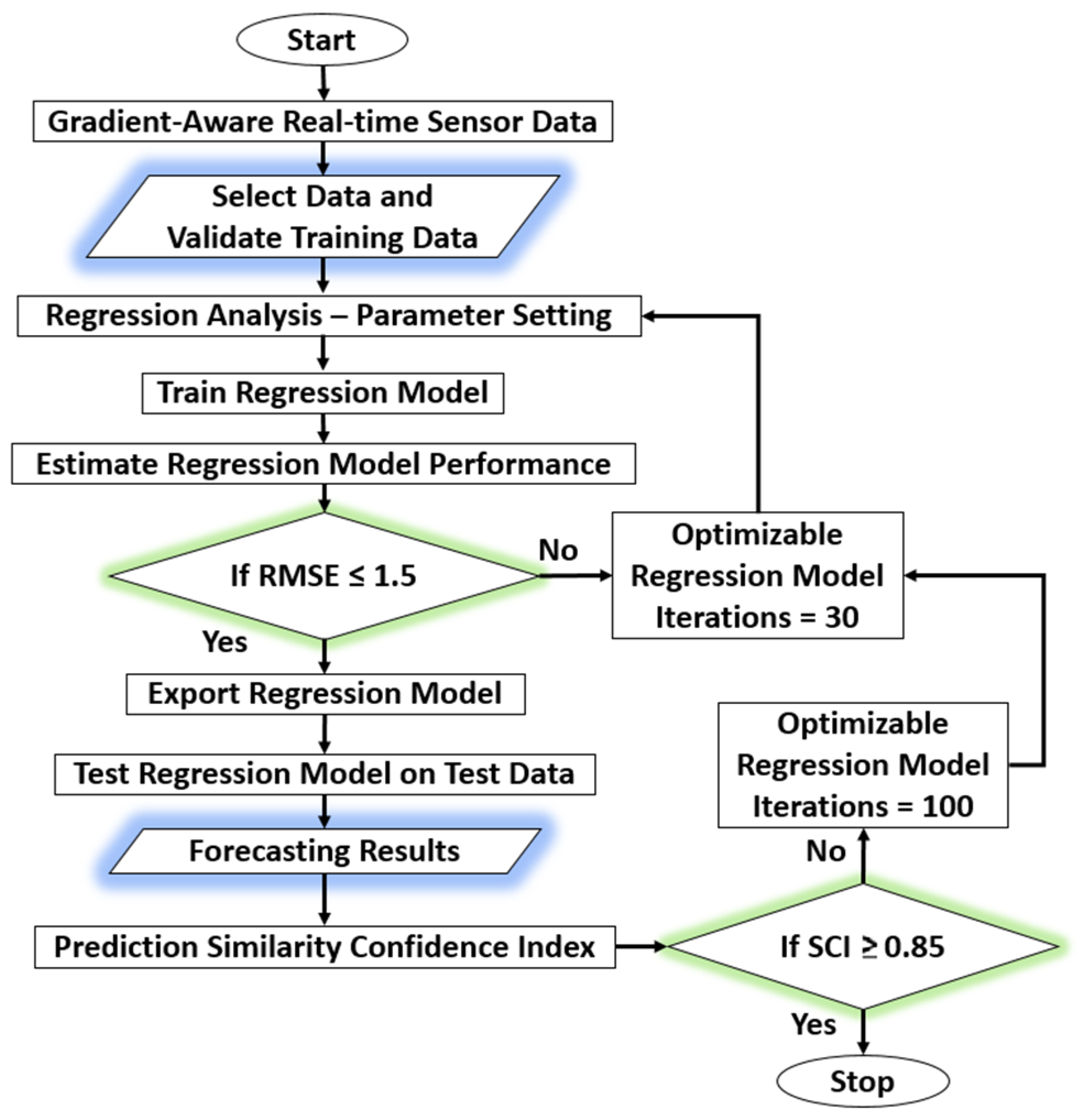
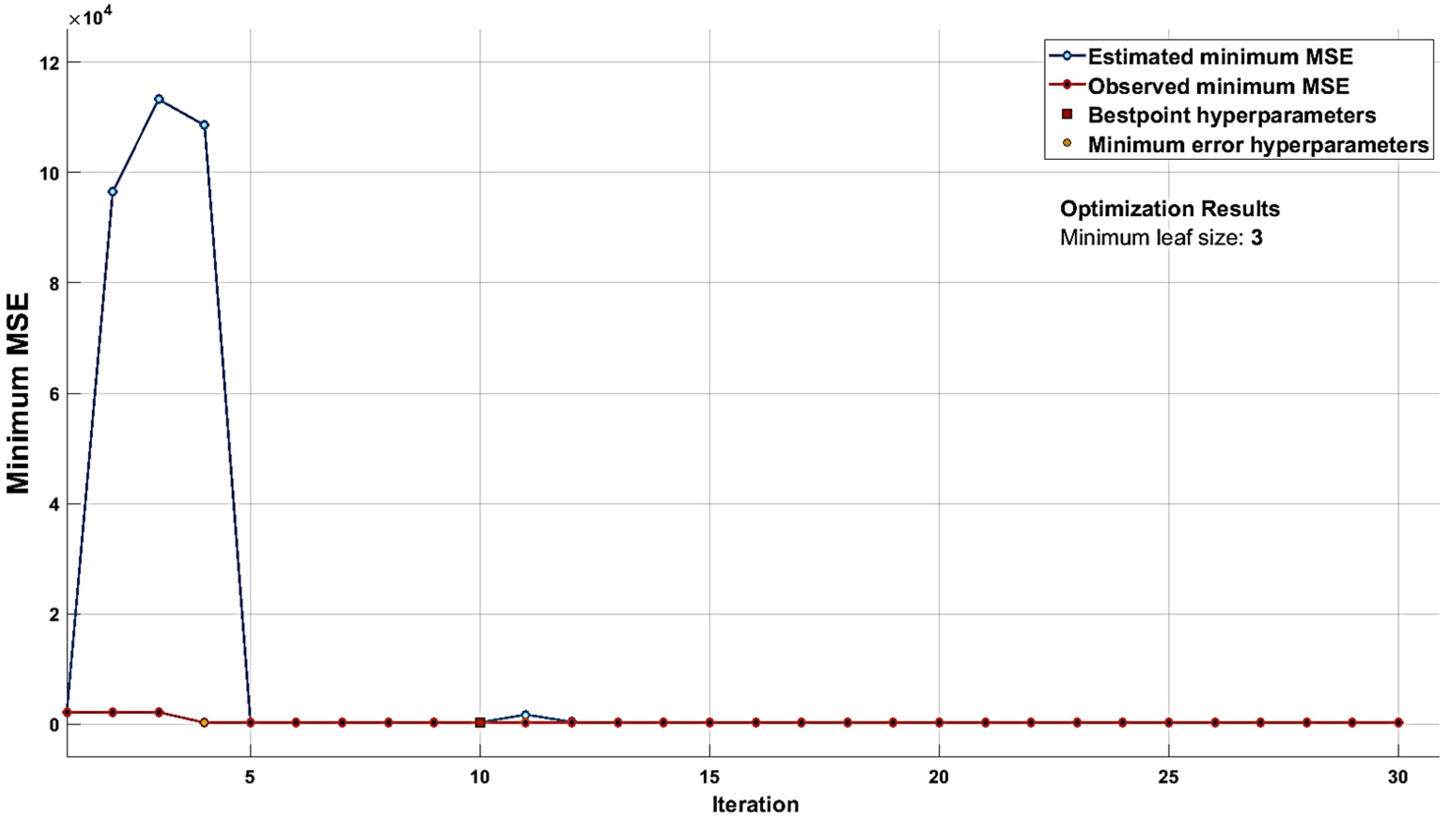
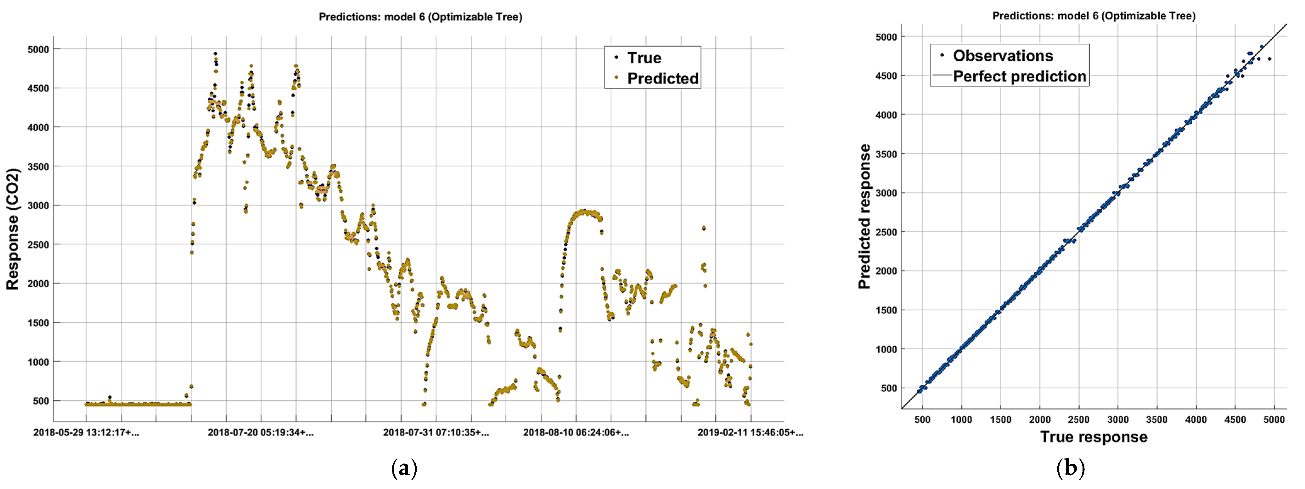
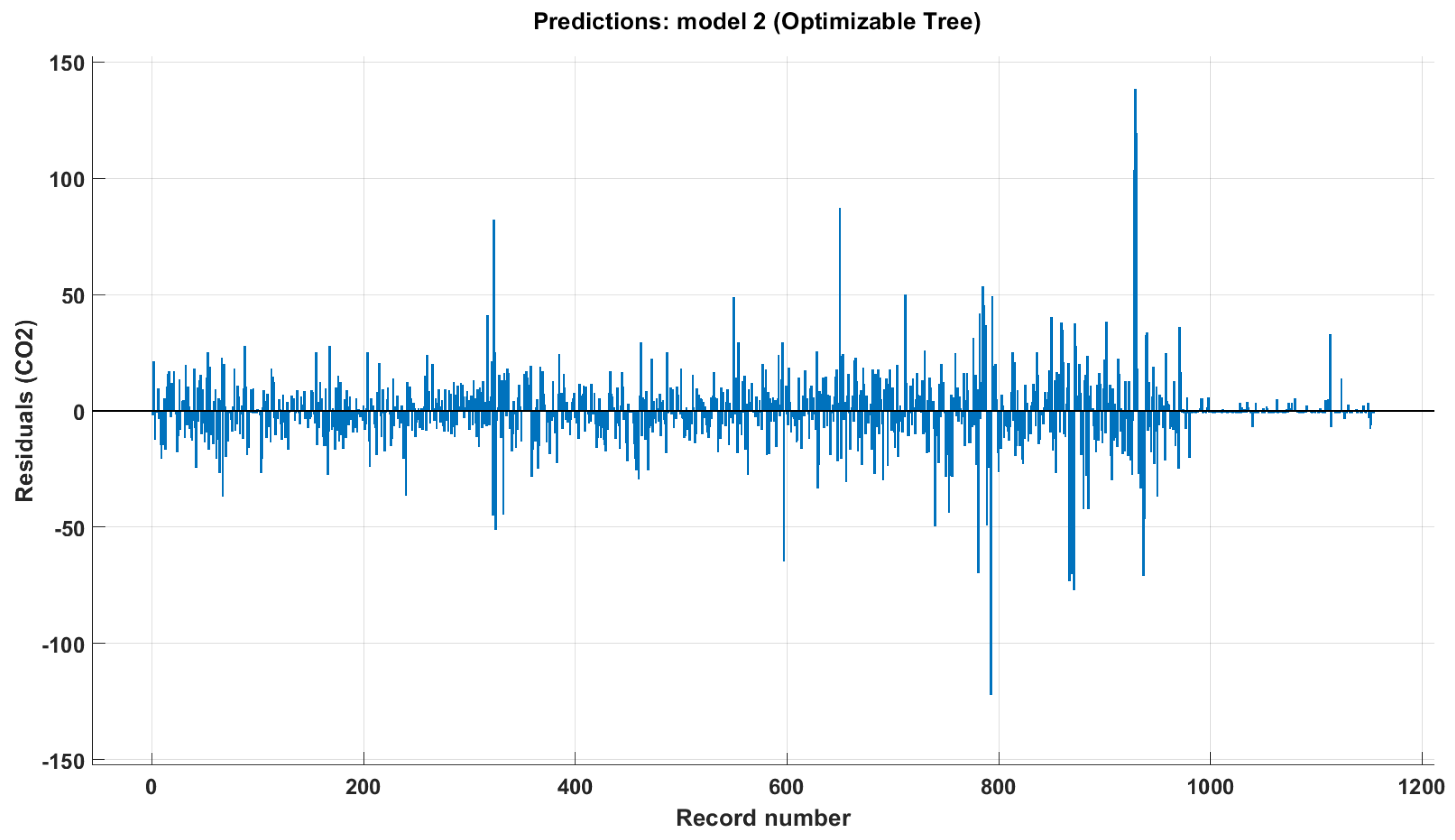
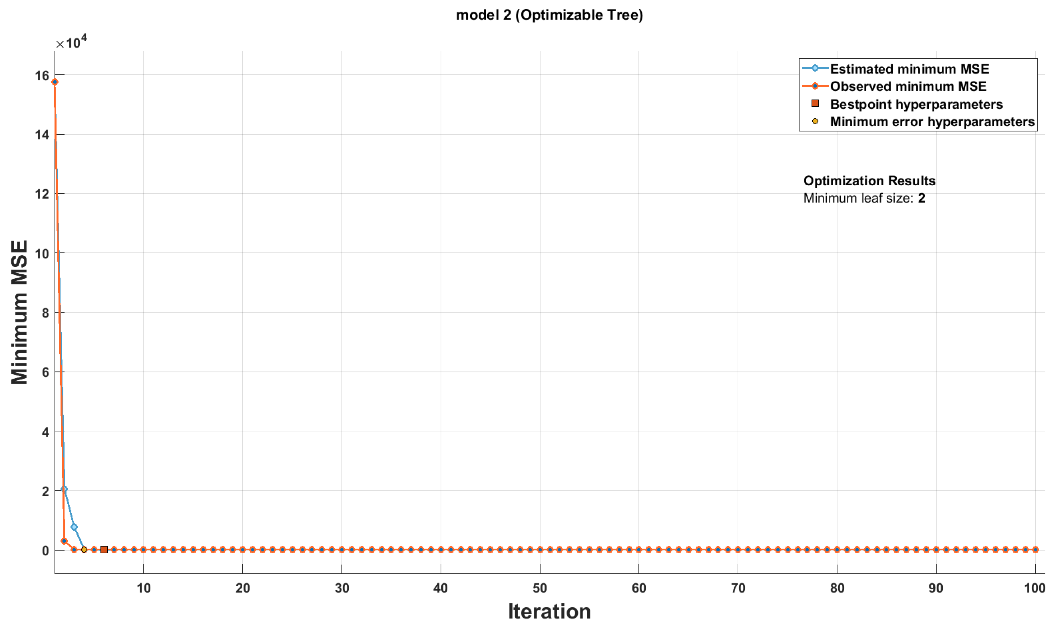
2.2. The Optimized Bi-Cluster Regression Machine Learning Model (OBR-MLM)

The GAM reduced the bulk time-series curation operations needed for forecasting. The dual time-series data was queued to OBRM with (AQI, CO2) and (AQI, Temperature) vectors at the same time with the t1 and t2 time series. The iterative regression parameter setting was performed based on default parameters (RMSE, RSS, and MAE). On every cycle, these parameters were optimized as per the KPI requirements. The two simultaneous regression models were trained for AE(t1) and AG(t2) vectors. The root-mean-square error (RMSE), and mean absolute error (MAE) were the common KPIs that were analyzed before model approval. The approved model was set for forecasting from the SeReNoV2 test data and disapproved data was fed to an optimizer that used a configurable tree-based machine learning approach by variable iterations based on the similarity coefficient index (SCI). The generic regression model Y for
Yt = m = 1 i β m X m , t + ε   = β 1 X 1 , t + β 2 X 2 , t + + β iX i , t + ε
The flowchart of OBRM is presented in Figure 2 below.
As per the proposed bi-cluster networked forecasting of the regression models Yt-CO2 (AQI, CO2) and Yt-Temperature (AQI, Temperature), the regression models must have an acceptable similarity of >85%. If the forecasted time-series curves from two similar sensors installed at two different locations have curve-similarity concerning their AQI curves, termed as similarity coefficient index (SCI) as less than 85%, the iterations will keep running automatically. For RMSE < 1.5, statistically the SCI < 0.85 conditions should be satisfied in real-time. The US EPA AQI standard for outdoor air quality is presented in Table 3 below:
The AQI is generically estimated as:
I P = [ ( I h i g h I l o w ) / ( B P - h i g h -   B P - l o w ) ] × ( C P B P l o w ) + I l o w
Every pollutant was formulated using Equation (7) and given by Equations (8) to (12).
I P M = [ ( I h i g h I l o w ) / ( B P M h i g h B P M l o w ) ] × ( C P M B P M l o w ) + I l o w
I NO 2 = [ ( I h i g h I l o w ) / ( B NO 2 h i g h B NO 2 l o w ) ] × ( C NO 2 B NO 2 l o w ) + I l o w
I SO 2 = [ ( I h i g h I l o w ) / ( B SO 2 h i g h B SO 2 l o w ) ] × ( C SO 2 B SO 2 l o w ) + I l o w
I O 3 = [ ( I h i g h I l o w ) ( B O 3 h i g h B O 3 l o w ) ] × ( C O 3 B O 3 l o w ) + I l o w
  I C O = [ ( I h i g h I l o w ) / ( B C O h i g h B C O l o w ) ] × ( C C O B O 3 l o w ) + I l o w
From the AQI equations the resulting relative regression models for CO2 ( I m CO 2 , t ) and Temperature ( I m T , t ) are given as:
Y t - CO 2 = m CO 2 = 1 i β m CO 2 I m CO 2 , t + ε CO 2
= β1-CO2I1-CO2,t + β2-CO2I2-CO2,t + … + βi-CO2 I i - CO 2 , t + ε CO 2
Y t - T = m T = 1 i β m T I m T , t + ε T   I i - T , t + ε T
= β1-TI1-T,t + β2-TI2-T,t + … + βi-TIi-T,t + εT
The function Iµ has been used to express the rate of change in AQI at the corresponding time derivative.
( I µ ) n = Δ AQI Δ t = 2 k r e 2   ( 1 + e r t ) 2 × t + = 0 ,   1 ,   2
To compare the relative influence level among the various influencing factors, the regression coefficients were normalized.
β m = β m × σ Xm σ Y
where β’m is the normalized regression coefficient of the mth driving force, and βm is the regression coefficient of the driving force. σXm is the standard deviation of the driving force, and σY is the standard deviation of the dependent variable. The RMSE will be the first step in ML model testing and optimization and is given as:
RMSE = 1 n i = 1 n ( M i R M i ) 2
This indicates the magnitude of the error and retains the variable’s unit; is sensitive to extreme values and outliers; tends to vary as a function of the standard deviation of the RM. Based on the RMSE the iteration will be performed by eliminating the temperature effect ET and CO2 ECO2 effect respectively from Equations (13) and (14) using:
E T = n i = 1 n Y i T C i i = 1 n Y i T i = 1 n C i n i = 1 n ( Y i T ) 2 ( i = 1 n Y i T ) 2
E CO 2 = n i = 1 n Y i CO 2 C i i = 1 n Y i CO 2 i = 1 n C i n i = 1 n ( Y i CO 2 ) 2 ( i = 1 n Y i CO 2 ) 2
sensitivity coefficient C for the measurement influencing variable and finally:
RSS = i = 1 ( γ i - b 0 b 1 x i ) 2
The RSS is measured as the sum of the square of residuals as the final step in the iterative optimization. In the results section, an ambient role of magnitudes of two variables can be observed, but the RMSE and MAE are not enough to resolve the sensor data with different scales and orders of magnitude for this SCI. The SCI for CO2 (SCICO2) and temperature (SCIT) will be the tacking gradient (real-time difference divided by their average) ratio of two cluster nodes 1 and 2 given as:
  SCI CO 2 = 2   ×   | SCI CO 2 - 1 -   SCI CO 2 - 2 SCI CO 2 - 1 + SCI CO 2 - 2 |
  SCI T = 2   ×   | SCI T - 1 -   SCI T - 2 SCI T - 1 + SCI T - 2 |
  SCI = β m   ×   | ( SCI T   ×   E CO 2 ) + ( SCI T × E CO 2 ) 2 |
The present probability of infection (PInfection-Present) is based on present data and the future probability of infection (PInfection-Future) is based on forecasted data. Based on previous research mentioning the COVID-19 relationship with temperature and CO2 and Mask(ΔCO2) (cycling the CO2 into the lungs that gradually weakens the lungs) from Equation (5) and relative influence level based on β′m (Equation (16)) the probability (PInfection) of trans-respiratory pandemics and COVID-19 is given by:
P Infection - Present = | SCI RMSE   ×   I µ |
P Infection - Future = ( P Infection - Present × 1   I µ ) + ( Mask ( Δ CO 2 ) × | Y t - CO 2 Y t - T | )
The proposed automated iterative optimization for COVID-19 and other pandemics that are based on some sensing variables is independent of personal immunity and the infection capability or the strength of pathogens as a medical science research area.

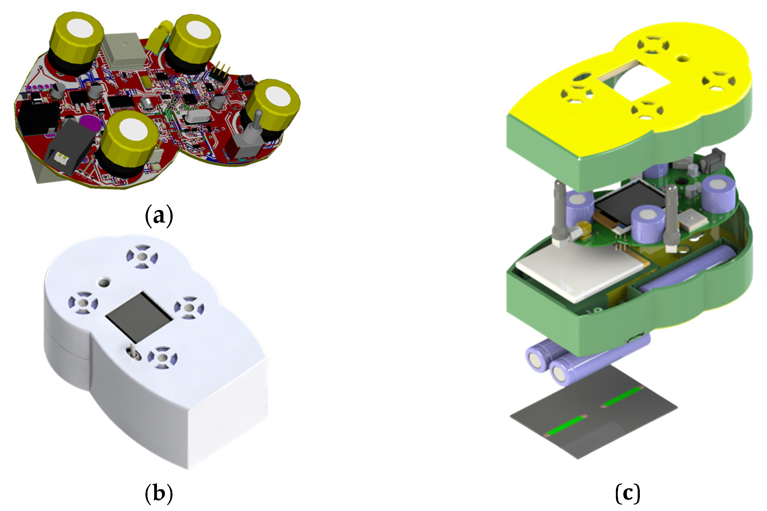
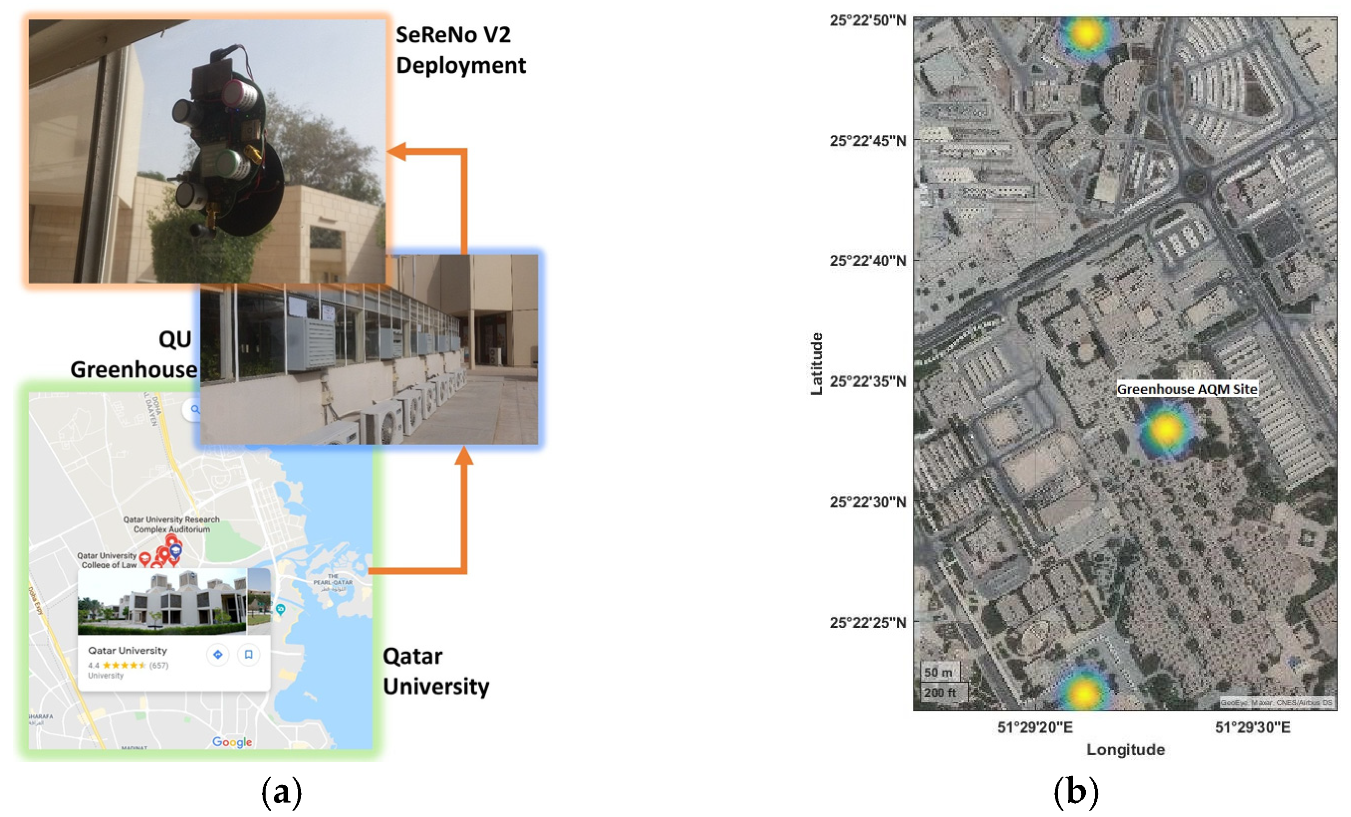
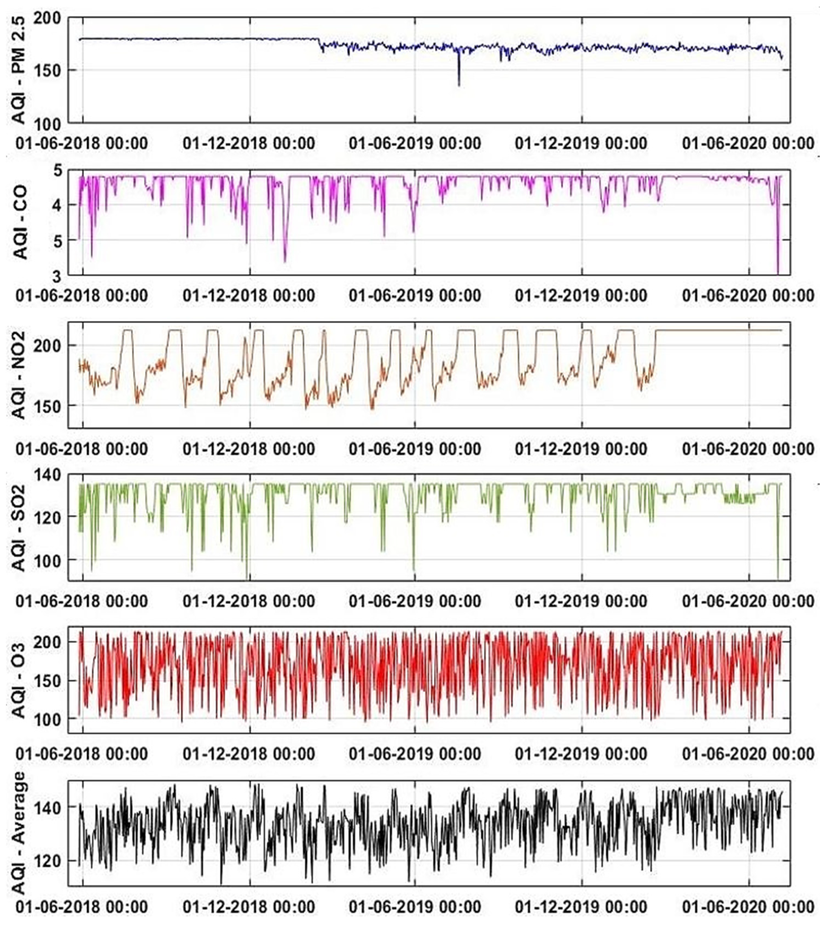
2.3. A Case Study: Urban Scale IoT-Based AQI Monitoring System

The proposed model and applied algorithm were tested and validated using our TRL7 autonomous AQI mapping system from past research [25,26]. A 1-1 correspondence electronics and instrumentation system was designed in a single package, i.e., SeReNoV2 presented in Figure 3 presented below.
Three SeReNo V2 nodes were fabricated and deployed in QU for outdoor testing. The fabricated SeReNo V2 was deployed based on the efficient utilization of GAM, i.e., QU Greenhouse exhibited in the Figure 4 below.
The GAM reduced the bulk time-series curation operations needed for forecasting. The dual time-series data was queued to OBRM with (AQI, CO2) and (AQI, Temperature) vectors at the same time with the t1 and t2 time series. The iterative regression parameter setting was performed based on default parameters (RMSE, RSS, and MAE). On every cycle, these parameters were optimized; AQI refers to a structured chart with a bio-tolerable threshold of specific pollutants and bio-hazardous gases recommended by EPA in the area under a specified border agency18–24. The top 10 environmental protection agencies (EPAs) unanimously agreed on the standard of four core gases for outdoor.

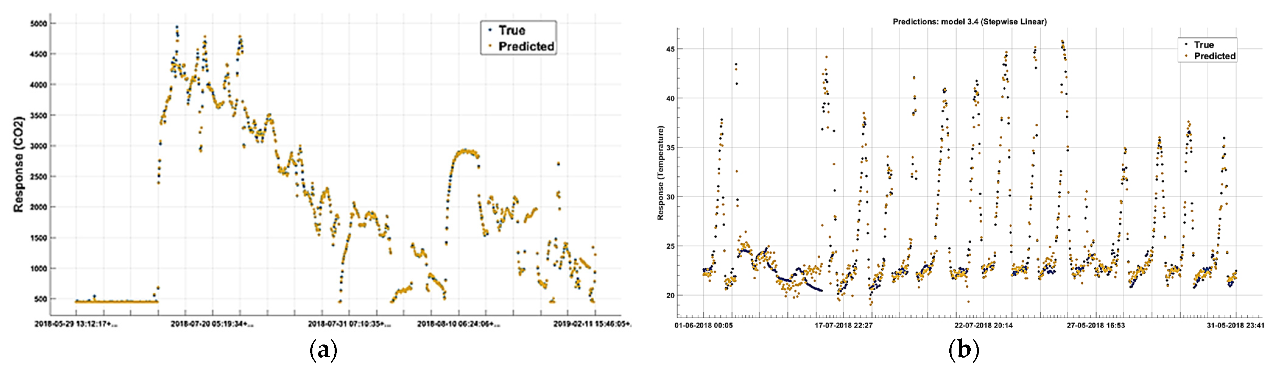
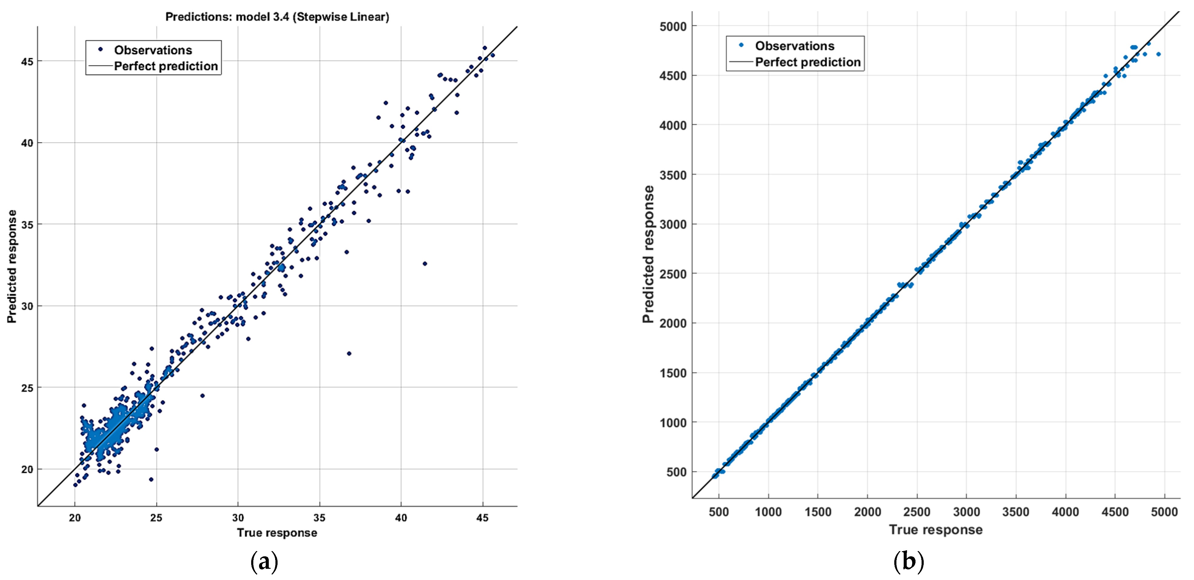
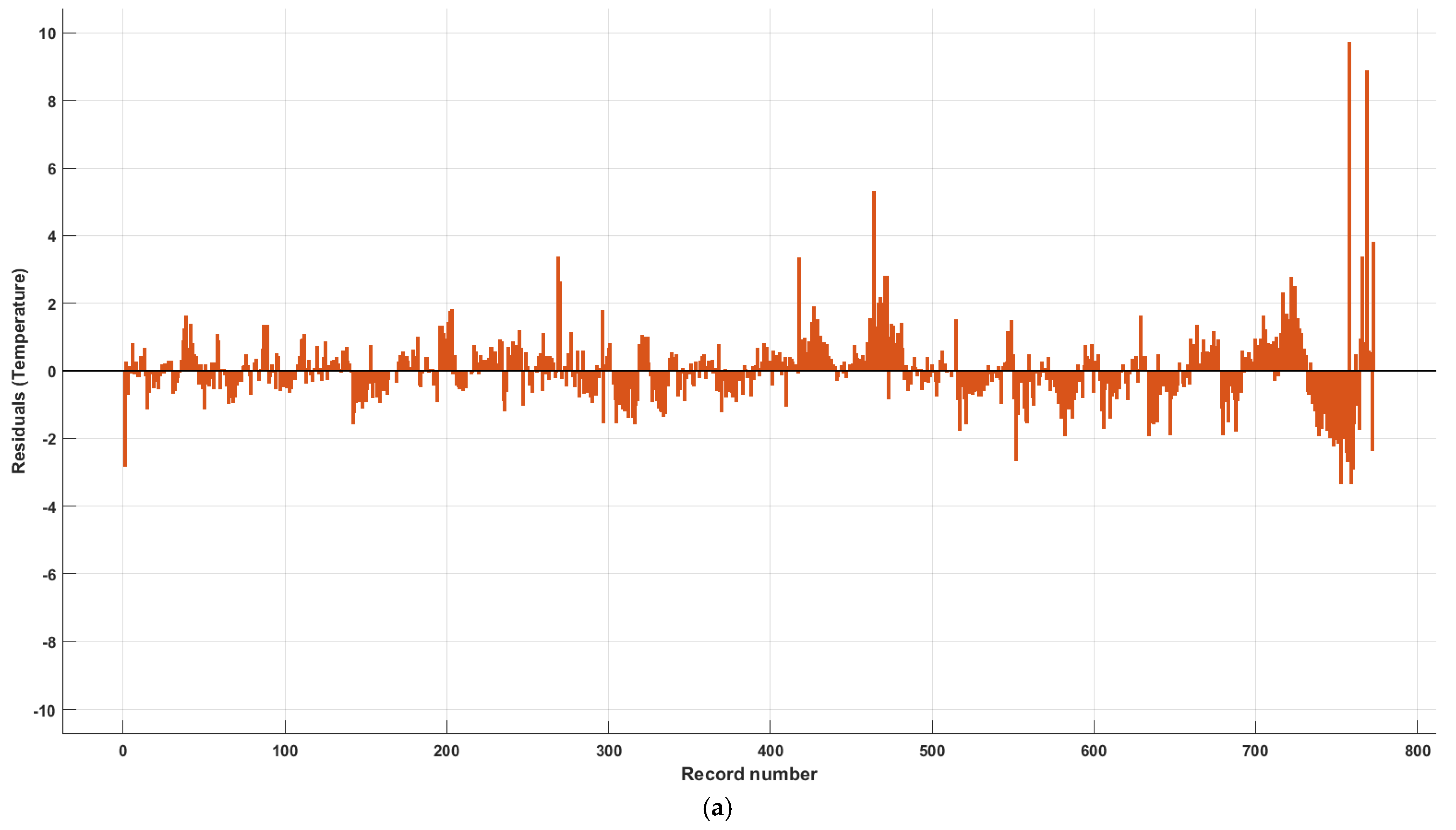
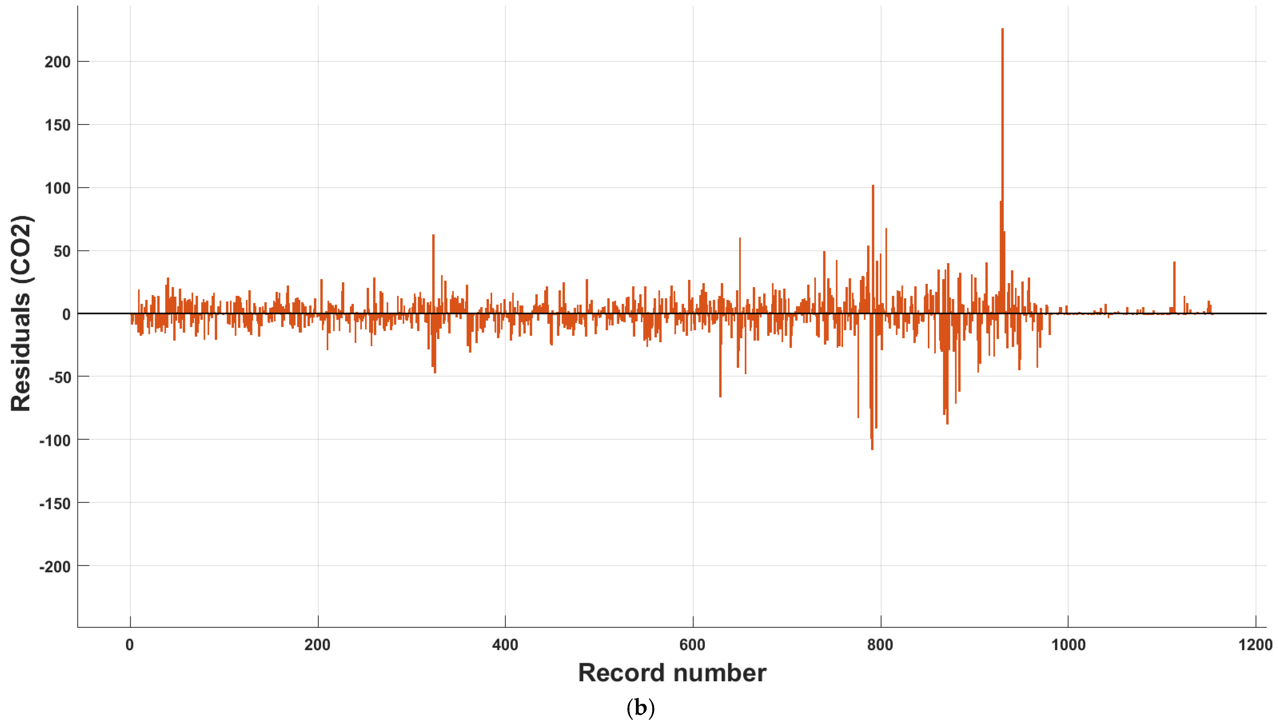
3. Results and Discussion

After the long-haul deployment of six months, the data results obtained were displayed on the Ubidots IoT platform as shown in Figure 5.
The eleven real-time variables were exhibited in Figure 4, sending data through the GSM model QuecTel M10. The bi-cluster is considered in this special data-fusion case for data collected at the central site, i.e., QU Greenhouse. The two variables CO2 and temperature were double interpolated from four sites (top: QU H10 and QU C05) and presented in Figure 6 below from the Ubidots IoT platform.
Since trans-respiratory diseases, as per WHO and US EPA, get worst due to poor AQI, from (8) to (12) the Cumulative AQI of four sites is given in Figure 7.
The application of GAM enabled only meaningful data to be sent to the cloud, which made the time series more non-linear as only gradient-impacted values were being transmitted. The accuracy of bi-clustered data measurements in terms of the autonomous AQI system by applying our previous work is exhibited in Figure 7. The following plots of individual variables give more insight into GAM in the SeReNoV2. The KPIs of GAM contributed to the accuracy and efficiency of the OBRM.
The impact of GAM can be warm times below 1.83 s throughout 5 months. The reduced warm-up times reduce the boot time power spike and result in the stable voltage above 3.3 V needed for the sensors. The typographic error observed is around 3.1 to 3.4, which is much less. A minute typographic error can be observed due to the correlation of the GPS and GPRS-assisted cell network locations scheme. The key performance indicators (KPIs) of GAM efficiency on SeReNoV2 were the major contribution that enabled all the outcomes presented in Figure 8, Figure 9, Figure 10, Figure 11, Figure 12, Figure 13, Figure 14, Figure 15, Figure 16 and Figure 17, as detailed in Figure 17.
The dual-time series regression of OBRM is presented as CO2 being the top concern in Qatar. This outcome contributed to potential safety precautions during COVID-19. A four-step procedure was followed for OBRM. First, the predicted response was assessed and the ML KPIs, mentioned in Table 1, were streamlined. Then the comparison was performed between real and predicted; at this step, the trained model residuals were estimated and finally, the optimization was performed as per conditions.
Figure 9a exhibits the temperature response for model 1, termed OBRM1. The real data is in blue and the predicted is in orange. It was measured for one month. The RMSE of 1.0042 was almost ideal and needed no further tuning and verification. Figure 9b is a realization of a close prediction, as the predicted and actual are almost overlapping with RMSE 1.7+.
In Figure 10a, the wrapping of blue markers or bubbles over the ideal or accurate prediction shows the accuracy of the prediction using customized linear regression. Maximum similarity can be observed in magnitudes of 21 °C to 24.5 °C. In the next process, the residual was estimated as the vertical distance between a data point and the regression line. Each data point has one residual. They are positive if they are above the regression line and negative if they are below the regression line. If the regression line passes through the point, the residual at that point is zero.
The RMSE of 1.7+ is extremely small for magnitudes like 6000, thus the comparative plot for the predicted and true is almost overlapping in Figure 10b.
In Figure 11a, the magnitudes of 9+ for residuals are non-convex and impact the error in the prediction by OBRM1 for temperature. The AE(t1) cluster was not optimized due to RMSE 1.0042. The optimization was performed for RMSE > 1.5 for AG(t2), presented in Figure 9, Figure 10, Figure 11 and Figure 12. The residuals for temperature and CO2 are presented in the Figure 11.
The 200 residual magnitudes for amplitudes of PPM like 4500+ are minute, i.e., 200/4500 = 0.044 shown in Figure 11b.
The results in Figure 12 lead to level 2 optimization of the OBRM1 based on the leaf size 3.
The tracking and alignment performed by OBRM3 for the observed and predicted CO2 (PPM) is up to 4400 ppm in Figure 13.
The offset or residual of 150/4800 = 0.03125 ppm is almost perfect or accurate as examined in Figure 14. The 200 residual magnitudes for amplitudes of PPM like 4500+ are minute, i.e., 200/4500 = 0.044 shown in Figure 14.
The leaf size of 2 with 100 iterations delivered fine-tuned optimization and tracking for the precise prediction observed in Figure 16. Later, the generated model was tested over test data for predicting the CO2 for the years 2021 and 2022. This is presented in Figure 16.
The PInfection-Future for CO2 by OBRM3 was almost similar; it was ambient from Figure 16 with a numerical explanation and highlights for SCI computation. The OBRM3 had a very minute difference between the present and forecasted data.
The parameter setting for an optimized linear regression and optimized tree are presented in Table 4. The training time and predicted speed are related as they are reciprocal to each other.
The probability of errors in the magnitude range set {0.06, 0.15} is 0, observed in Figure 17. A comparison of the results with other studies was not possible, as shown in Table 1, because none of the past studies used real-time sensor data forecasting for two time-clustered IoT node measurements, and so these results are exclusively based on our data.

4. Limitations and Future Recommendation

This experiment and study were based on AQI sensing at different locations within Qatar University. The 4 SeReNo V2 AQI sensors nodes were in two buildings with similar conditions and two buildings with different conditions. A dual installation was performed to avoid any measurement errors, as per Figure 9, based on previous studies (Hasan et al., 2020). Since the trans-respiratory pandemics, especially COVID-19, are more impactful at gatherings and populated premises, the university was chosen and the equations and their respective figures provided a precise route map of forecasting. Based on Equations (24) and (25) using SCI, countermeasures can be easily taken by raising the temperature to the un-survivable limit for COVID-19 pathogens and by using CO2-capturing units and O2 cylinders to cycle fresh air.
This study will be more impactful if such AQI nodes are installed in hospitals and measured for COVID-19-tested positive and negative patients. Our research group is looking forward to conducting this research in hospitals which was not possible during the pandemic times due to social isolation.

5. Conclusions

A novel similarity coefficient index-based forecasting method for COVID-19 and trans-respiratory pandemics is proposed using the SeReNoV2 nodes. A multi-time series-parallel automated iterative optimization of regression models was performed with interesting results. The presented work highlighted the practical time-series challenge of duality and multi-cluster vector forecasting for COVID-19 safety with the impact of masks. To the best of our knowledge, this is the first real-time bi-cluster dual time-series forecasting machine learning approach for real-time multi-source sensor temporal data forecasting. The results can be summarized in three key milestones. The optimized regression methodology was able to: (1) implement a dual-time series analysis for a non-linear composite time series vector, compensating for the commutative anomalies in the bi-cluster sensor network; (2) the selected KPIs for the data preprocessing by hardware resulted in reduced training time and improved prediction speeds of the machine learning model training; (3) the forecasted results were overlapping being a justified precision in forecasting methodology accuracy for COVID-19 infections. The proposed method can serve as a role model for dual time-series problems in COVID-19 and other complex pandemics.

Author Contributions

Conceptualization, H.T.; Data curation, H.T.; Formal analysis, H.T.; Funding acquisition, F.T., D.C. and A.B.M.; Investigation, H.T.; Methodology, H.T.; Project administration, F.T.; Resources, F.T., D.C. and A.B.M.; Software, H.T.; Supervision, F.T.; Validation, H.T.; Visualization, H.T.; Writing—original draft, H.T.; Writing—review & editing, F.T., D.C. and A.B.M. All authors have read and agreed to the published version of the manuscript.

Funding

This publication was made possible by NPRP grant # 10-0102-170094 from the Qatar National Research Fund (a member of Qatar Foundation).

Institutional Review Board Statement

Not applicable.

Informed Consent Statement

Not applicable.

Data Availability Statement

The data presented in this study are available on request from the corresponding author.

Acknowledgments

This publication was made possible by NPRP grant # 10-0102-170094 from the Qatar National Research Fund (a member of Qatar Foundation). The statements made herein are solely the re-sponsibility of the authors.

Conflicts of Interest

The authors declare no conflict of interest.

References

  1. Dorota, J. WHO Global Air Quality Guidelines; World Health Organization: Geneva, Switzerland, 2021. [Google Scholar]
  2. US EPA. National Ambient Air Quality Standards (NAAQS); US EPA: Washington, DC, USA, 2020. [Google Scholar]
  3. Liu, Z.; Ciais, P.; Deng, Z.; Lei, R.; Davis, S.J.; Feng, S.; Zheng, B.; Cui, D.; Dou, X.; Zhu, B. Near-real-time monitoring of global CO2 emissions reveals the effects of the COVID-19 pandemic. Nat. Commun. 2020, 11, 5172. [Google Scholar] [CrossRef]
  4. Peng, Z.; Jose, L. Exhaled CO2 as a COVID-19 Infection Risk Proxy for Different Indoor Environments and Activities. Environ. Sci. Technol. Lett. 2021, 8, 392–397. [Google Scholar] [CrossRef]
  5. Jiandong, C.; Chong, X.; Ming, G.; Ding, L. Carbon peak and its mitigation implications for China in the post-pandemic era. Sci. Rep. 2022, 12, 3473. [Google Scholar]
  6. Dias, S.B.; Hadjileontiadou, S.J.; Diniz, J.; Hadjileontiadis, L.J. DeepLMS: A deep learning predictive model for supporting online learning in the COVID-19 era. Sci. Rep. 2020, 10, 19888. [Google Scholar] [CrossRef] [PubMed]
  7. Zhou, Y.; Jinyan, Z.; Shanying, H. Regression analysis and driving force model building of CO2 emissions in China. Sci. Rep. 2020, 11, 6715. [Google Scholar] [CrossRef] [PubMed]
  8. Malik, A.; Kumar, A. Spatio-temporal trend analysis of rainfall using parametric and non-parametric tests: Case study in Uttarakhand, India. Theor. Appl. Climatol. 2020, 140, 183–207. [Google Scholar] [CrossRef]
  9. Abbasi, S.A. Monitoring analytical measurements in presence of two component measurement error. J. Anal. Chem. 2014, 69, 1023–1029. [Google Scholar] [CrossRef]
  10. Santiago, M.-C.; Eugenio, F.; Antonio, M. Time Series Decomposition of the Daily Outdoor Air Temperature in Europe for Long-Term Energy Forecasting in the Context of Climate Change. Energies 2020, 13, 1569. [Google Scholar]
  11. Stanislaus, S.U. Power Comparisons of Five Most Commonly Used Autocorrelation Tests. Pak. J. Stat. Oper. Res. 2020, 16, 119–130. [Google Scholar]
  12. Ian, F.A.; Weilien, S.; Yoegsh, S.; Erdal, C. A Survey on Sensor Networks. IEEE Commun. Mag. 2002, 40, 102–114. [Google Scholar]
  13. Tariq, H.; Shafaq, S. Real-time Contactless Bio-Sensors and Systems for Smart Healthcare using IoT and E-Health Applications. WSEAS Trans. Biol. Biomed. 2022, 19, 91–106. [Google Scholar] [CrossRef]
  14. Touati, F.; Tariq, H.; Mohammed, A.A.; Adel, B.M.; Anas, T.; Damiano, C.I. IoT and IoE Prototype for Scalable Infrastructures, Architectures and Platforms. Int. Robot. Autom. 2018, 4, 319–327. [Google Scholar] [CrossRef] [Green Version]
  15. Vinyals, M.V.; Juan, R.-A.; Jesús, C. A Survey on Sensor Networks from a Multi-Agent Perspective. Comput. J. 2014, 54, 455–470. [Google Scholar]
  16. Saberi-Movahed, F.; Mohammadifard, M.; Mehrpooya, A.; Rezaei-Ravari, M.; Berahmand, K.; Rostami, M.; Karami, S.; Najafzadeh, M.; Hajinezhad, D.; Jamshidi, M. Decoding clinical biomarker space of COVID-19: Exploring matrix factorization-based feature selection methods. Comput. Biol. Med. 2022, 146, 105426. [Google Scholar] [CrossRef]
  17. Tariq, H.; Tahir, A.; Touati, F.; Al-Hitmi, M.; Mnaouer, A.B.; Crescini, D. Structural Health Monitoring and Installation Scheme deployment using Utility Computing Model. In Proceedings of the 2018 2nd European Conference on Electrical Engineering and Computer Science (EECS), Bern, Switzerland, 20–22 December 2018. [Google Scholar] [CrossRef]
  18. Mehrpooya, A.; Saberi-Movahed, F.; Azizizadeh, N.; Rezaei-Ravari, M.; Eftekhari, M.; Tavassoly, I. High dimensionality reduction by matrix factorization for systems pharmacology. Brief. Bioinform. 2021, 23, bbab410. [Google Scholar] [CrossRef]
  19. Tariq, H.; Touati, F.; Al-Hitmi, E.; Crescini, D.; Mnaouer, A.B. Design and Implementation of Programmable Multi-parametric 4-Degrees of Freedom Seismic Waves Ground Motion Simulation IoT Platform. In Proceedings of the 2019 15th International Wireless Communications & Mobile Computing Conference (IWCMC), Tangier, Morocco, 24–28 June 2019. [Google Scholar] [CrossRef]
  20. Sadeghi, G.; Najafzadeh, M.; Ameri, M.; Jowzi, M. A case study on copper-oxide nanofluid in a back pipe vacuum tube solar collector accompanied by data mining techniques. Case Stud. Therm. Eng. 2022, 32, 101842. [Google Scholar] [CrossRef]
  21. Najafzadeh, M.; Oliveto, G. More reliable predictions of clear-water scour depth at pile groups by robust artificial intelligence techniques while preserving physical consistency. Soft Comput. 2022, 25, 5723–5746. [Google Scholar] [CrossRef]
  22. Tariq, H.; Abdarazzak, A.; Farid, T.; Mohammed, A.E.A.; Damiano, C.; Adel, B.M. An Autonomous Multi-Variable Outdoor Air Quality Mapping Wireless Sensors IoT Node for Qatar. In Proceedings of the 2020 International Wireless Communications and Mobile Computing (IWCMC), Limassol, Cyprus, 15–19 June 2020. [Google Scholar] [CrossRef]
  23. Geiss, O. Effect of Wearing Face Masks on the Carbon Dioxide Concentration in the Breathing Zone. Aerosol Air Qual. Res. 2021, 21, 200403. [Google Scholar] [CrossRef]
  24. Michelle, S.M.; Carin, D.L.; Matthew, T.; Amanda, C.; Jonathan, J.Y. Carbon dioxide increases with face masks but remains below short-term NIOSH limits. BMC Infect. Dis. 2021, 21, 354. [Google Scholar]
  25. Tariq, H.; Abdaoui, A.; Touati, F.; Al-Hitmi, E.; Crescini, D.; Mnaouer, A.B. Real-time Gradient-Aware Indigenous AQI Estimation IoT Platform. Adv. Sci. Technol. Eng. Syst. J. 2020, 5, 1666–1673. [Google Scholar] [CrossRef]
  26. Tariq, H.; Abdaoui, A.; Touati, F.; Al-Hitmi, E.; Crescini, D.; Mnaouer, A.B. A Real-time Gradient Aware Multi-Variable Handheld Urban Scale Air Quality Mapping IoT System. In Proceedings of the IEEE International Conference on Design & Test of Integrated Micro & Nano-Systems (DTS), Hammamet, Tunisia, 7–10 June 2020. [Google Scholar] [CrossRef]
  27. Elbeltagi, A.; Al-Mukhtar, M.; Kushwaha, N.L.; Al-Ansari, N.; Vishwakarma, D.K. Forecasting monthly pan evaporation using hybrid additive regression and data-driven models in a semi-arid environment. Appl. Water Sci. 2023, 13, 42. [Google Scholar] [CrossRef]
  28. Elbeltagi, A.; Raza, A.; Hu, Y.; Al-Ansari, N.; Kushwaha, N.L.; Srivastava, A.; Vishwakarma, D.K.; Zubair, M. Data intelligence and hybrid metaheuristic algorithms-based estimation of reference evapotranspiration. Appl. Water Sci. 2022, 12, 152. [Google Scholar] [CrossRef]
  29. Singh, V.K.; Panda, K.C.; Sagar, A.; Al-Ansari, N.; Duan, H.-F.; Paramaguru, P.K.; Vishwakarma, D.K.; Kumar, A.; Kumar, D.; Kashyap, P.S.; et al. Novel Genetic Algorithm (GA) based hybrid machine learning-pedotransferFunction (ML-PTF) for prediction of spatial pattern of saturated hydraulicconductivity. Eng. Appl. Comput. Fluid Mech. 2022, 16, 1082–1099. [Google Scholar] [CrossRef]
  30. Singh, A.K.; Kumar, P.; Ali, R.; Al-Ansari, N.; Vishwakarma, D.K.; Kushwaha, K.S.; Panda, K.C.; Sagar, A.; Mirzania, E.; Elbeltagi, A.; et al. An Integrated Statistical-Machine Learning Approach for Runoff Prediction. Sustainability 2022, 14, 8209. [Google Scholar] [CrossRef]
  31. Elbeltagi, A.; Kumar, M.; Kushwaha, N.L.; Pande, C.B.; Ditthakit, P.; Vishwakarma, D.K.; Subeesh, A. Drought indicator analysis and forecasting using data driven models: Case study in Jaisalmer, India. Stoch. Environ. Res. Risk Assess. 2022, 37, 113–131. [Google Scholar] [CrossRef]
  32. Shukla, R.; Kumar, P.; Vishwakarma, D.K.; Ali, R.; Kumar, R.; Kuriqi, A. Modeling of stage-discharge using back propagation ANN-, ANFIS-, and WANN-based computing techniques. Theor. Appl. Clim. 2021, 147, 867–889. [Google Scholar] [CrossRef]
  33. Kushwaha, N.L.; Rajput, J.; Elbeltagi, A.; Elnaggar, A.Y.; Sena, D.R.; Vishwakarma, D.K.; Mani, I.; Hussein, E.E. Data Intelligence Model and Meta-Heuristic Algorithms-Based Pan Evaporation Modelling in Two Different Agro-Climatic Zones: A Case Study from Northern India. Atmosphere 2021, 12, 1654. [Google Scholar] [CrossRef]
Figure 1. The Model Optimization is based on gradients in Temperature and CO2.
Atmosphere 14 00534 g001
Figure 2. The Optimized Bi-Cluster Regression Algorithm.
Atmosphere 14 00534 g002
Figure 3. Two 3D Layouts of SeReNo V2 AQM Node: (a) Top View; (b) Bottom View and (c) SeReNo V2 Complete Assembly.
Atmosphere 14 00534 g003
Figure 4. The SeReNo V2 Deployment in QU to utilize the GAM-based OBRM: (a) The Greenhouse Site Details and (b) The Bi-cluster data-fusion at the central site.
Atmosphere 14 00534 g004
Figure 5. The SeReNo2 IoT Dashboard at Ubidots IoT.
Atmosphere 14 00534 g005
Figure 6. The Bi-cluster formation from QU-H10 and QU-C05 data-captured was during 8 h from CO2 and Temperature Variables: (a) The double-interpolated CO2 from QU-H10 and QU-C05 data-captured during 8 h in ppm and (b) The double-interpolated Temperature from QU-H10 and QU-C05 data-captured during 8 h in °C.
Atmosphere 14 00534 g006
Figure 7. The Cumulative AQI of Four SeReNo V2 nodes using Equations (8)–(12).
Atmosphere 14 00534 g007
Figure 8. The GAM KPIs for SeReNo V2.
Atmosphere 14 00534 g008
Figure 9. The Bi-cluster formation from QU-H10 and QU-C05 data captured during 8 h from CO2 and Temperature Variables. (a) The OBRM1 Response for CO2 (ppm) and (b) The OBRM2 Response for Temperature (°C).
Atmosphere 14 00534 g009
Figure 10. The SeReNo V2 Deployment in QU to utilize the GAM: (a) The Greenhouse Site Step-wise Linear prediction and (b) The Bi-cluster data-fusion at the central site.
Atmosphere 14 00534 g010
Figure 11. The Bi-cluster formation from QU-H10 and QU-C05 data-captured during 8 h from CO2 and Temperature Variables: (a) The OBRM1 Response for Temperature (°C) and (b) The OBRM2 Response for CO2 (ppm).
Atmosphere 14 00534 g011aAtmosphere 14 00534 g011b
Figure 12. Cross-Validation using MSE of OBRM1 for CO2.
Atmosphere 14 00534 g012
Figure 13. SCI based Iterative Optimization of the OBRM2 for CO2: (a) Iterative Optimization of OBRM1 to OBRM2 and (b) OBRM3 Prediction Response.
Atmosphere 14 00534 g013
Figure 14. The Bi-cluster formation from QU-H10 and QU-C05 data captured during 8 h from CO2 and Temperature Variables. The OBRM3 Response for CO2 (ppm).
Atmosphere 14 00534 g014
Figure 15. The Optimization of OBRM2 for CO2 to achieve OBRM3.
Atmosphere 14 00534 g015
Figure 16. SeReNo V2 Deployment in QU to utilize the iterative OBRM3 optimization for PInfection-Present and PInfection-Future: (a) The forecasted CO2 data by OBRM3 for the years 2021–22 and (b) The PInfection-Present and PInfection-Future from Equations (24) and (25) for Yt-CO2 and Yt-T for Iµ using SCI.
Atmosphere 14 00534 g016
Figure 17. Iterative Parametric Optimization of the Prediction Errors using Predictors Sets and Frequency of Prediction Errors: (a) The Prediction of Error in the count for OBRM3 and (b) The Probability of Prediction of Error in the count for OBRM3.
Atmosphere 14 00534 g017
Table 1. A Summary of the Enhancements in Methods from the Literature Review.
AuthorsMethodsEnhancements
Jiandong, C et al. (2022) [5]LSTM with RMSE estimationReal-time CO2 data processing
Sofia, B. et al. (2020) [6]DeepLMS
Attendance in COVID era
CO2 and temperature forecasting with respect to COVID-19
Zhou, Y. et al. (2020) [7]Regression Analysis for CO2 EmissionsCO2 and temperature co-related forecasting for COVID-19.
Malik, A et al. (2020) [8]Spatio-temporal analysis using parametric/non-parametric testsReal-time data pre-processing for dual variable forecasting.
Abbasi, S. (2014) [9]Statistical analysis using two-component measurement errorReal-time IoT-based sensor data
Santiago, M.-C. (2020) [10]REG and GAM based on OLS; FFT, FFT, AVG, LOESS, and LHM based on BackfittingReal-time IoT-sensor data for COVID-19
Stanislaus, S. U. (2020) [11]Durbin-Watson test (DWT), Box-Pierce (BPT), and Ljung-Box tests (LBT), Breusch-Godfrey test (BGT), Jarque-Bera test (JBT), and Augmented Dickey-Fuller test (ADFT)Real-time IoT sensors data for COVID-19
Mehrpooya, A., et al. (2022) [18]Dimensionality reduction by matrix factorization Dual-time series real-time sensor data
Tariq. H. et al. (2019) [19] 4th other stationarity and differential time-series analysis for predictionMulti-variate time-series forecasting
Sadeghi, G., et al. (2022) [20]Data mining approaches for pre-processing of data forecastingForecasting on real-time data from COVID-19 prospective
Najafzadeh, M. (2022) [21]Reviewed AI-techniques for temperature forecasting Forecasting on real-time data from COVID-19 prospective
Tariq, H. et al. (2020) [22] Multi-variate AQI mapping using dual time-seriesForecasting on real-time data from COVID-19 prospective
Geiss, O [23] 2020Studied effect of face mask on CO2 in breathingForecasting on real-time IoT data
Michelle, S. et al. (2021) [24]Studied impact of face masks increase as per NIOSH definitionsForecasting on real-time IoT data
Abdaoui, A. et al. (2020) [25]Co-variance based gradient estimation of real-time sensor data for AQIForecasting on real-time data from COVID-19 prospective
Tariq, H. et al. (2019) [26]Developed real-time CO2 and temperature sensing devices used in this work for forecasting Forecasting on real-time data from COVID-19 prospective
Elbeltagi, A. (2023) [27]Additive regression for forecasting monthly dataReal-time IoT sensors data for COVID-19 forecasting
Elbeltagi, A. (2022) [28]Hybrid metaheuristic algorithms for reference evaporation estimationReal-time IoT sensors data for COVID-19 forecasting
Singha, V.K. et al. (2022) [29]Genetic Algorithm based on hybrid machine learning pedo-transfer functions.Real-time IoT sensors data for COVID-19 forecasting
Singh, A.K. et al. (2022) [30]Statistical machine learning approaches for run-off water forecastingReal-time IoT sensors data for COVID-19 forecasting
Elbeltagi, A. et al. (2023) [31]Random Subspace (RSS) model and its hybridization with the M5 Pruning tree (M5P), Random Forest (RF).Real-time IoT sensors data for COVID-19 forecasting
Shukla, R. et al. (2022) [32]ANN, ANFIS, and WANN for dual time-seriesReal-time IoT sensors data for COVID-19 forecasting
Kushwaha, N.L. et al. (2021) [33]Data intelligence model and meta-heuristic algorithms for two different data sets.Real-time IoT sensors data for COVID-19 forecasting
Table 2. List of Acronyms.
AcronymsDescription
IoTInternet of Things
COVIDCorona Virus Disease
CO2Carbon Dioxide
NAAQSNational Ambient Air Quality Standards
FFTFast-Fourier Transform
REGRegression
DeepLMSDeep Learning Management Systems
TSSTheil-Sen’s Slope
MKMann-Kendall Method
MMKModified Mann-Kendall Method
KRCKendall Rank Correlation
DWT Durbin-Watson test
BPTBox-Pierce Test
LBTLjung-Box tests
BGTBreusch-Godfrey test
JBTJarque-Bera test
ADFTAugmented Dickey-Fuller test
ARIMAAuto-regressive moving average
OLSOrdinary Least Squares Regression
LHMLinear Hinges Model
LOESSLocally estimated scatterplot smoothing
WHOWorld Health Organization
EPAEnvironmental Protection Agency
GSMGlobal Service for Mobile
AQI Air Quality Index
Table 3. Pollutants and Epidemiological Baseline.
BreakpointsAQIEpidemiological Impact/Category
O3 (ppm)
8-h
O3 (ppm)
8-h
PM10 (µg/m3)PM2.5 (µg/m3)CO (ppm)SO2 (ppm)NO2 (ppm)
0–0.0640–540–15.40–4.40–0.034(2)0–50Good
0.65–0.8455–15415.5–40.44.5–9.40.035–0.144(2)51–100Moderate
0.85–0.1040.125–0.164155–25440.5–65.49.5–12.40.145–0.224(2)101–150Unhealthy for
sensitive groups
0.105–0.1240.165–0.204255–35465.5–150.412.5–15.40.225–0.304(2)151–200Unhealthy
0.125–0.374
(0.155–0.404) 4
0.205–0.404355–424150.5–250.415.5–30.40.305–0.6040.65–1.64201–300Very Unhealthy
(3)0.405–0.5040.425–0.504250.5–350.430.5–40.40.605–0.8041.25–1.64301–400Hazardous
(3)0.505–0.6040.505–0.604350.5–500.440.5–50.40.805–1.0041.65–2.04401–500Hazardous
Table 4. Regression Parameter Setting.
Optimized Bi-Cluster Regression MLT
ParametersSWL (Temperature)OBRM3 (CO2)
Time Series Vector[E(AE(T, P, H, VoC, PM),t1)][G(AG(O3, NO2, SO2, CO), t2)]
No. of Predictors1111
RMSE1.00421.646
R-Squared0.971.0
MSE1.0084293.98
MAE0.6622610.252
Prediction Speed~5100 obs.s~45,000 obs/s
Training Time469.2828.53
Model TypeStep-wise LinearSurrogate Split
Steps1000N/A
IterationsN/A100
HyperparameterN/ALS (1~577)
Disclaimer/Publisher’s Note: The statements, opinions and data contained in all publications are solely those of the individual author(s) and contributor(s) and not of MDPI and/or the editor(s). MDPI and/or the editor(s) disclaim responsibility for any injury to people or property resulting from any ideas, methods, instructions or products referred to in the content.

