
Spatiotemporal Analysis of Extreme Rainfall Frequency in the Northeast Region of Brazil

 , , , ,
Abstract
:1. Introduction
2. Materials and Methods
2.1. Data
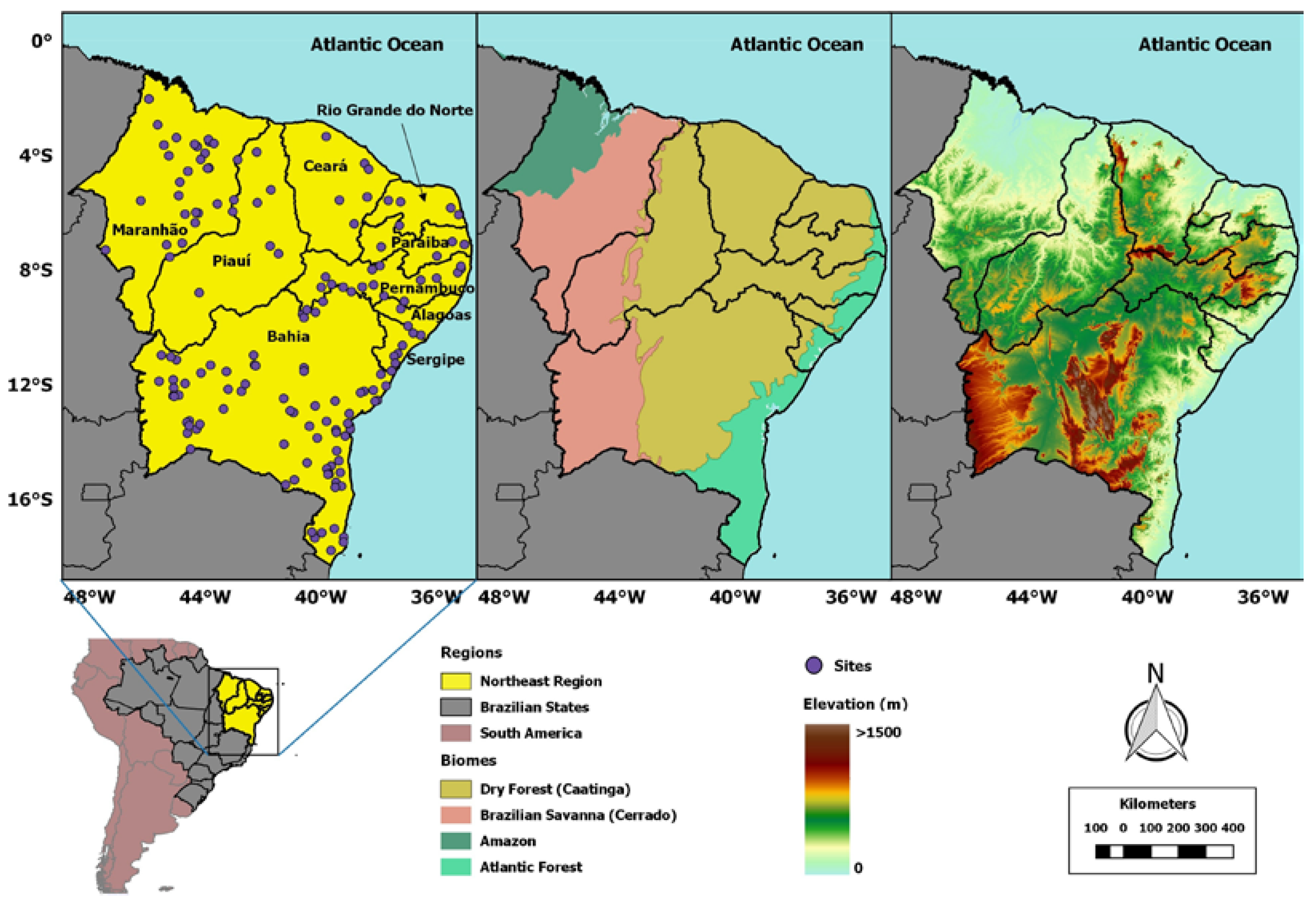
2.2. Study Area
2.3. Statistical Methods
2.3.1. Model
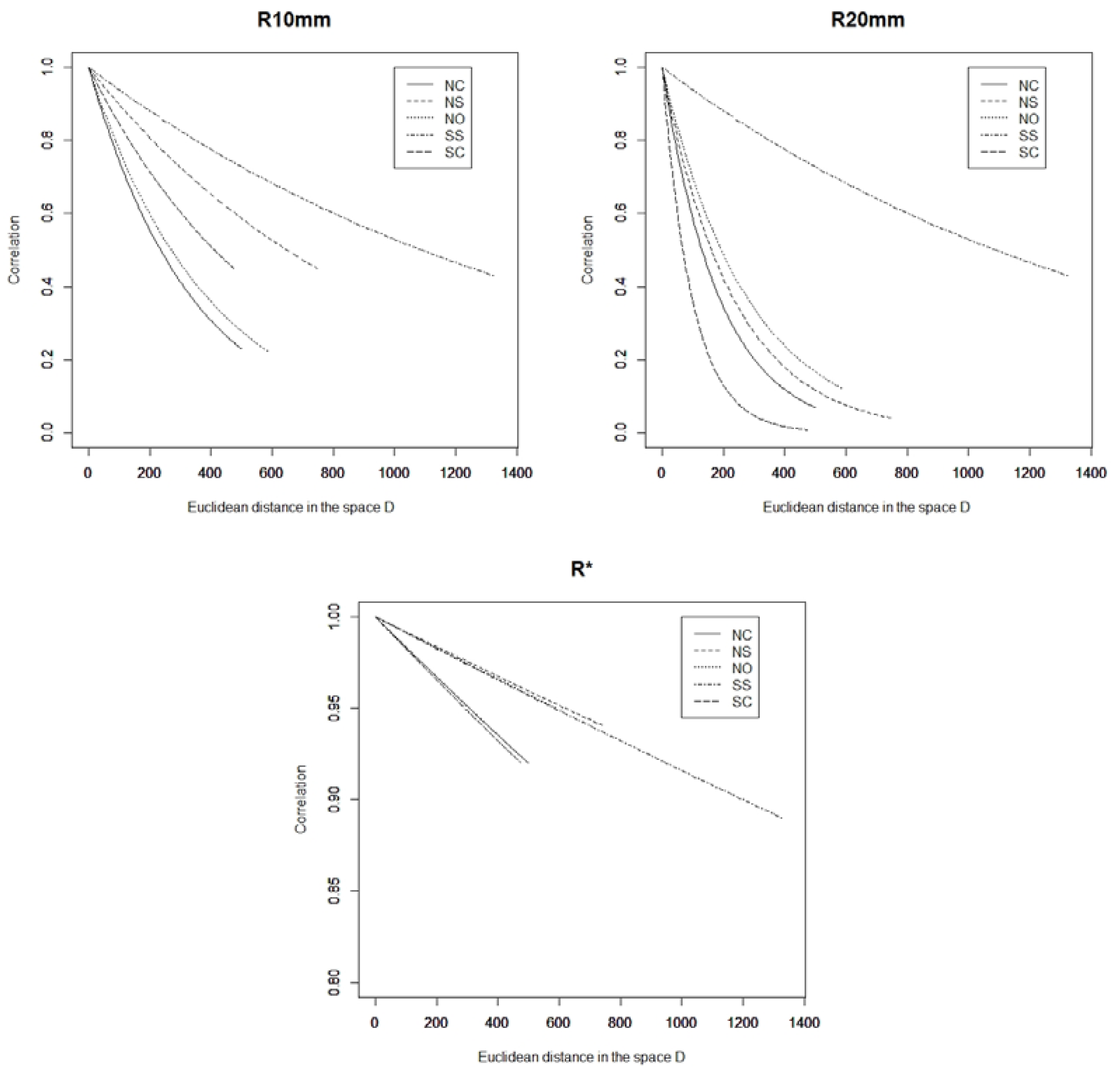
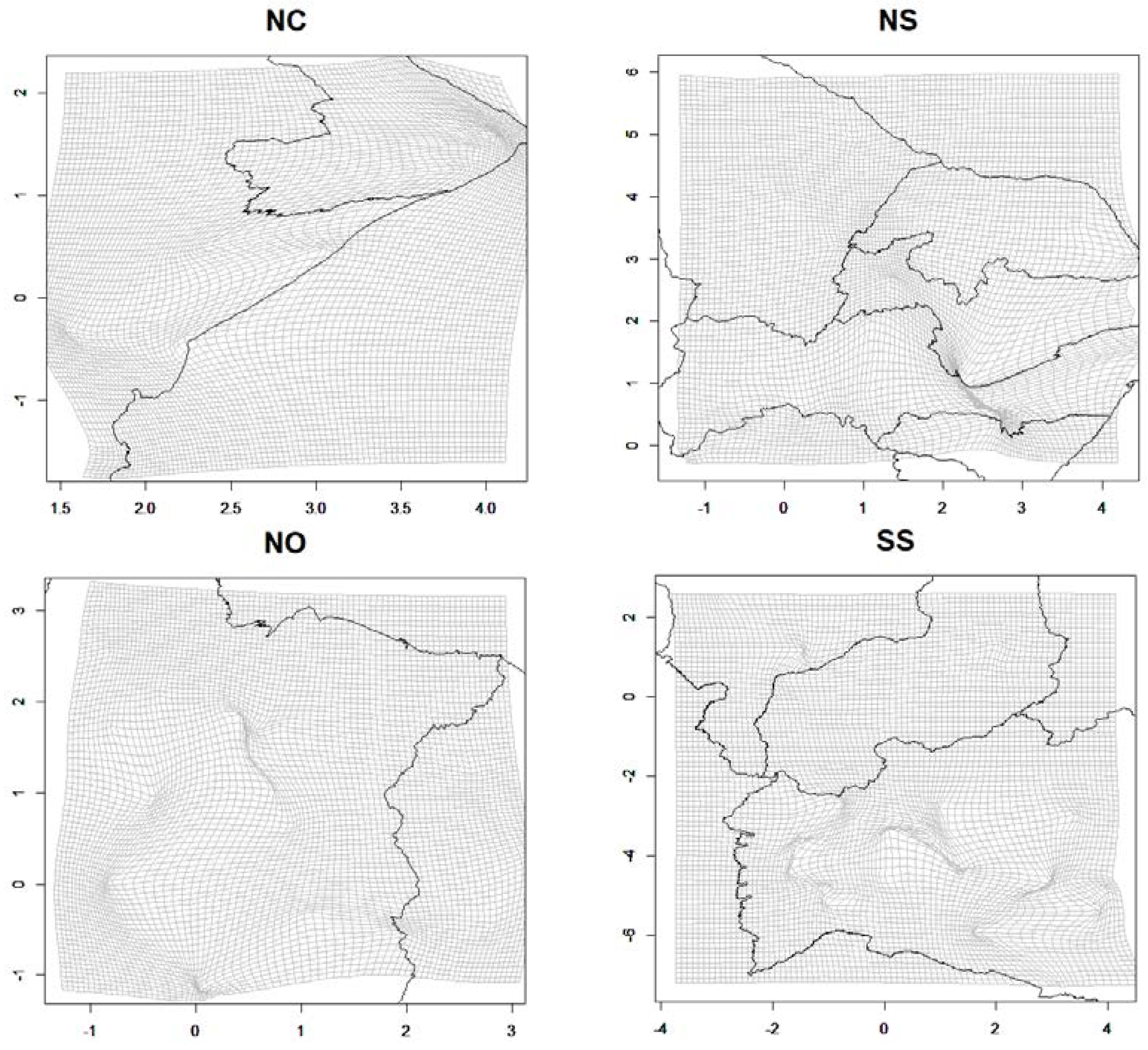
2.3.2. Spatial Component
2.3.3. Parameter Interpretation
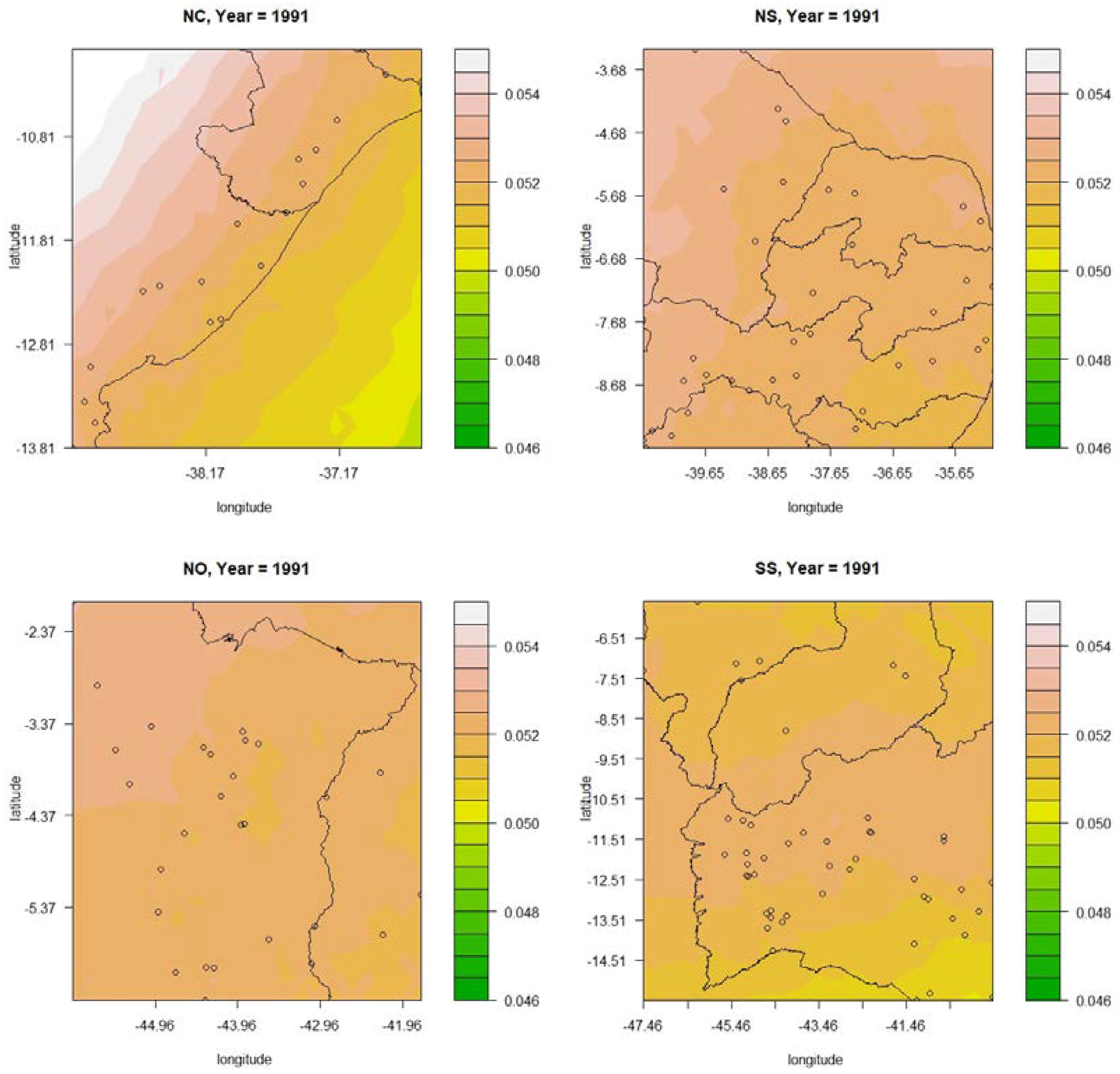
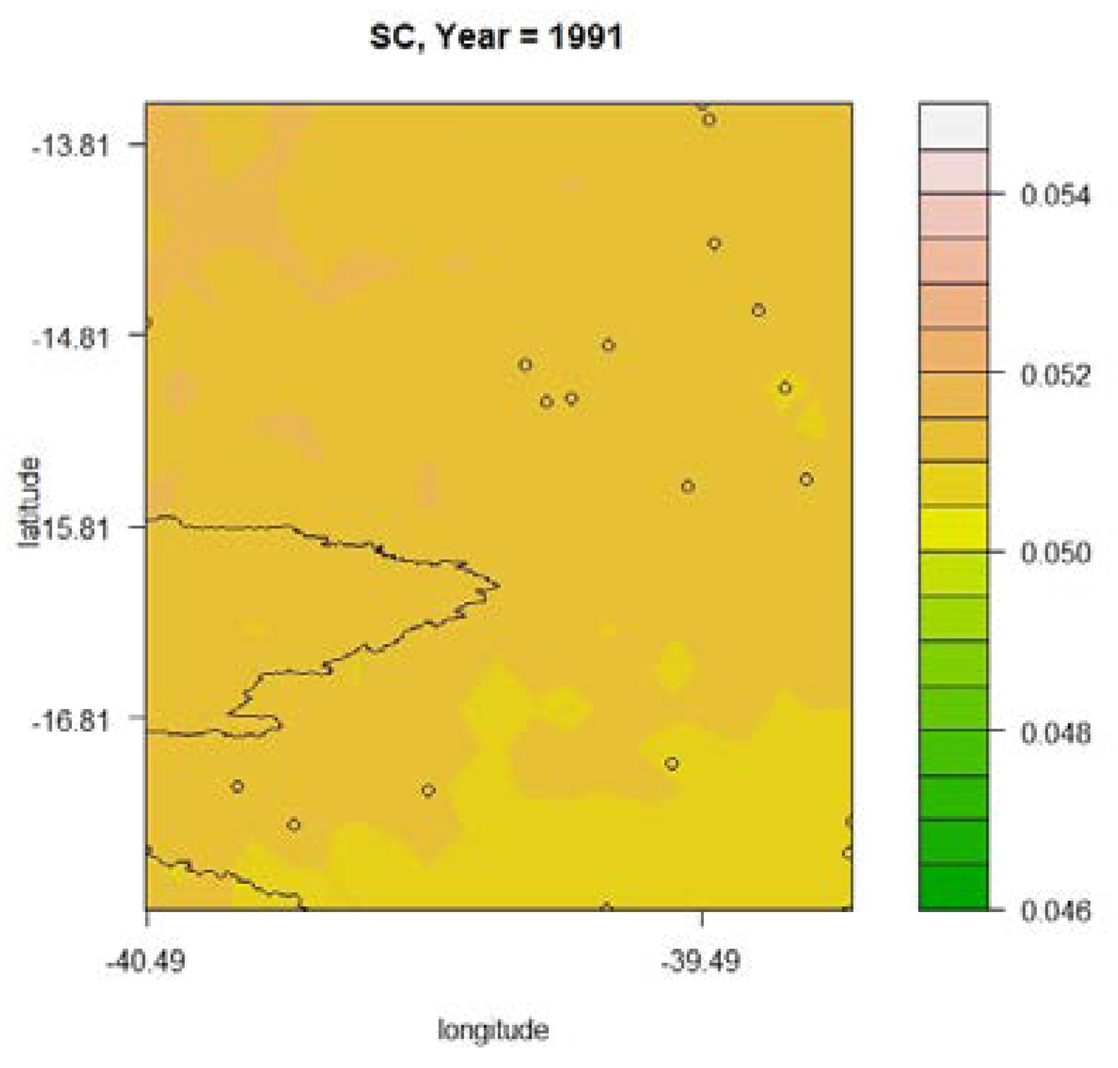
2.3.4. Spatial Interpolation of the R10 mm, R20 mm and R* Indices
3. Results and Discussion
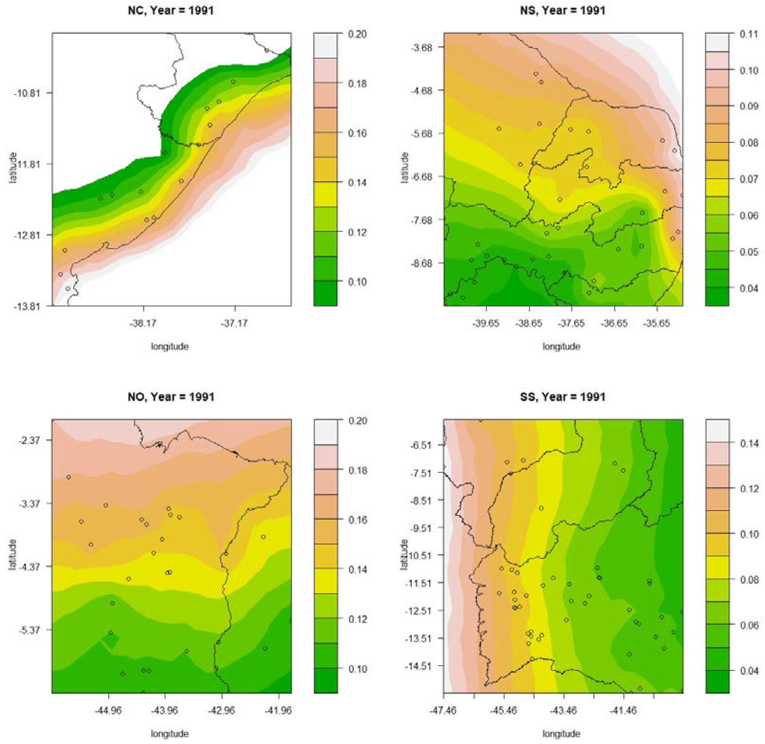
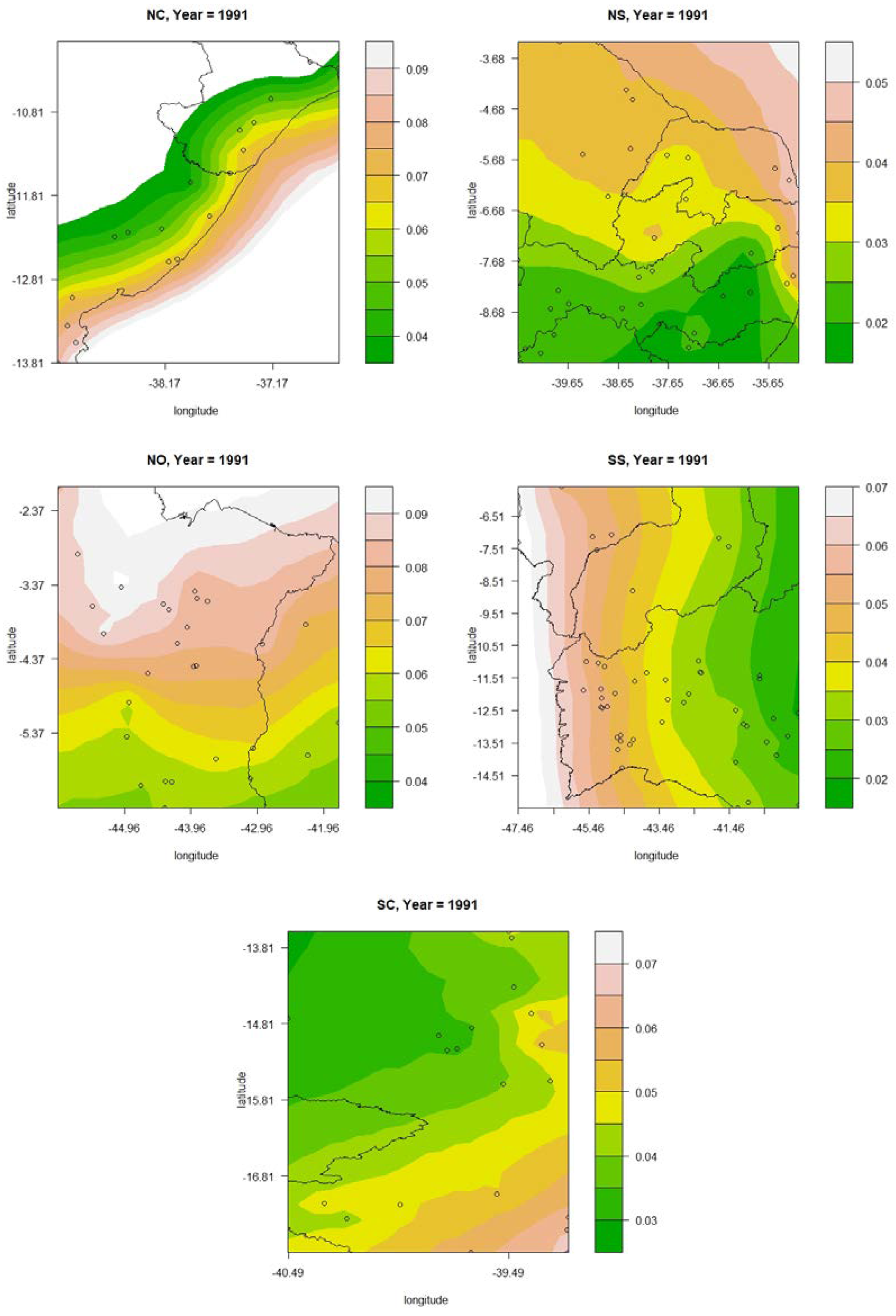
3.1. NC Subregion
3.1.1. Results Obtained for the R10 mm Index
3.1.2. Results Obtained for the R20 mm Index
3.1.3. Results Obtained for the R* mm Index
3.2. NS Subregion
3.2.1. Results Obtained for the R10 mm Index
3.2.2. Results Obtained for the R20 mm Index
3.2.3. Results Obtained for the R* mm Index
3.3. NO Subregion
3.3.1. Results Obtained for the R10 mm Index
3.3.2. Results Obtained for the R20 mm Index
3.3.3. Results Obtained for the R* Index
3.4. SS Subregion
3.4.1. Results Obtained for the R10 mm Index
3.4.2. Results Obtained for the R20 mm Index
3.4.3. Results Obtained for the R* Index
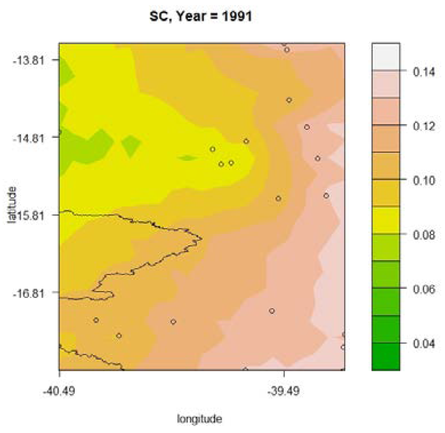
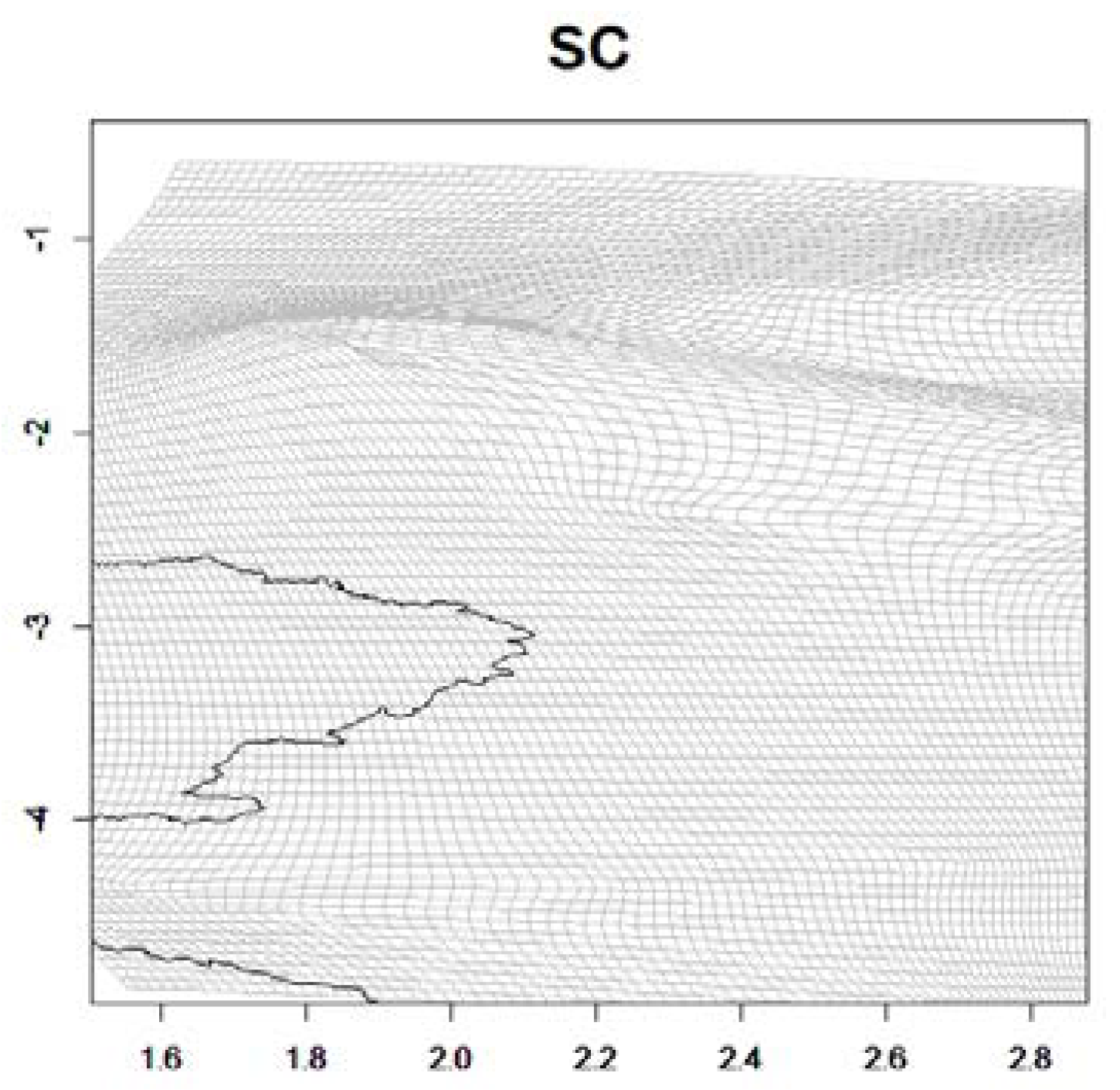
3.5. SC Subregion
3.5.1. Results Obtained for the R10 mm Index
3.5.2. Results Obtained for the R20 mm Index
3.5.3. Results Obtained for the R* Index
4. Conclusions
Supplementary Materials
Author Contributions
Funding
Institutional Review Board Statement
Informed Consent Statement
Data Availability Statement
Acknowledgments
Conflicts of Interest
References
- Krishnamurti, T.N.; Kishtawal, C.M.; LaRow, T.E.; Bachiochi, D.R.; Zhang, Z.; Williford, C.E.; Gadgil, S.; Surendran, S. Improved Weather and Seasonal Climate Forecasts from multimodel superensemble. Science 1999, 285, 1548–1550. [Google Scholar] [CrossRef] [Green Version]
- Grell, G.A.; Dévényi, D. A Generalized Approach to Parameterizing Convection Combining Ensemble and Data Assimilation Techniques. Geophys. Res. Lett. 2002, 29, 10–13. [Google Scholar] [CrossRef] [Green Version]
- Dantas, V.d.A.; Amorim, A.C.B.; Costa, M.d.S.; Santos e Silva, C.M. Downscaling Dinâmico Sobre o Nordeste Do Brasil Utilizando Um Modelo Climático Regional: Impacto de Diferentes Parametrizações Na Precipitação Simulada. Rev. Bras. Geogr. Física 2013, 6, 995–1008. [Google Scholar] [CrossRef] [Green Version]
- Yang, M.; Tan, Y.; Li, X.; Chen, X.; Zhang, C.; Yu, P. Influence of Cumulus Convection Schemes on Winter North Pacific Storm Tracks in the Regional Climate Model RegCM4.5. Int. J. Climatol. 2020, 40, 1294–1305. [Google Scholar] [CrossRef]
- Wang, Y.; Feng, J.; Luo, M.; Wang, J.; Qiu, Y. Uncertainties in Simulating Central Asia: Sensitivity to Physical Parameterizations Using Weather Research and Forecasting Model. Int. J. Climatol. 2020, 40, 5813–5828. [Google Scholar] [CrossRef]
- Zong, P.; Zhu, Y.; Tang, J. Sensitivity of Summer Precipitation in Regional Spectral Model Simulations over Eastern China to Physical Schemes: Daily, Extreme and Diurnal Cycle. Int. J. Climatol. 2019, 39, 4340–4357. [Google Scholar] [CrossRef]
- Rodrigues, D.T.; Gonçalves, W.A.; Spyrides, M.H.C.; Santos e Silva, C.M.; de Souza, D.O. Spatial Distribution of the Level of Return of Extreme Precipitation Events in Northeast Brazil. Int. J. Climatol. 2020, 40, 5098–5113. [Google Scholar] [CrossRef]
- Caldeira, T.L.; Beskow, S.; Mello, C.R.d.; Faria, L.C.; Souza, M.R.d.; Guedes, H.A.S. Modelagem Probabilística de Eventos de Precipitação Extrema No Estado Do Rio Grande Do Sul. Rev. Bras. Eng. Agrícola Ambient. 2015, 19, 197–203. [Google Scholar] [CrossRef] [Green Version]
- Quadros Gramosa, A.H.; Ferraz do Nascimento, F.; Castro Morales, F.E. A Bayesian Approach to Zero-Inflated Data in Extremes. Commun. Stat. Theory Methods 2020, 49, 4150–4161. [Google Scholar] [CrossRef]
- Gámiz-Fortis, S.R.; Esteban-Parra, M.J.; Trigo, R.M.; Castro-Díez, Y. Potential Predictability of an Iberian River Flow Based on Its Relationship with Previous Winter Global SST. J. Hydrol. 2010, 385, 143–149. [Google Scholar] [CrossRef]
- Paeth, H.; Girmes, R.; Menz, G.; Hense, A. Improving Seasonal Forecasting in the Low Latitudes. Mon. Weather Rev. 2006, 134, 1859–1879. [Google Scholar] [CrossRef]
- Asadieh, B.; Krakauer, N.Y. Global Trends in Extreme Precipitation: Climate Models versus Observations. Hydrol. Earth Syst. Sci. 2015, 19, 877–891. [Google Scholar] [CrossRef] [Green Version]
- Du, H.; Alexander, L.V.; Donat, M.G.; Lippmann, T.; Srivastava, A.; Salinger, J.; Kruger, A.; Choi, G.; He, H.S.; Fujibe, F.; et al. Precipitation from Persistent Extremes Is Increasing in Most Regions and Globally. Geophys. Res. Lett. 2019, 46, 6041–6049. [Google Scholar] [CrossRef] [Green Version]
- Sun, X.; Renard, B.; Thyer, M.; Westra, S.; Lang, M. A Global Analysis of the Asymmetric Effect of ENSO on Extreme Precipitation. J. Hydrol. 2015, 530, 51–65. [Google Scholar] [CrossRef] [Green Version]
- Michaels, P.J.; Knappenberger, P.C.; Frauenfeld, O.W.; Davis, R.E. Trends in Precipitation on the Wettest Days of the Year across the Contiguous USA. Int. J. Climatol. 2004, 24, 1873–1882. [Google Scholar] [CrossRef]
- Bartels, R.J.; Black, A.W.; Keim, B.D. Trends in Precipitation Days in the United States. Int. J. Climatol. 2020, 40, 1038–1048. [Google Scholar] [CrossRef]
- Palharini, R.; Vila, D.; Rodrigues, D.; Palharini, R.; Mattos, E.; Undurraga, E. Analysis of Extreme Rainfall and Natural Disasters Events Using Satellite Precipitation Products in Different Regions of Brazil. Atmosphere 2022, 13, 1680. [Google Scholar] [CrossRef]
- Santos, E.B.; Lucio, P.S.; Santos e Silva, C.M. Seasonal Analysis of Return Periods for Maximum Daily Precipitation in the Brazilian Amazon. J. Hydrometeorol. 2015, 16, 973–984. [Google Scholar] [CrossRef]
- Rodrigues, D.T.; Gonçalves, W.A.; Spyrides, M.H.C.; Santos e Silva, C.M. Spatial and Temporal Assessment of the Extreme and Daily Precipitation of the Tropical Rainfall Measuring Mission Satellite in Northeast Brazil. Int. J. Remote Sens. 2019, 41, 549–572. [Google Scholar] [CrossRef]
- da Cunha Luz Barcellos, P.; Cataldi, M. Flash Flood and Extreme Rainfall Forecast through One-Way Coupling of WRF-SMAP Models: Natural Hazards in Rio de Janeiro State. Atmosphere 2020, 11, 834. [Google Scholar] [CrossRef]
- Oliveira, P.T.; Santos e Silva, C.M.; Lima, K.C. Climatology and Trend Analysis of Extreme Precipitation in Subregions of Northeast Brazil. Theor. Appl. Climatol. 2017, 130, 77–90. [Google Scholar] [CrossRef]
- Morales, F.E.C.; Rodrigues, D.T. Spatiotemporal Nonhomogeneous Poisson Model with a Seasonal Component Applied to the Analysis of Extreme Rainfall. J. Appl. Stat. 2022. [Google Scholar] [CrossRef]
- McLeod, J.; Shepherd, M.; Konrad, C.E. Spatio-Temporal Rainfall Patterns around Atlanta, Georgia and Possible Relationships to Urban Land Cover. Urban Clim. 2017, 21, 27–42. [Google Scholar] [CrossRef]
- Kirshen, P.; Aytur, S.; Hecht, J.; Walker, A.; Burdick, D.; Jones, S.; Fennessey, N.; Bourdeau, R.; Mather, L. Integrated Urban Water Management Applied to Adaptation to Climate Change. Urban Clim. 2018, 24, 247–263. [Google Scholar] [CrossRef]
- Gidhagen, L.; Olsson, J.; Amorim, J.H.; Asker, C.; Belusic, D.; Carvalho, A.C.; Engardt, M.; Hundecha, Y.; Körnich, H.; Lind, P.; et al. Towards Climate Services for European Cities: Lessons Learnt from the Copernicus Project Urban SIS. Urban Clim. 2020, 31, 100549. [Google Scholar] [CrossRef]
- Rodrigues, D.T.; Gonçalves, W.A.; Spyrides, M.H.; Andrade, L.D.; de Souza, D.O.; de Araujo, P.A.; da Silva, A.C.; e Silva, C.M. Probability of Occurrence of Extreme Precipitation Events and Natural Disasters in the City of Natal, Brazil. Urban Clim. 2021, 35, 100753. [Google Scholar] [CrossRef]
- Bezerra, B.G.; Silva, L.L.; Santos e Silva, C.M.; de Carvalho, G.G. Changes of Precipitation Extremes Indices in São Francisco River Basin, Brazil from 1947 to 2012. Theor. Appl. Climatol. 2019, 135, 565–576. [Google Scholar] [CrossRef]
- Marengo, J.A.; Valverde, M.C.; Obregon, G.O. Observed and Projected Changes in Rainfall Extremes in the Metropolitan Area of São Paulo. Clim. Res. 2013, 57, 61–72. [Google Scholar] [CrossRef] [Green Version]
- Marengo, J.A.; Torres, R.R.; Alves, L.M. Drought in Northeast Brazil—Past, Present, and Future. Theor. Appl. Climatol. 2017, 129, 1189–1200. [Google Scholar] [CrossRef]
- Da Silva, P.E.; Santos e Silva, C.M.; Spyrides, M.H.C.; Andrade, L.d.M.B. Precipitation and Air Temperature Extremes in the Amazon and Northeast Brazil. Int. J. Climatol. 2019, 39, 579–595. [Google Scholar] [CrossRef]
- Araujo Palharini, R.S.; Vila, D.A.; Rodrigues, D.T.; Palharini, R.C.; Mattos, E.V.; Pedra, G.U. Assessment of Extreme Rainfall Estimates from Satellite-Based: Regional Analysis. Remote Sens. Appl. Soc. Environ. 2021, 23, 100603. [Google Scholar] [CrossRef]
- Enfield, D.B. Relationships of Inter-American Rainfall to Tropical Atlantic and Pacific SST Variability. Geophys. Res. Lett. 1996, 23, 3305–3308. [Google Scholar] [CrossRef]
- Seth, A.; Rauscher, S.A.; Camargo, S.J.; Qian, J.H.; Pal, J.S. RegCM3 Regional Climatologies for South America Using Reanalysis and ECHAM Global Model Driving Fields. Clim. Dyn. 2007, 28, 461–480. [Google Scholar] [CrossRef] [Green Version]
- Nobre, P.; Marengo, J.A.; Cavalcanti, I.F.A.; Obregon, G.; Barros, V.; Camilloni, I.; Campos, N.; Ferreira, A.G. Seasonal-to-Decadal Predictability and Prediction of South American Climate. J. Clim. 2006, 19, 5988–6004. [Google Scholar] [CrossRef] [Green Version]
- Misra, V.; Zhang, Y. The Fidelity of NCEP CFS Seasonal Hindcasts over Nordeste. Mon. Weather Rev. 2007, 135, 618–627. [Google Scholar] [CrossRef]
- Hounsou-Gbo, G.A.; Araujo, M.; Bourlès, B.; Veleda, D.; Servain, J. Tropical Atlantic Contributions to Strong Rainfall Variability along the Northeast Brazilian Coast. Adv. Meteorol. 2015, 2015, 902084. [Google Scholar] [CrossRef] [Green Version]
- Duarte, J.L.; Diaz-Quijano, F.A.; Batista, A.C.; Giatti, L.L. Climatic Variables Associated with Dengue Incidence in a City of the Western Brazilian Amazon Region. Rev. Soc. Bras. Med. Trop. 2019, 52, 1–8. [Google Scholar] [CrossRef] [Green Version]
- De Oliveira, P.T.; Silva, C.M.S.E.; Lima, K.C. Linear Trend of Occurrence and Intensity of Heavy Rainfall Events on Northeast Brazil. Atmos. Sci. Lett. 2014, 15, 172–177. [Google Scholar] [CrossRef]
- Grimm, A.M.; Tedeschi, R.G. ENSO and Extreme Rainfall Events in South America. J. Clim. 2009, 22, 1589–1609. [Google Scholar] [CrossRef]
- Min, S.K.; Zhang, X.; Zwiers, F.W.; Hegerl, G.C. Human Contribution to More-Intense Precipitation Extremes. Nature 2011, 470, 378–381. [Google Scholar] [CrossRef] [PubMed]
- Donat, M.G.; Lowry, A.L.; Alexander, L.V.; O’Gorman, P.A.; Maher, N. More Extreme Precipitation in the Worldâ €TM s Dry and Wet Regions. Nat. Clim. Chang. 2016, 6, 508–513. [Google Scholar] [CrossRef]
- Huntington, T.G. Evidence for Intensification of the Global Water Cycle: Review and Synthesis. J. Hydrol. 2006, 319, 83–95. [Google Scholar] [CrossRef]
- Trenberth, K.E. Changes in Precipitation with Climate Change. Clim. Res. 2011, 47, 123–138. [Google Scholar] [CrossRef] [Green Version]
- IPCC. Climate Change 2021 The Physical Science Basis WGI; IPCC: Geneva, Switzerland, 2021; Volume 34, ISBN 9781009157896. [Google Scholar]
- IPCC. IPCC Part A: Global and Sectoral Aspects. (Contribution of Working Group II to the Fifth Assessment Report of the Intergovernmental Panel on Climate Change; Climate Change 2014: Impacts, Adaptation, and Vulnerability; IPCC: Geneva, Switzerland, 2014; p. 1132. [Google Scholar]
- Aumann, H.H.; Behrangi, A.; Wang, Y. Increased Frequency of Extreme Tropical Deep Convection: AIRS Observations and Climate Model Predictions. Geophys. Res. Lett. 2018, 45, 13530–13537. [Google Scholar] [CrossRef] [Green Version]
- Serrano-Notivoli, R.; Beguería, S.; Saz, M.Á.; de Luis, M. Recent Trends Reveal Decreasing Intensity of Daily Precipitation in Spain. Int. J. Climatol. 2018, 38, 4211–4224. [Google Scholar] [CrossRef]
- Santos, M.; Fonseca, A.; Fragoso, M.; Santos, J.A. Recent and Future Changes of Precipitation Extremes in Mainland Portugal. Theor. Appl. Climatol. 2019, 137, 1305–1319. [Google Scholar] [CrossRef]
- Zeder, J.; Fischer, E.M. Observed Extreme Precipitation Trends and Scaling in Central Europe. Weather Clim. Extrem. 2020, 29, 100266. [Google Scholar] [CrossRef]
- Zhang, M.; Chen, Y.; Shen, Y.; Li, B. Tracking Climate Change in Central Asia through Temperature and Precipitation Extremes. J. Geogr. Sci. 2019, 29, 3–28. [Google Scholar] [CrossRef] [Green Version]
- Saddique, N.; Khaliq, A.; Bernhofer, C. Trends in Temperature and Precipitation Extremes in Historical (1961–1990) and Projected (2061–2090) Periods in a Data Scarce Mountain Basin, Northern Pakistan. Stoch. Environ. Res. Risk Assess. 2020, 34, 1441–1455. [Google Scholar] [CrossRef]
- Harrison, L.; Funk, C.; Peterson, P. Identifying Changing Precipitation Extremes in Sub-Saharan Africa with Gauge and Satellite Products. Environ. Res. Lett. 2019, 14, 085007. [Google Scholar] [CrossRef]
- Gebrechorkos, S.H.; Hülsmann, S.; Bernhofer, C. Changes in Temperature and Precipitation Extremes in Ethiopia, Kenya, and Tanzania. Int. J. Climatol. 2019, 39, 18–30. [Google Scholar] [CrossRef] [Green Version]
- da Silva, R.M.; Santos, C.A.G.; da Costa Silva, J.F.C.B.; Silva, A.M.; Brasil Neto, R.M. Spatial Distribution and Estimation of Rainfall Trends and Erosivity in the Epitácio Pessoa Reservoir Catchment, Paraíba, Brazil. Nat. Hazards 2020, 102, 829–849. [Google Scholar] [CrossRef]
- Rodrigues, D.T.; Santos e Silva, C.M.; Dos Reis, J.S.; Palharini, R.S.A.; Cabral Júnior, J.B.; da Silva, H.J.F.; Mutti, P.R.; Bezerra, B.G.; Gonçalves, W.A. Evaluation of the Integrated Multi-Satellite Retrievals for the Global Precipitation Measurement (Imerg) Product in the São Francisco Basin (Brazil). Water 2021, 13, 2714. [Google Scholar] [CrossRef]
- Silva, J.D.S.; Cabral Júnior, J.B.; Rodrigues, D.T.; Silva, F.D.D.S. Climatology and Significant Trends in Air Temperature in Alagoas, Northeast Brazil. Theor. Appl. Climatol. 2023, 151, 1805–1824. [Google Scholar] [CrossRef]
- Wanhe, L.; Wenxiang, C. Temporal Trends Features in Consecutive Days of Extreme Precipitation over China, 1951–2017. Mausam 2019, 70, 321–328. [Google Scholar] [CrossRef]
- Wang, W.; Tang, H.; Li, J.; Hou, Y. Spatial-Temporal Variations of Extreme Precipitation Characteristics and Its Correlation with El Niño-Southern Oscillation during 1960–2019 in Hubei Province, China. Atmosphere 2022, 13, 1922. [Google Scholar] [CrossRef]
- Xia, Y.; Dan, D.; Liu, H.; Zhou, H.; Wan, Z. Spatiotemporal Distribution of Precipitation over the Mongolian Plateau during 1976–2017. Atmosphere 2022, 13, 2132. [Google Scholar] [CrossRef]
- Zechie, P.R.; Chiao, S. Climate Variability of Atmospheric Rivers and Droughts over the West Coast of the United States from 2006 to 2019. Atmosphere 2021, 12, 201. [Google Scholar] [CrossRef]
- Brazel, A. June Temperature Trends in the Southwest Deserts of the USA (1950–2018) and Implications for Our Urban Areas. Atmosphere 2019, 10, 800. [Google Scholar] [CrossRef] [Green Version]
- Dunn, R.J.H.; Alexander, L.V.; Donat, M.G.; Zhang, X.; Bador, M.; Herold, N.; Lippmann, T.; Allan, R.; Aguilar, E.; Barry, A.A.; et al. Development of an Updated Global Land In Situ-Based Data Set of Temperature and Precipitation Extremes: HadEX3. J. Geophys. Res. Atmos. 2020, 125, e2019JD032263. [Google Scholar] [CrossRef]
- Sillmann, J.; Thorarinsdottir, T.; Keenlyside, N.; Schaller, N.; Alexander, L.V.; Hegerl, G.; Seneviratne, S.I.; Vautard, R.; Zhang, X.; Zwiers, F.W. Understanding, Modeling and Predicting Weather and Climate Extremes: Challenges and Opportunities. Weather Clim. Extrem. 2017, 18, 65–74. [Google Scholar] [CrossRef]
- Morales, F.E.C.; Vicini, L.; Hotta, L.K.; Achcar, J.A. A Nonhomogeneous Poisson Process Geostatistical Model. Stoch. Environ. Res. Risk Assess. 2017, 31, 493–507. [Google Scholar] [CrossRef]
- Campion, W.M.; Rubin, D.B. Multiple Imputation for Nonresponse in Surveys; John Wiley & Sons, Inc.: Hoboken, NJ, USA, 1989; Volume 26, ISBN 047108705X. [Google Scholar]
- Honaker, J.; King, G.; Blackwell, M. Amelia II: A Program for Missing Data, R Package Version 1.5., 2012. J. Stat. Softw. 2011, 45, 1–3. [Google Scholar]
- IBGE Instituto Brasileiro de Geografia e Estatística (IBGE). Estimativas Da População Residente No Brasil e Unidades Da Federação Com Data de Referência Em 1o de Julho de 2021. Inst. Bras. Geogr. Estat. 2021, 1–119. [Google Scholar]
- de Abreu, L.P.; Gonçalves, W.A.; Mattos, E.V.; Mutti, P.R.; Rodrigues, D.T.; da Silva, M.P.A. Clouds’ Microphysical Properties and Their Relationship with Lightning Activity in Northeast Brazil. Remote Sens. 2021, 13, 4491. [Google Scholar] [CrossRef]
- Calderari, E.B.; Gomes, C.P.; Beatrice, F.D.O.; Torres, R.L. As Contribuições Da Nova Sudene Para o Desenvolvimento Do Nordeste. Rev. Grifos 2019, 29, 11. [Google Scholar] [CrossRef]
- Rao, V.B.; Franchito, S.H.; Santo, C.M.E.; Gan, M.A. An Update on the Rainfall Characteristics of Brazil: Seasonal Variations and Trends in 1979–2011. Int. J. Climatol. 2016, 36, 291–302. [Google Scholar] [CrossRef]
- Chaves, R.R.; Cavalcanti, I.F.A. Atmospheric Circulation Features Associated with Rainfall Variability over Southern Northeast Brazil. Mon. Weather Rev. 2001, 129, 2614–2626. [Google Scholar] [CrossRef]
- Carvalho, L.M.V.; Jones, C.; Liebmann, B. The South Atlantic Convergence Zone: Intensity, Form, Persistence, and Relationships with Intraseasonal to Interannual Activity and Extreme Rainfall. J. Clim. 2004, 17, 88–108. [Google Scholar] [CrossRef]
- Nobre, P.; Shukla, J. Variations of Sea Surface Temperature, Wind Stress, and Rainfall over the Tropical Atlantic and South America. J. Clim. 1996, 9, 2464–2479. [Google Scholar] [CrossRef]
- Boers, N.; Bookhagen, B.; Marwan, N.; Kurths, J.; Marengo, J. Complex Networks Identify Spatial Patterns of Extreme Rainfall Events of the South American Monsoon System. Geophys. Res. Lett. 2013, 40, 4386–4392. [Google Scholar] [CrossRef] [Green Version]
- Figueroa, S.N.; Bonatti, J.P.; Kubota, P.Y.; Grell, G.A.; Morrison, H.; Barros, S.R.M.; Fernandez, J.P.R.; Ramirez, E.; Siqueira, L.; Luzia, G.; et al. The Brazilian Global Atmospheric Model (BAM): Performance for Tropical Rainfall Forecasting and Sensitivity to Convective Scheme and Horizontal Resolution. Weather Forecast. 2016, 31, 1547–1572. [Google Scholar] [CrossRef]
- Lucena, R.L.; Borges Da Silva, F.E.; De Medeiros Aprígio, T.R.; Bezerra Cabral Júnior, J. The Influence of Altitude on the Climate of Semiarid Areas: Contributions to Conservation. Int. J. Clim. Chang. Impacts Responses 2022, 14, 81–93. [Google Scholar] [CrossRef]
- Lyra, G.B.; Oliveira-Júnior, J.F.; Zeri, M. Cluster Analysis Applied to the Spatial and Temporal Variability of Monthly Rainfall in Alagoas State, Northeast of Brazil. Int. J. Climatol. 2014, 34, 3546–3558. [Google Scholar] [CrossRef]
- Barbieri, A.F.; Guedes, G.R.; Noronha, K.; Queiroz, B.L.; Domingues, E.P.; Rigotti, J.I.R.; da Motta, G.P.; Chein, F.; Cortezzi, F.; Confalonieri, U.E.; et al. Population Transitions and Temperature Change in Minas Gerais, Brazil: A Multidimensional Approach. Rev. Bras. Estud. Popul. 2015, 32, 461–488. [Google Scholar] [CrossRef] [Green Version]
- Macedo, M.J.H.; de Souza Guedes, R.V.; de Sousa, F.D.A.S.; da Cunha Dantas, F.R. Análise Do Índice Padronizado de Precipitação Para o Estado Da Paraíba, Brasil. Rev. Ambient. Agua 2014, 9, 445–458. [Google Scholar] [CrossRef]
- Zanella, M.E. Análise Multitemporal Dos Desastres Naturais Hidroclimatológicos Do Estado Do Ceará: Contribuições Das Geotecnologias à Gestão Dos Riscos Naturais. Rev. Geonorte 2012, 1, 907–920. [Google Scholar]
- Morales, F.E.C.; Vicini, L. A Non-Homogeneous Poisson Process Geostatistical Model with Spatial Deformation. AStA Adv. Stat. Anal. 2020, 104, 503–527. [Google Scholar] [CrossRef]
- Goel, A.L. A Guidebook for Software Reliability Assessment; Syracuse University: Syracuse, NY, USA, 1983. [Google Scholar]
- Sampson, P.D.; Guttorp, P. Estimation of Nonstationary Nonparametric Spatial Covariance Structure. J. Am. Stat. Assoc. 2014, 87, 108–119. [Google Scholar] [CrossRef]
- Gomes, H.B.; Ambrizzi, T.; Pontes da Silva, B.F.; Hodges, K.; Silva Dias, P.L.; Herdies, D.L.; Silva, M.C.L.; Gomes, H.B. Climatology of Easterly Wave Disturbances over the Tropical South Atlantic. Clim. Dyn. 2019, 53, 1393–1411. [Google Scholar] [CrossRef] [Green Version]
- Kousky, V.E. Frontal Influences on Northeast Brazil. Mon. Weather Rev. 1979, 107, 1140–1153. [Google Scholar] [CrossRef]
- Zhou, J.; Lau, K.M. Principal Modes of Interannual and Decadal Variability of Summer Rainfall over South America. Int. J. Climatol. 2001, 21, 1623–1644. [Google Scholar] [CrossRef]
- Reboita, M.S.; Rodrigues, M.; Silva, L.F.; Alves, M.A. Aspectos Climáticos Do Estado de Minas Gerais. Rev. Bras. Climatol. 2015, 17, 206–226. [Google Scholar]
- Palharini, R.S.A.; Vila, D.A.; Rodrigues, D.T.; Quispe, D.P.; Palharini, R.C.; de Siqueira, R.A.; de Sousa Afonso, J.M. Assessment of the Extreme Precipitation by Satellite Estimates over South America. Remote Sens. 2020, 12, 2085. [Google Scholar] [CrossRef]
- Araújo Palharini, R.S.; Vila, D.A. Climatological Behavior of Precipitating Clouds in the Northeast Region of Brazil. Adv. Meteorol. 2017, 2017, 5916150. [Google Scholar] [CrossRef] [Green Version]
- Reis, L.; Silva, C.M.S.E.; Bezerra, B.; Mutti, P.; Spyrides, M.H.; Silva, P.; Magalhães, T.; Ferreira, R.; Rodrigues, D.; Andrade, L. Influence of Climate Variability on Soybean Yield in Matopiba, Brazil. Atmosphere 2020, 11, 1130. [Google Scholar] [CrossRef]


| Subregion | Parameter | Mean | 50% | 2.5% | 97.5% |
|---|---|---|---|---|---|
| NC | 6.42 × 10⁻⁶ | 6.38 × 10⁻⁶ | 5.86 × 10⁻⁶ | 7.11 × 10⁻⁶ | |
| 1.04 | 1.04 | 1.03 | 1.05 | ||
| 0.33 | 0.13 | 0.01 | 1.18 | ||
| 14.93 | 14.81 | 4.63 | 26.44 | ||
| 0.30 | 0.30 | −0.04 | 0.66 | ||
| −0.49 | 0.50 | −0.78 | −0.19 | ||
| NS | 1.42 × 10⁻⁵ | 1.41 × 10⁻⁵ | 1.24 × 10⁻⁵ | 1.61 × 10⁻⁵ | |
| 1.01 | 1.01 | 1.00 | 1.03 | ||
| 0.26 | 0.12 | 0.01 | 0.96 | ||
| 10.39 | 10.38 | 6.77 | 14.20 | ||
| 0.04 | 0.04 | −.05 | 0.13 | ||
| 0.10 | 0.10 | 0.02 | 0.19 | ||
| NO | 8.08 × 10⁻⁶ | 8.09 × 10⁻⁶ | 7.23 × 10⁻⁶ | 8.77 × 10⁻⁶ | |
| 1.02 | 1.02 | 1.01 | 1.03 | ||
| 0.29 | 0.16 | 0.01 | 0.96 | ||
| 8.74 | 8.78 | 5.62 | 11.55 | ||
| −0.03 | −0.03 | −0.09 | 0.03 | ||
| 0.13 | 0.13 | 0.60 | 0.20 | ||
| SS | 9.22 × 10⁻⁶ | 9.18 × 10⁻⁶ | 8.38 × 10⁻⁶ | 1.03 × 10⁻⁵ | |
| 1.00 | 1.00 | 0.99 | 1.01 | ||
| 0.07 | 0.04 | 0.01 | 0.33 | ||
| 1.75 | 1.67 | 0.00 | 3.74 | ||
| −0.17 | −0.17 | −0.20 | −0.13 | ||
| 0.00 | 0.00 | −0.03 | 0.04 | ||
| SC | 1.28 × 10⁻⁵ | 1.27 × 10⁻⁵ | 1.15 × 10⁻⁵ | 1.41 × 10⁻⁵ | |
| 1.00 | 1.00 | 0.98 | 1.01 | ||
| 0.19 | 0.07 | 0.01 | 0.75 | ||
| 16.74 | 17.00 | 6.15 | 26.84 | ||
| 0.20 | 0.20 | −0.06 | 0.44 | ||
| −0.03 | −0.02 | −0.20 | 0.11 |
| Subregion | Parameter | Mean | 50% | 2.5% | 97.5% |
|---|---|---|---|---|---|
| NC | 7.25 × 10⁻⁶ | 7.23 × 10⁻⁶ | 5.93 × 10⁻⁶ | 8.73 × 10⁻⁶ | |
| 1.03 | 1.03 | 1.01 | 1.05 | ||
| 0.6 | 0.19 | 0.01 | 2.12 | ||
| 16.84 | 17.04 | 4.20 | 28.80 | ||
| 0.40 | 0.41 | 0.00 | 0.81 | ||
| −0.59 | −0.60 | −0.92 | −0.22 | ||
| NS | 8.27 × 10⁻⁶ | 8.17 × 10⁻⁶ | 6.99 × 10⁻⁶ | 1.02 × 10⁻⁵ | |
| 1.01 | 1.01 | 0.99 | 1.03 | ||
| 0.25 | 0.13 | 0.01 | 0.84 | ||
| 9.43 | 9.55 | 3.36 | 14.54 | ||
| 0.02 | 0.02 | −0.12 | 0.15 | ||
| 0.08 | 0.08 | −0.02 | 0.19 | ||
| NO | 9.82 × 10⁻⁶ | 9.72 × 10⁻⁶ | 8.61 × 10⁻⁶ | 1.15 × 10⁻⁵ | |
| 1.02 | 1.02 | 1.01 | 1.04 | ||
| 0.40 | 0.17 | 0.01 | 1.29 | ||
| 8.04 | 7.98 | 4.58 | 11.66 | ||
| −0.03 | −0.03 | −0.10 | 0.06 | ||
| 0.11 | 0.11 | 0.02 | 0.20 | ||
| SS | 1.65 × 10⁻⁵ | 1.65 × 10⁻⁵ | 1.42 × 10⁻⁵ | 1.87 × 10⁻⁵ | |
| 0.98 | 0.98 | 0.97 | 0.99 | ||
| 0.06 | 0.03 | 0.01 | 0.22 | ||
| 0.27 | 0.27 | −1.86 | 2.37 | ||
| −0.18 | −0.18 | −0.22 | −0.13 | ||
| 0.01 | 0.01 | −0.04 | 0.05 | ||
| SC | 1.20 × 10⁻⁵ | 1.19 × 10⁻⁵ | 9.57 × 10⁻⁶ | 1.46 × 10⁻⁵ | |
| 0.97 | 097 | 0.95 | 0.99 | ||
| 1.13 | 0.25 | 0.01 | 4.92 | ||
| 15.25 | 15.45 | 5.72 | 25.48 | ||
| 0.22 | 0.23 | −0.02 | 0.47 | ||
| −0.13 | −0.13 | −0.27 | 0.01 |
| Subregion | Parameter | Mean | 50% | 2.5% | 97.5% |
|---|---|---|---|---|---|
| NC | 1.03 × 10⁻⁵ | 1.03 × 10⁻⁵ | 8.31 × 10⁻⁶ | 0.21 × 10⁻⁵ | |
| 1.07 | 1.07 | 1.06 | 1.10 | ||
| 0.02 | 0.01 | 0.01 | 0.05 | ||
| 7.16 | 6.94 | 4.19 | 11.33 | ||
| −0.02 | −0.03 | −0.12 | 0.12 | ||
| 0.01 | 0.02 | −0.08 | 0.08 | ||
| NS | 1.44 × 10⁻⁵ | 1.42 × 10⁻⁵ | 1.28 × 10⁻⁵ | 1.62 × 10⁻⁵ | |
| 1.05 | 1.05 | 1.04 | 1.07 | ||
| 0.01 | 0.01 | 0.01 | 0.03 | ||
| 7.78 | 7.76 | 7.11 | 8.59 | ||
| 0.00 | 0.00 | −0.02 | 0.02 | ||
| 0.01 | 0.01 | 0.00 | 0.02 | ||
| NO | 1.36 × 10⁻⁵ | 1.37 × 10⁻⁵ | 1.15 × 10⁻⁵ | 1.54 × 10⁻⁵ | |
| 1.06 | 1.06 | 1.05 | 1.08 | ||
| 0.01 | 0.01 | 0.01 | 0.04 | ||
| 7.66 | 7.66 | 6.67 | 8.55 | ||
| 0.00 | 0.00 | −0.02 | 0.02 | ||
| 0.00 | 0.00 | −0.02 | 0.02 | ||
| SS | 2.08 × 10⁻⁵ | 2.06 × 10⁻⁵ | 1.82 × 10⁻⁵ | 2.39 × 10⁻⁵ | |
| 1.02 | 1.02 | 1.01 | 1.04 | ||
| 0.01 | 0.01 | 0.01 | 0.02 | ||
| 7.68 | 7.71 | 7.05 | 8.14 | ||
| 0.00 | 0.00 | −0.01 | 0.01 | ||
| 0.00 | 0.00 | −0.01 | 0.01 | ||
| SC | 1.60 × 10⁻⁵ | 1.61 × 10⁻⁵ | 1.35 × 10⁻⁵ | 1.80 × 10⁻⁵ | |
| 0.98 | 0.98 | 0.97 | 1.00 | ||
| 0.02 | 0.01 | 0.01 | 0.05 | ||
| 8.08 | 8.01 | 5.88 | 10.76 | ||
| −0.01 | −0.01 | −0.06 | 0.05 | ||
| 0.00 | 0.00 | −0.02 | 0.03 |
Disclaimer/Publisher’s Note: The statements, opinions and data contained in all publications are solely those of the individual author(s) and contributor(s) and not of MDPI and/or the editor(s). MDPI and/or the editor(s) disclaim responsibility for any injury to people or property resulting from any ideas, methods, instructions or products referred to in the content. |
© 2023 by the authors. Licensee MDPI, Basel, Switzerland. This article is an open access article distributed under the terms and conditions of the Creative Commons Attribution (CC BY) license (https://creativecommons.org/licenses/by/4.0/).
Share and Cite
Morales, F.E.C.; Rodrigues, D.T.; Marques, T.V.; Amorim, A.C.B.; Oliveira, P.T.d.; Silva, C.M.S.e.; Gonçalves, W.A.; Lucio, P.S. Spatiotemporal Analysis of Extreme Rainfall Frequency in the Northeast Region of Brazil. Atmosphere 2023, 14, 531. https://doi.org/10.3390/atmos14030531
Morales FEC, Rodrigues DT, Marques TV, Amorim ACB, Oliveira PTd, Silva CMSe, Gonçalves WA, Lucio PS. Spatiotemporal Analysis of Extreme Rainfall Frequency in the Northeast Region of Brazil. Atmosphere. 2023; 14(3):531. https://doi.org/10.3390/atmos14030531
Chicago/Turabian StyleMorales, Fidel Ernesto Castro, Daniele Torres Rodrigues, Thiago Valentim Marques, Ana Cleide Bezerra Amorim, Priscilla Teles de Oliveira, Claudio Moises Santos e Silva, Weber Andrade Gonçalves, and Paulo Sergio Lucio. 2023. "Spatiotemporal Analysis of Extreme Rainfall Frequency in the Northeast Region of Brazil" Atmosphere 14, no. 3: 531. https://doi.org/10.3390/atmos14030531