Enhancing GNSS-R Soil Moisture Accuracy with Vegetation and Roughness Correction

Abstract

Spaceborne Global Navigation Satellite System-Reflectometry (GNSS-R) has been proven to be a cost-effective and efficient tool for monitoring the Earth’s surface soil moisture (SSM) with unparalleled spatial and temporal resolution. However, the accuracy and reliability of GNSS-R SSM estimation are affected by surface vegetation and roughness. In this study, the sensitivity of delay Doppler map (DDM)-derived effective reflectivity to SSM is analyzed and validated. The individual effective reflectivity is projected onto the 36 km × 36 km Equal-Area Scalable Earth-Grid 2.0 (EASE-Grid2) to form the observation image, which is used to construct a global GNSS-R SSM retrieval model with the SMAP SSM serving as the reference value. In order to improve the accuracy of retrieved SSM from CYGNSS, the effective reflectivity is corrected using vegetation opacity and roughness coefficient parameters from SMAP products. Additionally, the impacts of vegetation and roughness on the estimated SSM were comprehensively evaluated. The results demonstrate that the accuracy of SSM retrieved by GNSS-R is improved with correcting vegetation over different types of vegetation-covered areas. The retrieval algorithm achieves an accuracy of 0.046 cm³cm⁻³, resulting in a mean improvement of 4.4%. Validation of the retrieval algorithm through in situ measurements confirms its stability.

1. Introduction

Soil moisture plays a crucial role in Earth’s surface water cycle and influences various hydrological, meteorological, and ecological processes. Accurately measuring soil moisture can aid in forecasting floods, droughts, and other extreme weather events and improve the understanding of climate change [1]. L-band microwave signals have physical properties that make them well-suited for remote sensing applications of surface soil moisture (SSM). These signals have a longer wavelength and can penetrate through clouds and vegetation. Microwave remote sensing has thus become a critical tool for measuring SSM, enabling accurate and consistent measurements over large areas. Satellite-based microwave remote sensing has made significant advances in recent years for the global-scale SSM monitoring. Dedicated missions such as the Soil Moisture and Ocean Salinity (SMOS) mission [2] and the Soil Moisture Active and Passive (SMAP) mission [3] use monostatic L-band microwave scatterometer and radiometer instruments to provide valuable insights into the dynamics of SSM on a global scale. However, these traditional satellite-based sensors have limited spatial resolution, typically around 40 km, and a revisit time ranging from 2–3 days. These limitations prevent their use in high-resolution applications, such as precision agriculture and drought monitoring. Innovative technologies are needed to overcome these limitations and enable high-resolution measurements of SSM for various applications.

The development of Global Navigation Satellite Systems (GNSS) [4] has led to the emergence of reflectometric remote sensing using a signal of opportunity transmitted by GNSS satellites and reflected by the Earth’s surface, known as GNSS-Reflectometry (GNSS-R) [5]. This technology has rapidly gained attention for its great potential applications in remote sensing. The GNSS-R receiver collects GNSS signals reflected from the Earth’s surface, it has lower power dissipation and lighter mass, making it easily deployable on microsatellite platforms. This bridges the spatial-temporal gap in observations left by dedicated monostatic SSM satellite-based sensors [6]. Since the reflected signal is influenced by the properties of the geophysical parameters of the interface and exhibits distortions in shape or reflected power, the geophysical parameter retrieval algorithm can be developed by identifying the characteristics of the distortion and relating them to relevant geophysical parameters.

The feasibility of the GNSS-R technology in detecting various geophysical parameters in geoscience fields has been validated through numerous demonstration experiments [7]. The first suggestion to use the GNSS-R technique to monitor terrestrial SSM came from [8], who was inspired by GNSS-R sea surface wind speed retrieval. Following this, several ground, tower, and airborne experiments have been conducted to prove the viability of GNSS-R in detecting changes in SSM [9,10,11].

At first, researchers focused on studying the correlation between delay-Doppler mapping (DDM) observables and SSM changes. These studies explained the variation in time delay waveforms under different wet levels. However, owing to the lack of adequate airborne data, GNSS-R-based soil moisture detection was primarily limited to ground-based studies for the next decade. Single- and dual-antenna pattern receivers have been used to detect changes in SSM though interferometric reflectometry (IR) [12]. A soil moisture monitoring network can be established using ground-based GNSS-IR by utilizing qualified International GNSS Service Network (IGS) stations. However, the coverage of each ground station is limited to a few hundred meters in its immediate vicinity, resulting in sparse global coverage for the application of soil moisture data in related studies. Moreover, the fundamental retrieval algorithm for spaceborne GNSS-R and ground-based GNSS-IR is different. Ground-based GNSS-IR systems commonly rely on measuring SNR observation data from a long arc on a single GNSS satellite frequency.

The successful launches of the UK Technology Demonstration Satellite-1 (TDS-1) in 2014 [13] and NASA’s Cyclone GNSS (CYGNSS) mission in 2016 [14] have made spaceborne GNSS-R more accessible. In recent years, using satellite-based GNSS-R measurements to retrieve SSM has gained considerable interest due to the freely available observations provided by the two missions. Several studies have validated the sensitivity of the DDM-derived observables to changes in land SSM [15,16,17]. The DDM signal-to-noise ratio, or the DDM-derived effective reflectivity, has been verified as an indicator to detect changes in SSM [18]. Ref. [15] has demonstrated that the DDM observables can detect spatial and temporal variations in land SSM and exhibit consistency over similar land surfaces. The sensitivity of DDM observables to SSM compared with other monostatic microwave observation systems was also studied. The sensitivity of DDM observables is influenced by the amount of vegetation cover. Lower Normalized Difference Vegetation Index (NDVI) values indicate higher sensitivity and Pearson’s correlation [16]. The attenuation of GNSS-R signals by vegetation is mainly caused by branches and trunks in dense forests [19]. Additionally, the sensitivity of GNSS-R to SSM can be significantly altered by surface roughness and inland water bodies [20]. After conducting exploratory studies, the key issues in satellite-based GNSS-R SSM detection have become clearer. The effective reflectivity determined as the feature quantity is capable of responding to changes in soil moisture, but it is also influenced by factors such as vegetation, surface roughness, and terrain. However, this knowledge provides a solid foundation for the further development of inversion algorithms.

Modeling the complexity of land surface scattering is challenging due to the presence of multiple factors such as surface roughness, vegetation, and topographic relief. Previous studies have assumed that the coherent scattering component dominates over the land surface and calibrates the effective reflectivity [21]. This assumption holds when the land surface has a small-scale roughness compared with the GNSS carrier wavelength, such as bare soil. However, as the surface roughness increased, the contribution of incoherent scattering became more prominent. Therefore, the scattering field should consider both volume scattering from plants and interactions between vegetation and the surface in regions with vegetation cover [22]. Previous studies on spaceborne GNSS-R SSM retrieval established empirical statistical models between DDM effective reflectivity and reference SSM using linear regression and spatial averaging methods. In addition, the effects of vegetation cover and surface roughness were considered in the algorithms in order to obtain accurate estimates of SSM. In [23], the changes of effective reflectivity and SSM were regressed using a linear model pixel-by-pixel, whereas [24] established a trilinear regression model between effective reflectivity, vegetation opacity, roughness coefficient, and SSM from all pixel matched parameters. To improve SSM inversion accuracy, many studies have attempted to use machine learning and deep learning methods [25].

Although space-based GNSS-R SSM retrieval algorithms have been developed, few studies have assessed the impact and correction of vegetation and surface attenuation on SSM retrieval from existing models. Vegetation cover and surface roughness can affect soil moisture measurements by influencing the amount of intercepted rainfall and rate of water infiltration into the soil. Different land cover types, such as forest, cropland, and grassland, have different vegetation cover and surface roughness and can therefore have different soil moisture characteristics. This study aimed to retrieve land surface soil moisture using CYGNSS data with correcting vegetation cover and surface roughness on different land cover types and evaluate the impact of these factors on GNSS-R SSM retrieval. The adopted data and method for spaceborne GNSS-R SSM remote sensing are introduced in Section 2. Section 3 presents the results and the effects of vegetation and roughness. A discussion is presented in Section 4. Finally, main conclusions are given in Section 5.

2. Data and Methods

2.1. Dataset

2.1.1. CYGNSS Data

The CYGNSS mission consists of eight microsatellites, which were initially designed to detect ocean surface winds, and the specular points of the observed DDM are located between 38° south and north latitude. The study reported in this paper utilized the V2.1 version of CYGNSS Level 1 data, which was made available in March 2017. To retrieve soil moisture parameters, only ground-based samples were used. The dataset covers the entire year of 2018, with the first six months of data utilized to develop the SSM retrieval model, and the remaining data used to evaluate the accuracy of the GNSS-R-derived SSM. Data were downloaded from the Physical Oceanography Distributed Active Archive Center (PO.DAAC).

2.1.2. SMAP Product

The referenced SSM data used in this study are the SMAP v008 Level-3 SSM product acquired from the National Snow and Ice Data Center, which is a daily update with a spatial resolution of 36 km × 36 km Equal-Area Scalable Earth-Grid 2.0 (EASE-Grid2). While data from satellite descending passes (a.m.) and ascending passes (p.m.) were saved separately in the product files, they were averaged to provide a daily SMAP SSM product in this study. Figure 1 displays the SMAP SSM data on 1 January 2018, showing the data coverage and typical spatial variation of the SSM. The vegetation opacity and roughness coefficient parameters included in the SMAP product were also averaged to facilitate subsequent vegetation and surface roughness attenuation correction. To evaluate the accuracy of the derived SSM for different land cover types, land cover classification data were also used.

2.2. Methods

2.2.1. SSM Retrieval Method from GNSS-R

Spaceborne GNSS-R SSM remote sensing is based on the sensitivity of effective reflectivity to surface permittivity, which is primarily influenced by SSM. Several semi-empirical models have been developed to estimate the dielectric constant of surfaces. Figure 2a shows the complex permittivity under different SSM conditions at GPS L1 frequency using the Dobson model [26]. The results indicate that the imaginary part of the complex permittivity is almost impervious to the SSM, whereas the real part is strongly influenced by it. For instance, when the mass fraction of sand content was 0.8, the mass fraction of clay content was 0.07, and the soil bulk density was 1.25 g·cm⁻³, the change in SSM led to significant variations in the real part of permittivity. Surface reflectivity can be derived as:

$${\mathsf{\Gamma }}_{LR}(\theta )={\left|\frac{{\Re }_{vv}(\theta )-{\Re }_{hh}(\theta )}{2}\right|}^2$$

(1)

$$\{\begin{array}{l}{\Re }_{vv}(\theta )=\frac{{\epsilon }_r\cos \theta -\sqrt{{\epsilon }_r-{\sin }^2\theta }}{{\epsilon }_r\cos \theta +\sqrt{{\epsilon }_r-{\sin }^2\theta }}\\ {\Re }_{hh}(\theta )=\frac{\cos \theta -\sqrt{{\epsilon }_r-{\sin }^2\theta }}{\cos \theta +\sqrt{{\epsilon }_r-{\sin }^2\theta }}\end{array}$$

(2)

where $LR$ stands for the left circular polarized scattering with the incoming right circular polarized signal. ${\Re }_{vv}$ and ${\Re }_{hh}$ are the vertical and horizontal linear Fresnel reflection coefficient; they are the function of surface complex dielectric constant ${\epsilon }_r$ and signal incidence angle $\theta$. By combining the semi-empirical dielectric constant model, a physical relationship between SSM and corresponding reflectivity can be obtained. Figure 2b shows the relationship at various signal incidence angles. It can be observed that the surface reflectivity exhibited a monotonous increase as the soil moisture content increased. Furthermore, a larger incidence angle had a more significant impact on the reflectivity value.

The DDM is a fundamental observable of spaceborne GNSS-R. It is generated by the cross-correlation of the reflected signals and local replica code of the receiver, which maps the scattered power over a time delay and Doppler frequency shift range. During signal processing in current CYGNSS mission, the coherent integration time of DDM is often set at 1 ms, followed by 0.5 s to 1 s of incoherent integration to reduce speckle and thermal noise within a short-time correlation. The scattering mechanisms over the sea surface can be approximately explained by the Z-V model [27]. The difference in surface scattering between the ocean and land is that the former is dominated by an incoherent component, whereas the latter is dominated by a coherent component. This implies that the primary components of the power dispersed over land are from the specular reflection direction, corresponding to the first Fresnel zone around the specular point on the real ground surface.

Previous studies have demonstrated the effectiveness of both the DDM SNR and DDM-derived reflectivity in detecting variations in SSM. The DDM SNR is calculated as the ratio, expressed in decibels, between the highest value in a single DDM bin and the average raw noise counts per bin. Reflectivity, in turn, is a function of surface permittivity, which is mostly influenced by SSM [28]. Wet surfaces exhibit a greater dielectric constant and reflectivity than dry surfaces do. An inversion methodology was developed to establish a mapping relationship between the DDM SNR or reflectivity and the surface SSM. Typically, the scattering field over land surfaces contains both incoherent and coherent scattering components that can be simultaneously received by the spaceborne GNSS-R receiver. This study assumes that coherent reflection predominates throughout the land surface, and that the first Fresnel zones near the specular point are homogeneous. Consequently, the received power asymptotically tends toward the value obtained using free-space propagation weighted by the reflection coefficient, and the total path length of the bistatic radar system operation equals the sum of the path lengths [29]. Finally, DDM reflectivity, also known as effective reflectivity, can be calibrated using the radar equation for a coherent signal [30]

$$\mathsf{\Gamma }(\theta )=\frac{{(4\pi )}^2{P}_{coh}{(R_{ts}+R_{rs})}^2}{{\lambda }^2{G}_r{P}_t{G}_t}$$

(3)

where $P_{coh}$ is the received DDM peak power, $P_t{G}_t$ indicates the GNSS equivalent iso-tropically radiated power (EIRP), $P_t$ is the GNSS satellite transmit power, $G_t$ is the GNSS satellite antenna gain, $G_r$ is the gain of the receiver antenna, $\lambda$ is the carrier wavelength of GNSS signal, $R_{ts}$ and $R_{rs}$ are the distances from the GNSS transmitter to the specular point and specular point to the receiver, respectively, and $\theta$ is the incidence angle of the signal at the specular point. The GNSS-R receiver onboard the spacecraft directly generates the DDM in the unit of the processing count. However, to convert the count into received power in watts, a series of precise calibrations is necessary [31]. Fortunately, all parameters required in (3) are included in the CYGNSS Level 1 data product. It is important to note that, under the coherent assumption, the spatial resolution of individual observations from spaceborne GNSS-R is primarily determined by the bistatic radar observing geometry and is approximately 0.6 times the initial Fresnel zone size [28].

2.2.2. Effects of Surface Vegetation and Roughness

The reflectivity of the terrain surface can be affected by various factors, including the roughness of the surface and the presence of vegetation. When the GNSS signal is transmitted towards an area with vegetation, the signal can be attenuated by the plants, as shown in Figure 3. The signal passes through the plant canopy twice, resulting in intensity attenuation each time [32]. In addition to vegetation, the rough surface of the ground can also scatter the GNSS signal in different directions, weakening the intensity in the direction of the specular point in accordance with energy conservation. To minimize the impact of these perturbing factors, it is important to carefully consider the retrieval algorithm. In passive microwave radiometry, the widely used tau-omega model is a basic zero-order model [33] that accounts for vegetation attenuation with an exponent item and corrects the effect of surface roughness [34].

$${\mathsf{\Gamma }}_{LR}(\theta ;m_v,k\sigma ,\tau )=A_{VWC}(\theta ;\tau )A_{rough}(\theta ;k\sigma )\mathsf{\Gamma }(\theta ;m_v)$$

(4)

$$A_{VWC}(\theta ;\tau )=e^{-2\tau \sec \theta }$$

(5)

$$A_{rough}(\theta ;k\sigma )=e^{-{(2\cos \theta )}^2{(k\sigma )}^2}$$

(6)

where $\theta$ is the incidence angle of the transmitted signal, $m_v$ is the soil moisture, $k$ is the wavenumber, $\sigma$ is the standard deviation of surface height, $k\sigma$ together represents the roughness coefficient of the land surface, $\tau$ indicates the vegetation optical depth (VOD), $2\tau$ means the two-way vegetation opacity, and $A_{VWC}$, $A_{rough}$ indicate the power attenuation from land cover vegetation and surface roughness, respectively. Vegetation opacity can be stated as $\tau =b\times VWC$($b$ is a proportionality value that depends on both the vegetation structure and the microwave frequency; VWC is related to the vegetation water content). The method for calculating VWC employs a series of land cover-based equations to estimate the combined foliage and stem VWC from NDVI data [3]. The vegetation attenuation of the L-band microwave signal is mainly due to the trunks and branches, whereas the leaves are nearly transparent [35]. Therefore, the retrieval accuracy degrades in the dense forest regions. The roughness coefficient depends on the polarization, frequency and geometric characteristics of the ground surface and is parameterized to the standard deviation of the surface height. The roughness coefficient was obtained from a look-up table provided in the SMAP manual [3]. In this study, the two models were used directly to correct for the effects of vegetation and surface roughness attenuation in spaceborne GNSS-R SSM retrievals. The effects of these models for different land cover types were analyzed to evaluate their performance in CYGNSS SSM retrieval.

Despite the nonlinear correlation between soil moisture and reflectivity according to the dielectric constant and Fresnel equation models, in practice, the range of annual soil moisture variation is often limited for most land surfaces. Therefore, linear regression models are often used, as shown in [23]. In this study, a GNSS-R SSM retrieval model was proposed, which also uses a linear model for each grid cell. This model directly regresses soil moisture and aggregated effective reflectivity. The flow chart in Figure 4 presents the data processing and inversion algorithm-building process. As part of the GNSS-R SSM retrieval process, the daily CYGNSS Level 1 product is first screened for valid data using specific criteria. These criteria include ensuring that the delay bin of the DDM peak power falls within a 7–10 bin interval, the DDM SNR is greater than or equal to 2, the receiver antenna gain in the specular point direction is greater than 0 dB, and the specular incidence angle is less than or equal to 60°. Once the nonconforming data are removed, the effective reflectivity is computed at each analog power DDM peak using Equation (3). It is worth noting that the noise floor was not considered in the computation of the effective reflectivity because the results were worse when the peak power was subtracted from the noise floor provided in the CYGNSS product. The incidence angle of the GNSS signal is also an important factor affecting GNSS-R reflectivity, and its sensitivity to SSM decreases as the incidence angle increases, as shown in Figure 2b. To correct this, the approach proposed in [27] was applied. The individual reflectivity values were then gridded into a 36 km × 36 km EASE-Grid2 grid using mean value to match the SMAP SSM product on the same day, generating training data sample pairs.

Correction for the attenuation effects of vegetation and surface roughness on effective reflectivity was made using the vegetation and roughness coefficient parameters provided in the SMAP product, as described in Equations (5) and (6), respectively. A grid point value was marked as invalid in the collocation process if the total number of specular effective reflectivity values in the same grid cell was less than five. The grid cells marked in the SMAP product as inland, urban, and hilly areas were also filtered. Once the masking process is complete, the linear model is fitted pixel-by-pixel using all collocated training datasets. The entire models can be represented as follows.

$$M_{\mathrm{v}}^{\mathrm{GNSS}-\mathrm{R}}=A{\mathsf{\Gamma }}_{gridded}+B$$

(7)

The established linear model included a coefficient matrix $A$, an intercept matrix $B$, the gridded GNSS-R reflectivity ${\mathsf{\Gamma }}_{gridded}$, and the predicted SSM from GNSS-R, denoted as $M_{\mathrm{v}}^{\mathrm{GNSS}-\mathrm{R}}$. The formed model can be used to predict daily SSM values in the future.

3. Results and Analysis

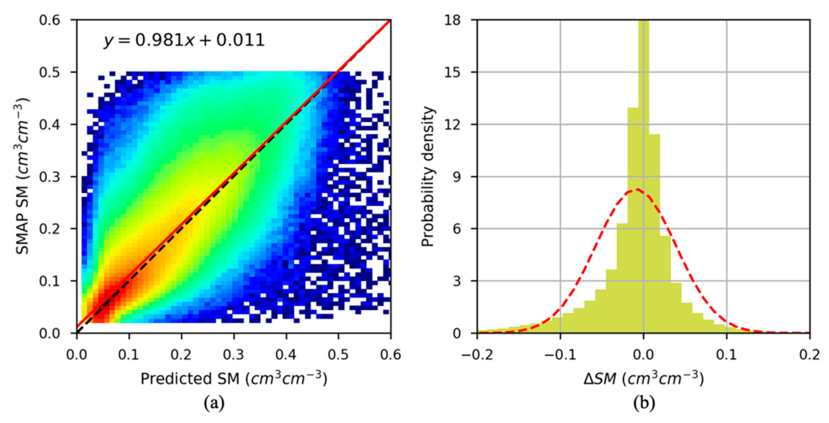
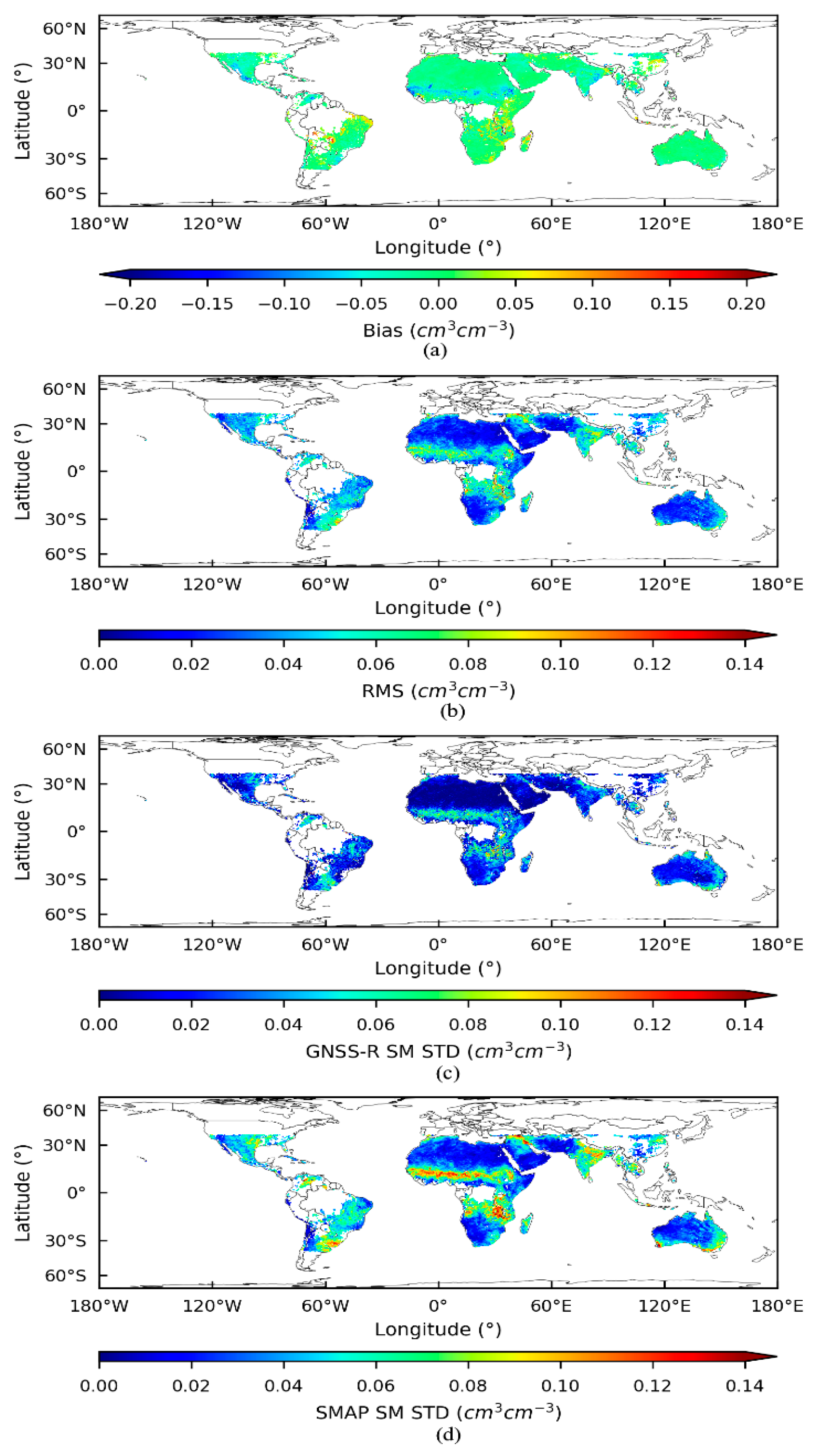
3.1. SSM Retrieval from GNSS-R

To evaluate the performance of the SSM retrieval algorithm, we conducted an experiment using the training dataset to regress the GNSS-R-derived effective reflectivity without vegetation and surface roughness correction. Regression was performed by generating a linear model for each EASE-Grid2 grid cell using the half-year spatial average effective reflectivity and SSM from the SMAP product. Figure 5 displays the resulting slope of the linear model was relatively smaller in arid regions where effective reflectivity was very low and soil moisture content was small and stable, whereas the intercept tended to be negative in such regions. Figure 5b clearly illustrates this trend.

Figure 6 depicts the density scatterplot of the matched SMAP SSM and CYGNSS-derived SSM from the testing dataset and the retrieval error distribution. The black dashed line represents a 1:1 diagonal and the red line shows the linear regression line in Figure 6a. The total number of SSM data pairs matched for model testing was 7,736,769. The results indicated that the total bias and RMSD of the CYGNSS-derived SSM were 0.009 cm³cm⁻³ and 0.048 cm³cm⁻³, respectively. The slope of the linear regression equation between the reference SSM and the inversed SSM was 0.981, and the scatter points were closely aligned with the linear regression line, suggesting a good match between the two datasets. The distribution of bias mainly falls between −0.05 cm³cm⁻³ and 0.05 cm³cm⁻³, confirming the accuracy of the retrieval model.

Figure 7a,b show the spatial map of the relative errors between the CYGNSS-retrieved SSM and SMAP SSM for each EASE-Grid2 grid cell from the testing dataset. The blue area indicates where GNSS-R underestimates the surface SSM, whereas the red area represents where it overestimates the SSM. In Figure 7a, the average bias is essentially small and mainly falls between −0.05 cm³cm⁻³ and 0.05 cm³cm⁻³. Figure 7b shows that the soil moisture inversion accuracy is less than 0.06 cm³cm⁻³ in most areas, except for a few wetter regions such as the Sudanian Savanna and Peninsular India. However, the standard deviations (STD) of CYGNSS-derived SSM and SMAP SSM in the last half-year of 2018 as shown in Figure 7c,d, respectively, indicate good consistency, demonstrating that CYGNSS can detect daily variation in soil moisture. Nonetheless, large deviations still exist in some areas, such as central and eastern parts of South America and central Africa.

3.2. Effects of Vegetation and Roughness

This section evaluates the performance of three retrieval configurations under different land cover types defined by the International Geosphere-Biosphere Programme (IGBP) to assess the impact of vegetation and surface roughness on the quality of CYGNSS-derived SSM. The first configuration involves directly using effective reflectivity to construct retrieval models, ignoring the effects of vegetation and roughness, as described in Section 3.1. The second configuration modifies the specular effective reflectivity with vegetation transmissivity for vegetation attenuation, using Equation (5). The third configuration further corrects for surface roughness attenuation using the roughness coefficient in Equation (6).

Compared to the first configuration, the accuracy of the retrieved SSM improved marginally when the effective reflectivity was modified with the vegetation effect. The bias and RMSD of the GNSS-R-derived SSM were 0.009 cm³cm⁻³ and 0.046 cm³cm⁻³, respectively. However, there was no significant improvement when the third configuration was utilized compared to the second configuration.

The retrieval accuracy of the GNSS-R SSM retrieval model over different land cover types was evaluated by comparing the results with those of the SMAP product. The statistical results are presented in

Table 1. CYGNSS soil moisture retrieval accuracy over different landcover types (unit: cm³cm⁻³).

Landcover ID	Land Classification	No Vegetation and Roughness Correction		Add Vegetation Correction		Add Vegetation and Roughness Correction
		Bias	RMSD	Bias	RMSD	Bias	RMSD
4	Deciduous-Broadleaf-Forest	−0.0040	0.0555	−0.0102	0.0544	−0.0100	0.0543
5	Mixed-Forest	−0.0083	0.0478	−0.0051	0.0466	−0.0051	0.0465
6	Closed Shrublands	−0.0058	0.0420	−0.0062	0.0408	−0.0060	0.0409
7	Open Shrublands	−0.0045	0.0345	−0.0048	0.0344	−0.0048	0.0344
8	Woody Savannas	−0.0090	0.0710	−0.0103	0.0679	−0.0102	0.0677
9	Savannas	−0.0028	0.0619	−0.0047	0.0579	−0.0047	0.0577
10	Grasslands	−0.0160	0.0580	−0.0164	0.0557	−0.0164	0.0556
11	Wetland	0.0025	0.0667	0.0012	0.0656	0.0014	0.0657
12	Croplands	−0.0188	0.0667	−0.0127	0.0606	−0.0126	0.0605
14	Cropland/Natural Vegetation Mosaics	−0.0314	0.0722	−0.0268	0.0707	−0.0264	0.0703
16	Barren	−0.0068	0.0285	−0.0068	0.0285	−0.0068	0.0285

. The highest retrieval error was found for the land cover with cropland/natural vegetation mosaics, and woody savannas, whereas barren and open shrublands showed the best inversion performance. The discrepancy in retrieval accuracy among different land cover types is partly due to the variation in the volume of local SSM content. After correcting for vegetation attenuation, the performance of the retrieval algorithm improved on vegetated terrain covered with deciduous-broadleaf-forest, mixed-forest, woody savannas, savannas, croplands, grasslands, and cropland/natural vegetation mosaics. The mean improvement was 4.4%. It is worth noting that the spatial resolution of the CYGNSS observations was higher than 36 km. Therefore, using the spatial average method for surface geophysical parameter processing instead of true values on the GNSS-R specular point may explain the lack of significant improvement with vegetation and roughness correction. Additionally, the uncertainty of the SMAP SSM product itself could have influenced the results.

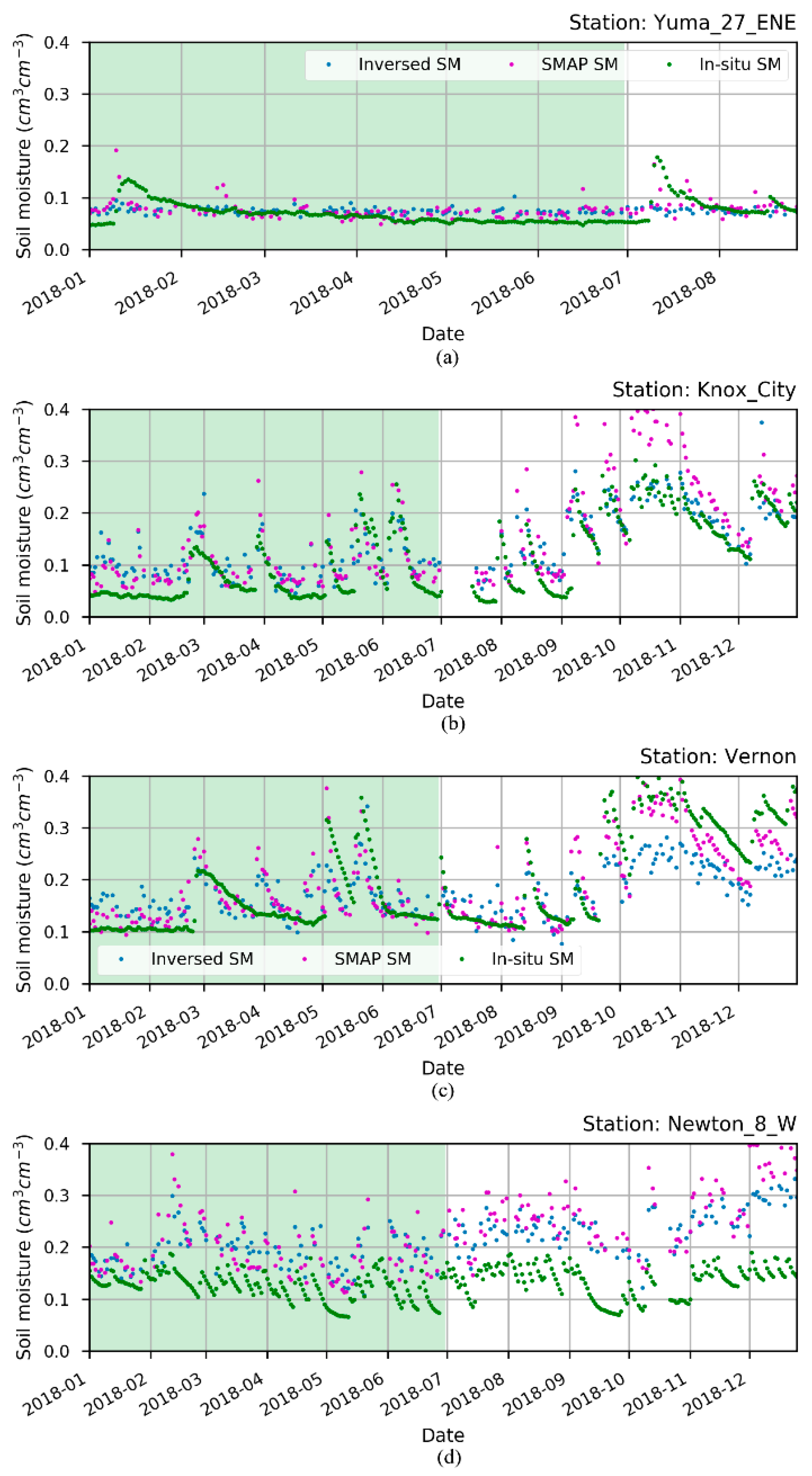
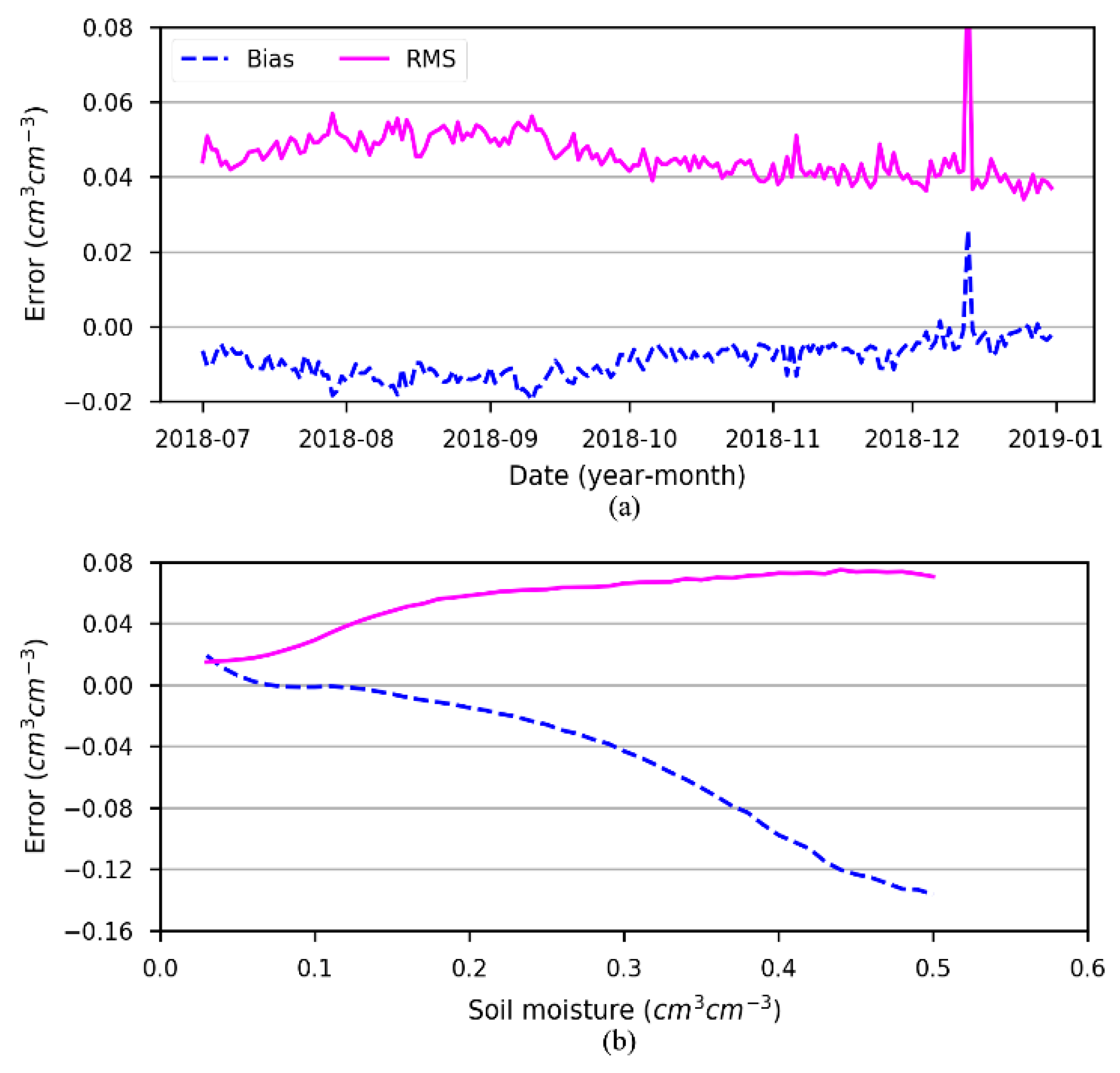
3.3. Validation of Soil Moisture by In Situ Observation

The reliability of the GNSS-R SSM retrieval methodology and the performance of attenuation correction were evaluated by comparing the results with in situ SSM data from the International Soil Moisture Network (ISMN). The in situ SSM measurements have a raw time resolution of 10 min and a probe depth of 0.0~0.05 m. To align the SSM data from different sources, the in situ measurements were resampled to a daily average value. The GNSS-R SSM values were selected for the nearest grid point values to the corresponding in situ station. Figure 8 compares the time series from the in situ SSM, SMAP SSM, and GNSS-R-derived SSM for both the training and testing data. The Yuma_27_ENE, Knox_City, and Vernon sites exhibited high consistency between the measured and predicted SSM. The predicted SSM from the developed linear model remained stable for six months of extrapolation, although there was a significant systematic difference between the predicted SSM and in situ measurements at the Newton_8_w station. This discrepancy may be due to representative errors for different spatial resolution scales.

Table 2. The CYGNSS soil moisture retrieval accuracy at different in situ stations (unit: cm³cm⁻³).

Station	Scene Name	No Vegetation and Roughness Correction		Add Vegetation Correction		Add Vegetation and Roughness Correction
		Bias	RMSD	Bias	RMSD	Bias	RMSD
Yuma_27_ENE	Open Shrubland	−0.015	0.030	−0.015	0.030	−0.015	0.030
Knox_City	Grassland	0.015	0.038	0.020	0.039	0.021	0.039
Vernon	Grassland	−0.051	0.069	−0.054	0.069	−0.053	0.070
Newton_8_W	Cropland	0.092	0.057	0.107	0.046	0.108	0.047

presents the validation results at the four different sites using various correction strategies. The Yuma_27_ENE station, located in a very arid area, exhibited relatively stable SSM levels throughout the year, and the CYGNSS-derived SSM also showed high stability. For the grassland stations of Knox_City and Vernon, the results showed a somewhat contradictory situation, with the retrieval model underestimating the last season of 2018 at Vernon. The model performed well at Knox_City, whereas the SMAP SSM exhibited the opposite behavior. The addition of attenuation corrections had an impact on the derived SSM at the two stations. At the Newton_8_w station, the vegetation correction improved the overall statistical RMSD value of the retrieved SSM, which was 0.082 cm³cm⁻³ compared to 0.076 cm³cm⁻³ for the SMAP SSM. Although there is a difference between global statistics due to the different spatial resolutions of the two datasets and the relatively small testing sample, the in situ validation confirms the ability of spaceborne GNSS-R reflectivity to sense changes in SSM compared to the SMAP radiometer. The systematic error for absolute SSM retrieval can be addressed using rescaling methods with larger datasets [36].

4. Discussion

This study reports on the results of the CYGNSS SSM retrieval algorithm and analyzes the performance of vegetation and surface roughness attenuation correction across different land cover types. The findings indicate that spaceborne GNSS-R can be used for SSM estimation, with the accuracy of CYGNSS-derived SSM being relatively stable. The daily CYGNSS-derived SSM shows small changes in temporal bias and RMSD against SMAP SSM during the testing period, as illustrated in Figure 9, with RMSD values of less than 0.06 cm³cm⁻³. This indicates the stability and reliability of the model. However, on 13 December 2018 there was a rapid increase in the bias and RMSD metrics, which was thought to be related to the CYGNSS observation quality on that day. The inversion error in various SSM bins shows that CYGNSS increasingly overestimates the ground SSM when the SSM is greater than 0.22 cm³cm⁻³. While the RMSD at different bins indicates a steady increase, the uncertainty remains stable at larger than 0.05 cm³cm⁻³ when the reference value is greater than 0.14 cm³cm⁻³. Based on the assessments conducted, it can be inferred that the accuracy of soil moisture estimates derived from CYGNSS is comparable to that of satellite-based radiometers.

In the retrieval of SSM using spaceborne GNSS-R, the dielectric properties of the land interface are affected by SSM, vegetation and surface roughness. The effective reflectivity of GNSS-R is directly related to its dielectric property. In regions with dense vegetation, vegetation attenuation can significantly impact SSM retrieval. While the tau-omega model has been used in previous research, it is not suitable for terrains with dense vegetation. To improve the accuracy of GNSS-R estimates, a better understanding of the scattering process over rough surfaces is necessary, and more reliable reference geophysical parameters must be selected. Furthermore, the entire GNSS-R inversion algorithm must be improved to accurately quantify the impact of other factors on retrieval accuracy. Vegetation correction improved the SSM inversion results from 0.048 cm³cm⁻³ to 0.046 cm³cm⁻³. However, when applying the correction method to various land cover types, the impact on CYGNSS SSM retrieval was not significant, indicating inconsistency with previous simulation results [37]. The limited improvement observed with the SMAP roughness parameter suggests that factors such as correction model, uncertainty in the SMAP parameters, and representation errors may have contributed to this outcome.

5. Conclusions

This study examines the potential of spaceborne GNSS-R for estimating land SSM. An empirical statistical model was developed using SMAP Level-3 SSM products as reference data. The accuracy of the CYGNSS-based retrievals of SSM was adversely affected by the attenuation effects of vegetation and surface roughness. However, after correcting for these effects, modest improvements were observed in SSM retrieval over vegetated areas. Nonetheless, the surface roughness correction method was found to be limited due to the absence of reliable small-scale surface roughness data and refined correction methods. The derived SSM had an accuracy of 0.046 cm³cm⁻³ with vegetation correction. The retrieval model developed in this study demonstrated stable performance, as assessed using in situ and SMAP data. It is evident that the current state of spaceborne GNSS-R SSM remote sensing requires the use of external auxiliary data for statistical modeling, and the impact of additional terrestrial geophysical factors must be carefully quantified. Future research should focus on developing models for vegetation and surface roughness correction in satellite-based GNSS-R to improve our understanding of the effects of vegetation cover and surface roughness on soil moisture variability over different land cover types. This study contributes to the advancement of remote sensing technology for soil moisture measurements.

References

1. Robock, A.; Vinnikov, K.Y.; Srinivasan, G.; Entin, J.K.; Hollinger, S.E.; Speranskaya, N.A.; Liu, S.; Namkhai, A. The Global Soil Moisture Data Bank. Bull. Am. Meteor. Soc. 2000, 81, 1281–1299. [Google Scholar] [CrossRef]
2. Kerr, Y.H.; Waldteufel, P.; Wigneron, J.-P.; Delwart, S.; Cabot, F.; Boutin, J.; Escorihuela, M.-J.; Font, J.; Reul, N.; Gruhier, C.; et al. The SMOS Mission: New Tool for Monitoring Key Elements of the Global Water Cycle. Proc. IEEE 2010, 98, 666–687. [Google Scholar] [CrossRef] [Green Version]
3. Brown, M.E.; Escobar, V.; Moran, S.; Entekhabi, D.; O’Neill, P.E.; Njoku, E.G.; Doorn, B.; Entin, J.K. NASA’s Soil Moisture Active Passive (SMAP) Mission and Opportunities for Applications Users. Bull. Am. Meteorol. Soc. 2013, 94, 1125–1128. [Google Scholar] [CrossRef]
4. Jin, S.; Su, K. PPP Models and Performances from Single- to Quad-Frequency BDS Observations. Satell. Navig. 2020, 1, 16. [Google Scholar] [CrossRef]
5. Martin-Neira, M.; Caparrini, M.; Font-Rossello, J.; Lannelongue, S.; Vallmitjana, C.S. The PARIS Concept: An Experimental Demonstration of Sea Surface Altimetry Using GPS Reflected Signals. IEEE Trans. Geosci. Remote Sens. 2001, 39, 142–150. [Google Scholar] [CrossRef] [Green Version]
6. Gleason, S.; Hodgart, S.; Sun, Y.; Gommenginger, C.; Mackin, S.; Adjrad, M.; Unwin, M. Detection and Processing of Bistatically Reflected GPS Signals from Low Earth Orbit for the Purpose of Ocean Remote Sensing. IEEE Trans. Geosci. Remote Sens. 2005, 43, 1229–1241. [Google Scholar] [CrossRef] [Green Version]
7. Jin, S.; Komjathy, A. GNSS Reflectometry and Remote Sensing: New Objectives and Results. Adv. Space Res. 2010, 46, 111–117. [Google Scholar] [CrossRef] [Green Version]
8. Njoku, E.G.; Entekhabi, D. Passive Microwave Remote Sensing of Soil Moisture. J. Hydrol. 1996, 184, 101–129. [Google Scholar] [CrossRef]
9. Egido, A.; Caparrini, M.; Ruffini, G.; Paloscia, S.; Santi, E.; Guerriero, L.; Pierdicca, N.; Floury, N. Global Navigation Satellite Systems Reflectometry as a Remote Sensing Tool for Agriculture. Remote Sens. 2012, 4, 2356–2372. [Google Scholar] [CrossRef] [Green Version]
10. Egido, A.; Paloscia, S.; Motte, E.; Guerriero, L.; Pierdicca, N.; Caparrini, M.; Santi, E.; Fontanelli, G.; Floury, N. Airborne GNSS-R Polarimetric Measurements for Soil Moisture and Above-Ground Biomass Estimation. IEEE J. Sel. Top. Appl. Earth Obs. Remote Sens. 2014, 7, 1522–1532. [Google Scholar] [CrossRef]
11. Ban, W.; Yu, K.; Zhang, X. GEO-Satellite-Based Reflectometry for Soil Moisture Estimation: Signal Modeling and Algorithm Development. IEEE Trans. Geosci. Remote Sens. 2018, 56, 1829–1838. [Google Scholar] [CrossRef]
12. Rodriguez-Alvarez, N.; Bosch-Lluis, X.; Camps, A.; Vall-llossera, M.; Valencia, E.; Marchan-Hernandez, J.F.; Ramos-Perez, I. Soil Moisture Retrieval Using GNSS-R Techniques: Experimental Results Over a Bare Soil Field. IEEE Trans. Geosci. Remote Sens. 2009, 47, 3616–3624. [Google Scholar] [CrossRef]
13. Foti, G.; Gommenginger, C.; Jales, P.; Unwin, M.; Shaw, A.; Robertson, C.; Roselló, J. Spaceborne GNSS Reflectometry for Ocean Winds: First Results from the UK TechDemoSat-1 Mission. Geophys. Res. Lett. 2015, 42, 5435–5441. [Google Scholar] [CrossRef] [Green Version]
14. Ruf, C.; Chang, P.; Clarizia, M.P.; Gleason, S.; Jelenak, Z.; Murray, J.; Morris, M.; Musko, S.; Posselt, D.; Provost, D.; et al. CYGNSS Handbook Cyclone Global Navigation Satellite System: Deriving Surface Wind Speeds in Tropical Cyclones; National Aeronautics and Space Administration: Ann Arbor, MI, USA, 2016; p. 154. ISBN 978-1-60785-380-0.
15. Chew, C.; Shah, R.; Zuffada, C.; Hajj, G.; Masters, D.; Mannucci, A.J. Demonstrating Soil Moisture Remote Sensing with Observations from the UK TechDemoSat-1 Satellite Mission. Geophys. Res. Lett. 2016, 43, 3317–3324. [Google Scholar] [CrossRef] [Green Version]
16. Camps, A.; Park, H.; Pablos, M.; Foti, G.; Gommenginger, C.P.; Liu, P.-W.; Judge, J. Sensitivity of GNSS-R Spaceborne Observations to Soil Moisture and Vegetation. IEEE J. Sel. Top. Appl. Earth Obs. Remote Sens. 2016, 9, 4730–4742. [Google Scholar] [CrossRef] [Green Version]
17. Camps, A.; Vall·llossera, M.; Park, H.; Portal, G.; Rossato, L. Sensitivity of TDS-1 GNSS-R Reflectivity to Soil Moisture: Global and Regional Differences and Impact of Different Spatial Scales. Remote Sens. 2018, 10, 1856. [Google Scholar] [CrossRef] [Green Version]
18. Ruf, C.S.; Chew, C.; Lang, T.; Morris, M.G.; Nave, K.; Ridley, A.; Balasubramaniam, R. A New Paradigm in Earth Environmental Monitoring with the CYGNSS Small Satellite Constellation. Sci. Rep. 2018, 8, 8782. [Google Scholar] [CrossRef] [Green Version]
19. Carreno-Luengo, H.; Luzi, G.; Crosetto, M. Sensitivity of CyGNSS Bistatic Reflectivity and SMAP Microwave Radiometry Brightness Temperature to Geophysical Parameters Over Land Surfaces. IEEE J. Sel. Top. Appl. Earth Obs. Remote Sens. 2019, 12, 107–122. [Google Scholar] [CrossRef]
20. Eroglu, O.; Kurum, M.; Ball, J.E. Preliminary Results of a GNSS-R Simulation to Sense Canopy Parameters. In Proceedings of the 2018 International Conference on Electromagnetics in Advanced Applications (ICEAA), Cartagena, Colombia, 10–14 September 2018; pp. 421–424. [Google Scholar]
21. Ferrazzoli, P.; Guerriero, L.; Pierdicca, N.; Rahmoune, R. Forest Biomass Monitoring with GNSS-R: Theoretical Simulations. Adv. Space Res. 2011, 47, 1823–1832. [Google Scholar] [CrossRef]
22. Kurum, M.; Deshpande, M.; Joseph, A.T.; O’Neill, P.E.; Lang, R.H.; Eroglu, O. SCoBi-Veg: A Generalized Bistatic Scattering Model of Reflectometry from Vegetation for Signals of Opportunity Applications. IEEE Trans. Geosci. Remote Sens. 2019, 57, 1049–1068. [Google Scholar] [CrossRef]
23. Chew, C.C.; Small, E.E. Soil Moisture Sensing Using Spaceborne GNSS Reflections: Comparison of CYGNSS Reflectivity to SMAP Soil Moisture. Geophys. Res. Lett. 2018, 45, 4049–4057. [Google Scholar] [CrossRef] [Green Version]
24. Clarizia, M.P.; Pierdicca, N.; Costantini, F.; Floury, N. Analysis of CYGNSS Data for Soil Moisture Retrieval. IEEE J. Sel. Top. Appl. Earth Obs. Remote Sens. 2019, 12, 2227–2235. [Google Scholar] [CrossRef]
25. Eroglu, O.; Kurum, M.; Boyd, D.; Gurbuz, A.C. High Spatio-Temporal Resolution CYGNSS Soil Moisture Estimates Using Artificial Neural Networks. Remote Sens. 2019, 11, 2272. [Google Scholar] [CrossRef] [Green Version]
26. Dobson, M.; Ulaby, F.; Hallikainen, M.; El-rayes, M. Microwave Dielectric Behavior of Wet Soil-Part II: Dielectric Mixing Models. IEEE Trans. Geosci. Remote Sens. 1985, GE-23, 35–46. [Google Scholar] [CrossRef]
27. Zavorotny, V.U.; Voronovich, A.G. Scattering of GPS Signals from the Ocean with Wind Remote Sensing Application. IEEE Trans. Geosci. Remote Sens. 2000, 38, 951–964. [Google Scholar] [CrossRef] [Green Version]
28. Al-Khaldi, M.M.; Johnson, J.T.; O’Brien, A.J.; Balenzano, A.; Mattia, F. Time-Series Retrieval of Soil Moisture Using CYGNSS. IEEE Trans. Geosci. Remote Sens. 2019, 57, 4322–4331. [Google Scholar] [CrossRef]
29. Camps, A. Spatial Resolution in GNSS-R Under Coherent Scattering. IEEE Geosci. Remote Sens. Lett. 2020, 17, 32–36. [Google Scholar] [CrossRef] [Green Version]
30. Chew, C.; Reager, J.T.; Small, E. CYGNSS Data Map Flood Inundation during the 2017 Atlantic Hurricane Season. Sci. Rep. 2018, 8, 9336. [Google Scholar] [CrossRef]
31. Gleason, S.; Ruf, C.S.; Clarizia, M.P.; O’Brien, A.J. Calibration and Unwrapping of the Normalized Scattering Cross Section for the Cyclone Global Navigation Satellite System. IEEE Trans. Geosci. Remote Sens. 2016, 54, 2495–2509. [Google Scholar] [CrossRef]
32. Azemati, A.; Moghaddam, M. Moghaddam Modeling and Analysis of Bistatic Scattering from Forests in Support of Soil Moisture Retrieval. In Proceedings of the 2017 IEEE International Symposium on Antennas and Propagation & USNC/URSI National Radio Science Meeting, San Diego, CA, USA, 9 July 2017; pp. 1833–1834. [Google Scholar]
33. Jackson, T.J.; Schmugge, T.J. Vegetation Effects on the Microwave Emission of Soils. Remote Sens. Environ. 1991, 36, 203–212. [Google Scholar] [CrossRef]
34. Campbell, J.D.; Moghaddam, M. GNSS-R Parameter Sensitivities for Soil Moisture Retrieval. In Proceedings of the 2018 International Conference on Electromagnetics in Advanced Applications (ICEAA), Cartagena, Colombia, 10–14 September 2018; pp. 609–612. [Google Scholar]
35. Kerr, Y.H.; Waldteufel, P.; Wigneron, J.-P.; Martinuzzi, J.; Font, J.; Berger, M. Soil Moisture Retrieval from Space: The Soil Moisture and Ocean Salinity (SMOS) Mission. IEEE Trans. Geosci. Remote Sens. 2001, 39, 1729–1735. [Google Scholar] [CrossRef]
36. Gruber, A.; De Lannoy, G.; Albergel, C.; Al-Yaari, A.; Brocca, L.; Calvet, J.-C.; Colliander, A.; Cosh, M.; Crow, W.; Dorigo, W.; et al. Validation Practices for Satellite Soil Moisture Retrievals: What Are (the) Errors? Remote Sens. Environ. 2020, 244, 111806. [Google Scholar] [CrossRef]
37. Pierdicca, N.; Guerriero, L.; Brogioni, M.; Egido, A. On the Coherent and Non Coherent Components of Bare and Vegetated Terrain Bistatic Scattering: Modelling the GNSS-R Signal over Land. In Proceedings of the 2012 IEEE International Geoscience and Remote Sensing Symposium, Munich, Germany, 22–27 July 2012; pp. 3407–3410. [Google Scholar]
Figure 1. Averaged SMAP Level-3 soil moisture from satellite descending passes and ascending passes on 1 January 2018.
Atmosphere 14 00509 g001
Figure 2. Complex permittivity under different soil moisture (a) and the relationship between soil moisture and reflectivity at the different signal incidence angle (b).
Atmosphere 14 00509 g002
Figure 3. Bistatic radar geometry of spaceborne GNSS-R remote sensing soil detection.
Atmosphere 14 00509 g003
Figure 4. Spaceborne GNSS-R SSM retrieval algorithm flow chart.
Atmosphere 14 00509 g004
Figure 5. The slope (a) and intercept (b) of the linear SSM retrieval model.
Atmosphere 14 00509 g005
Figure 6. Density scatterplot of GNSS-R derived SSM and SMAP SSM (a) and probability density distribution of inversed SSM deviation (b).
Atmosphere 14 00509 g006
Figure 7. Bias (a) and RMS (b) of GNSS-R retrieved SSM, STD of SMAP SSM (c) and GNSS-R inversed SSM (d).
Atmosphere 14 00509 g007
Figure 8. Time series of inversed SSM, SMAP SSM, and in situ SSM comparison at in situ SSM stations Yuma-27-ENE (a), Knox City (b), Vernon (c), and Newton-8-W (d).
Atmosphere 14 00509 g008
Figure 9. Testing data daily error statistic (a) and total retrieval error at different soil moisture bins (b).
Atmosphere 14 00509 g009