Methodology for Mobile Toxics Deterministic Human Health Risk Assessment and Case Study

Abstract

Air toxic emissions from on-road mobile sources are significant contributors to the degradation of air quality in urban and dense population centers. Research led by the United States Environmental Protection Agency (EPA) identified more than 1162 hazardous air pollutants (HAPs) in the exhaust and evaporative emissions from on-road mobile sources. However, less than 70 hazardous air pollutants are monitored by regulatory agencies. HAPs emitted from Mobile Sources are known as Mobile Source Air Toxics (MSATs). The EPA estimates that approximately half of the cancer risk and 74% of noncancer health impacts from air toxics is attributed to mobile sources. The quantification of the risk associated with MSATs exposure remains limited to date, and only a few MSATs have ambient air quality standards to protect human health and welfare. This work presents a novel and validated methodology to quantify the myriad health risks associated with exposure to on-road mobile emissions. This methodology is introduced in the form of a pipelined analysis process, which may be employed in existing and new transportation projects. The proposed new methodology integrates results from three different types of models: on-road vehicle emissions inventory models such as MOVES and IVE, air dispersion models such as AERMOD and SCIPUFF, and risk estimate models for human and ecological receptors such as the 2005 Final U.S. EPA Human Health Risk Assessment Protocol for Hazardous Waste Combustion Facilities. The result of this research work is a new methodology that provides regulators and risk analysts with a more detailed awareness of the health impacts of MSATs. A case study of Saint Paul, Minnesota, validated the air dispersion modeled results against monitored data, and the agreement was acceptable (i.e., the estimates were within a factor of two of the observations). Three high-population locations in the Saint Paul area were evaluated for human health risk, with the observation that at two of these locations, the Saint Paul—Ramsey Health Center and Anderson Office Building, the calculated cancer risk is in excess of the target risk level of 1.0E-05 for benzo(a)pyrene. The methodology presented in this paper allows regulators, risk analysts, and air quality engineers to better estimate multi-pathway cancer and noncancer risk associated with acute and chronic exposure to MSATs. Moreover, this work provides a science-based aid to policy decision makers when considering factors that most significantly affect population health and ecology.

1. Introduction

In 2012, the World Health Organization (WHO) estimated that 7 million premature deaths per year were caused by exposure to air pollution [1]. Exposure to air pollution causes adverse effects such as strokes, chronic obstructive pulmonary disease (COPD), acute lower respiratory infections, and lung cancer [2]. In addition to the alarming numbers published in the WHO report, more than 43% of Americans live in areas with poor air quality, putting their lives at risk [3]. Air pollution costs the global economy trillions of dollars annually due to healthcare expenditures and lost work and is one of the leading causes of morbidity and mortality [4,5].

Sources of air pollution are of biogenic and anthropogenic origins, such as emissions resulting from energy production by combustion, industrial processes, metallurgical industry, residential heating, waste treatment, and mobile sources. Mobile sources are divided into two categories: on-road, including trucks, passenger cars, buses, and motorcycles, and non-road, including commercial marine vessels, airplanes, railroads, agricultural tools, snow equipment, and recreational vehicles. On-road mobile sources emit more than 1162 compounds into the atmosphere via tailpipe and evaporative emissions [6,7].

On-road mobile sources, which are the focus of this paper, also emit non-exhaust emissions from the release of gasoline vapor in the fuel storage system [8], fluid leaks (e.g., fuel, lubricants, and refrigerants), particulate matter from brake dust and tire wear, and re-entrained road dust [9].

Numerous peer-reviewed studies have clearly demonstrated that mobile source emissions are the most significant contributor to air pollution in urban areas, and they represent a risk to human and ecological health [10,11,12,13,14,15].

In addition to the previously mentioned studies, the 2014 National Air Toxics Assessment (NATA), the EPA’s most recent large-scale and recurring risk assessment, showed that the United States national cancer risk from exposure to air toxics emitted from on-road sources was approximately “4-in-1 million” [16]. This means that if one million people were exposed to the same concentration of MSATs continuously over 70 years, four people would likely contract cancer from this exposure. On-road sources contributed to 12.43% of the 2014 NATA national cancer risk by source groups (NCRSG) as the second leading contributor.

In the United States, more than 13% of the population live, attend school, or work within 100 m of a major road [17]. Kingsley et al. [18] showed that in 2005–2006, more than 6 million students attended schools within 250 m of a major road.

MSATs and criteria pollutant concentrations are higher near the roadway, with the maximum concentrations typically occurring within the first 100 to 150 m of a roadway [19,20]. For example, according to the Mobile Source Air Toxics report published by the Health Effects Institute [6], near-road monitoring and air monitoring network data showed that the highest levels of ambient benzene and formaldehyde concentrations were measured at urban roadside monitors.

Depending on many factors, such as the air toxics chemical structure, daily meteorological conditions, vehicle fleet mix, presence of barriers, and the terrain surrounding the roadway, ambient concentrations of MSATs can be found within 600 m of a roadway [19]. Additionally, the EPA’s transportation conformity and hot-spot guidance recommend placing air dispersion modeling calculation points (receptors) to estimate concentration impacts at distances as close as five meters from a roadway edge [21].

Unlike criteria pollutants, air toxics lack effective ambient air quality standards or guidelines in Canada or the United States that are directly applicable to protecting public health or the surrounding environment [22,23]. Moreover, regulatory agencies around the world do not monitor the vast majority of air toxics but monitor only a small fraction, less than 70, of the list of thousands of air toxics being emitted from on-road sources [24,25].

This work employs the chronic and acute toxicity approach [26] to estimate the multi-pathway cancer risk and noncancer hazard from exposure to MSATs. This approach, coupled with air dispersion modeling and estimation of population exposures, addresses the absence of ambient air quality standards for most of the MSATs and the lack of monitoring by regulatory agencies by determining through modeling the health impacts resulting from extended and acute exposure to MSATs.

Humans (also known as human receptors) may come into contact with air toxics via two main exposure routes or pathways: (1) direct via inhalation and (2) indirect via ingestion of contaminated water, produce, and animals. Examples of indirect pathways include deposition of air toxics onto the soil and produce such as lettuce and tomatoes. Additionally, biotic uptake and accumulation from contaminated soil or water can occur, such as irrigation water transporting soil deposits containing air toxics and resulting in uptake by fish and livestock, including cattle, swine, chickens, and sheep. In addition, the incidental ingestion of soil itself is considered an important indirect exposure pathway. Soil contamination is attributed to direct discharge to the soil, atmospheric deposition of air toxics, or transport from other media (e.g., through runoff). Consideration of indirect exposure pathways is critical for certain air toxics. For example, the indirect risk from dioxin and furans can be orders of magnitude higher than the direct risk [27]. Heavy-duty diesel vehicles emit furans and dioxins [28,29,30,31]. Furans and dioxins are highly toxic compounds that contain the dibenzofuran nucleus and dibenzo-p-dioxin nucleus, respectively. 2,3,7,8-Tetrachlorodibenzodioxin (TCDD) is the most toxic and most comprehensively studied dioxin [32]. Moreover, TCDD is highly lipophilic and tends to bioaccumulate in the food chain [33], thereby presenting a potentially elevated risk through the consumption of food exposed to TCDD, further contributing to the risk already caused by inhalation exposure to MSATs.

This work presents a novel and practical (streamlined and integrated) methodology to assess the significant human health impacts associated with chronic and acute exposure to MSATs by calculating the total inhalation cancer risk and the total inhalation hazard quotient. Furthermore, this methodology computes the cumulative cancer risk and the air toxics hazard index due to exposure via indirect pathways such as ingestion. Finally, the methodology is verified using monitored data.

Literature Review

Previous work performed on assessing human health impacts from exposure to air toxics includes the National Air Toxics Assessment [16], Regional Air Impact Modeling Initiative [34,35], and MPCA Statewide Cumulative Risk Study [36], which are briefly described here.

The most recent large-scale and recurring risk assessment is the National Air Toxics Assessment (NATA). A NATA is conducted every three years, and the most current one is from 2017. NATAs provide a snapshot of the outdoor air quality and risks associated with exposure to air toxics. The main objective of the NATA is to identify air toxics that are of the highest potential concern in terms of contribution to population risk. NATAs only focus on risks resulting from direct inhalation of air toxics rather than evaluating other indirect pathways, such as ingestion. Cancer and noncancer health effects are estimated from breathing air toxics at a constant concentration over a lifetime (i.e., 70 years). Results from the NATA are used in prioritizing pollutants and emission sources. The 2014 NATA results reported that cancer risk due to inhalation of MSATs was 12.43% of the national cancer risk by source groups [16], and this is equal to “4 in 1 million people”. This percentage does not include the cumulative cancer risk due to indirect exposure of MSATs, nor other noncancer health impacts such as damage to the central nervous system or cardiovascular disease. A NATA is not appropriate for identifying local-scale air toxics “hot spots”, nor is it appropriate for identifying localized risks or individual risks from air toxics from near-roadway-related exposures. Furthermore, NATAs do not include risks due to non-inhalation exposure pathways.

The Regional Air Impact Modeling Initiative (RAIMI) included development of a suite of integrated software tools and reports, developed under contract by Lakes Environmental Software for the EPA Region 6 Compliance Assurance and Enforcement Division [34]. The RAIMI program and tools were developed to conduct community-wide cumulative air dispersion and human health risk assessment modeling for hundreds of air toxics from thousands of air pollution sources. Human health risk assessment modeling involves evaluating chronic cancer risks, noncancer hazards, and short-term acute exposure and is conducted following the methodologies published in the Human Health Risk Assessment Protocol (HHRAP) for Hazardous Waste Combustion Facilities [26]. Exposure pathways include direct inhalation and multiple indirect pathways, such as water, plant, and animal tissue ingestion. The first RAIMI pilot study was conducted in Harris County, Texas [35], including the Houston Ship Channel industrial corridor. The most significant obstacle to the implementation of the RAIMI program was source parameterization (i.e., characterizing physical source parameters required to support air dispersion modeling). After preliminary modeling was completed, it was determined that many sources driving adverse human health risk were in fact fugitive sources, which required the development of necessary physical source parameters to model as fugitive sources instead of point sources as originally reported in the Texas Commission on Environmental Quality (TCEQ) emissions inventory database. The RAIMI was the first regional study to integrate all the necessary tools and peer-reviewed guidance required to conduct large-scale cumulative human health risk assessments. The project outcome resulted in the identification of multiple risk hotspots, where the EPA was able to utilize its regulatory authority to enforce existing permit limits and, where necessary, modify permits to ensure that emissions control or process changes were made to protect cumulative health impacts to the communities affected.

The dispersion of emissions from on-road sources cannot be accurately estimated using a single point source. This paper employs non-point sources to estimate the dispersion of pollution from a road network. Another weakness of the RAIMI program is the emissions inventory inputs. The RAIMI emissions inventories tend to follow the EPA’s AP-42 emission factors, and these emission factors are not up to date with the current science, such as improved fuel formulation with less sulfur content or efficient internal combustion engines equipped with advanced emission control technologies. The on-road mobile emissions inventory in the proposed methodology is prepared using the EPA’s state-of-the-science maintained Vehicle Emission Simulator called MOVES.

The Indiana Department of Environmental Management’s RAIMI study [12] demonstrated that the incremental cancer risk from exposure to MSATs was “18.6 in 1 million people”, and the cancer risk drivers were formaldehyde and benzene. Moreover, the highest noncancer risk was also due to MSAT exposure, with the noncancer risk driver being acrolein. Acrolein is a common air toxic, found in urban settings, that is emitted from motor vehicles [37].

The Minnesota Pollution Control Agency (MPCA) conducted a statewide screening level human health risk assessment study of all inventoried emission sources, including on-road mobile sources, non-road mobile sources, area (non-point sources), and permitted point sources located in Minnesota [36]. The MPCA conducted a cumulative risk study according to the methodologies and science in the HHRAP [26]. The statewide screening level human health risk assessment was conducted using the Minnesota statewide risk screening (MNRISKs) tool [36]. MNRISKs automates the process of compiling the emissions inventory by incorporating data for point, area, and mobile sources, air dispersion modeling, and risk assessment.

MNRISKS incorporates the AERMOD air dispersion model (American Meteorological Society (AMS)/United States Environmental Protection Agency (EPA) Regulatory Model) and risk assessment protocols outlined in the HHRAP to predict cancer risk and noncancer hazard indices.

The cumulative human risk study is updated for the entire state every three years, with a comprehensive emissions inventory of all source categories, including more than 12,271 industrial point source emissions processes, on-road and non-road mobile sources, and 18 subcategories of area sources. More than 250 pollutants from all source categories are included in the study.

Following the study by MPCA, a collection of peer-reviewed articles was published [11,13,38], confirming the necessity of evaluating emissions from on-road sources and how they contribute to adverse health effects resulting from acute and chronic exposure.

Numerous articles include the results from the two most recently published MNRISKS studies based on emissions for 2008 [11] and 2011 [13]. Using these studies, Pratt et al. [11] showed that on-road mobile sources contributed to the highest cancer risks within the 2008 MNRISKS study, with a cancer risk of 3.70E-04, which is equal to an increase in cancer incidence of “370 in 1 million people”. Additionally, exposure to MSATs contributed to the highest noncancer risk.

Pratt et al. [13] compared different source groups and concluded that nontraditional sources, such as on-road mobile sources, were important sources of human health risk. Furthermore, on-road mobile source contribution to cancer and noncancer endpoints was higher than point sources. The analysis of Pratt et al. [13] showed that formaldehyde, acrolein, and diesel particulate matter (DPM) were the inhalation cancer risk drivers, and these air toxics are found in motor vehicle exhaust. The maximum DPM inhalation cancer risk modeled using MNRISKS-AERMOD was equal to an increase in cancer incidence of “900 in 1 million people”.

One area for improving the MNRISKS study is the better characterization of emissions and health impacts from mobile sources by introducing spatiotemporal considerations, i.e., changes in space over time. An existing limitation in current air toxics risk analyses is the practice of only employing annual averages to classify motor vehicle emissions in space but with time averaged out. Annual averages miss important pathways for mobile toxic emissions. By adding hourly spatiotemporal capabilities to existing mobile source simulations, a better ability to predict specific area and time health impacts is achievable. Lastly, it is observed that all reviewed literature employs deterministic risk models. These deterministic models include average exposure assumptions, such as an adult body weight value of 70 kg, meaning the results do not capture the range of variability in cancer or noncancer health risk.

The literature reviewed in this section is summarized in

Table 1. Literature Review Summary.

Risk Program	Literature Review Summary
NATA	A U.S. nationwide human health risk assessment conducted every three years and only evaluating direct inhalation risk. NATA is not appropriate for identifying local-scale air toxics “hot-spot” risks resulting from near-roadway-related exposures. The 2014 NATA reports that on-road mobile sources contributed to 12.43% of the national cancer risk by source groups.
RAIMI	A multi-pathway assessment of human health risk program that involves evaluating chronic cancer risks, noncancer hazards, and short-term acute exposure and is conducted following the methodologies published in the Human Health Risk Assessment Protocol. The first RAIMI pilot study was conducted in Harris County, Texas, including the Houston Ship Channel industrial corridor.
MNRISKS	A Minnesota statewide cumulative risk program conducted every three years, with a comprehensive emissions inventory of all source categories, including more than 12,271 industrial point source emissions processes, on-road and non-road mobile sources, and 18 subcategories of area sources. The program evaluates direct inhalation risk and risks resulting from indirect exposure pathways such as produce and fish consumption.

.

2. Materials and Methods

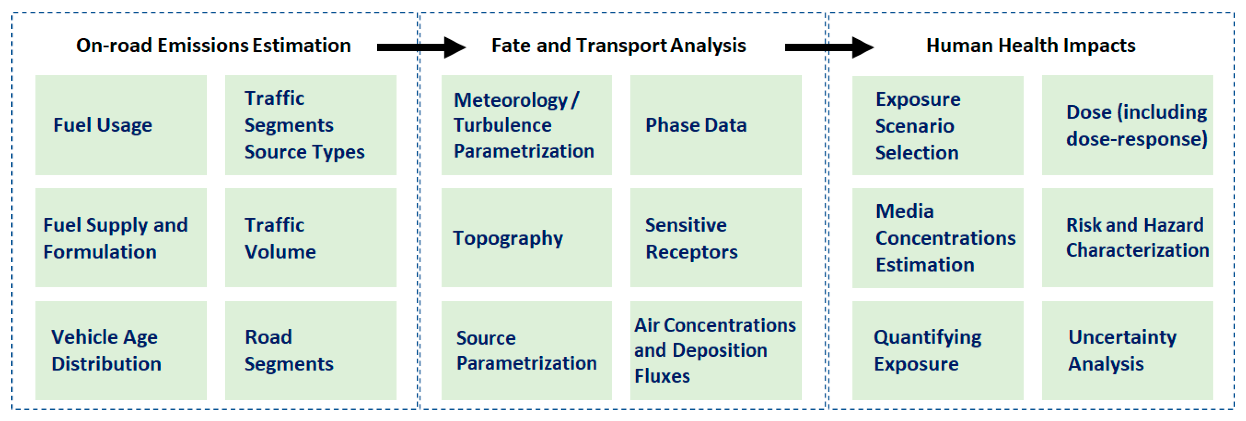
This work presents a novel and verified methodology to quantify the myriad health risks associated with exposure to on-road mobile emissions. Methodology verification is based on validated air dispersion results and observed trends being as expected. The methodology is summarized as follows:

• Estimate emissions from on-road vehicles using current U.S. regulatory models such as MOVES or similar vehicle emissions simulators.
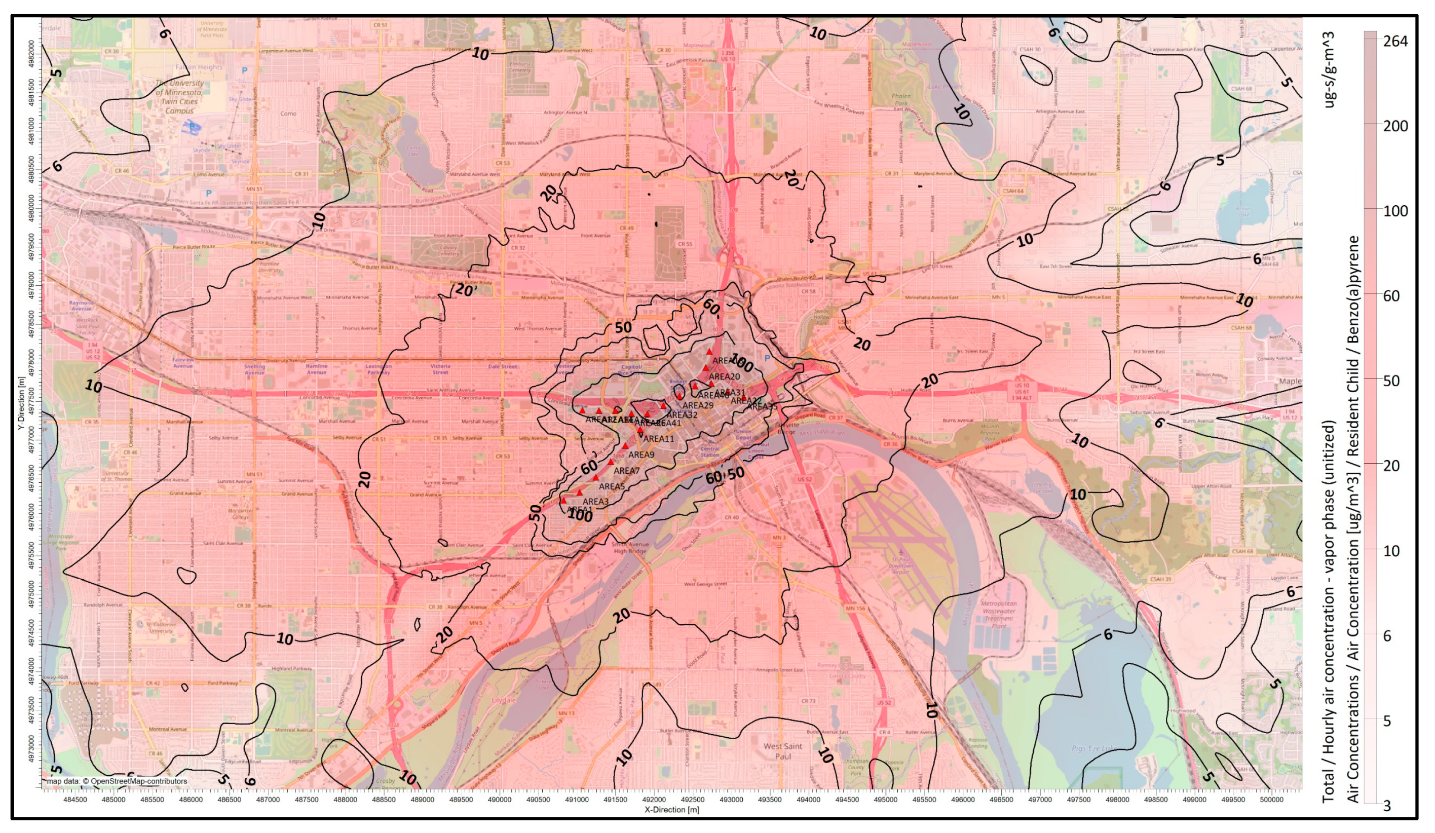
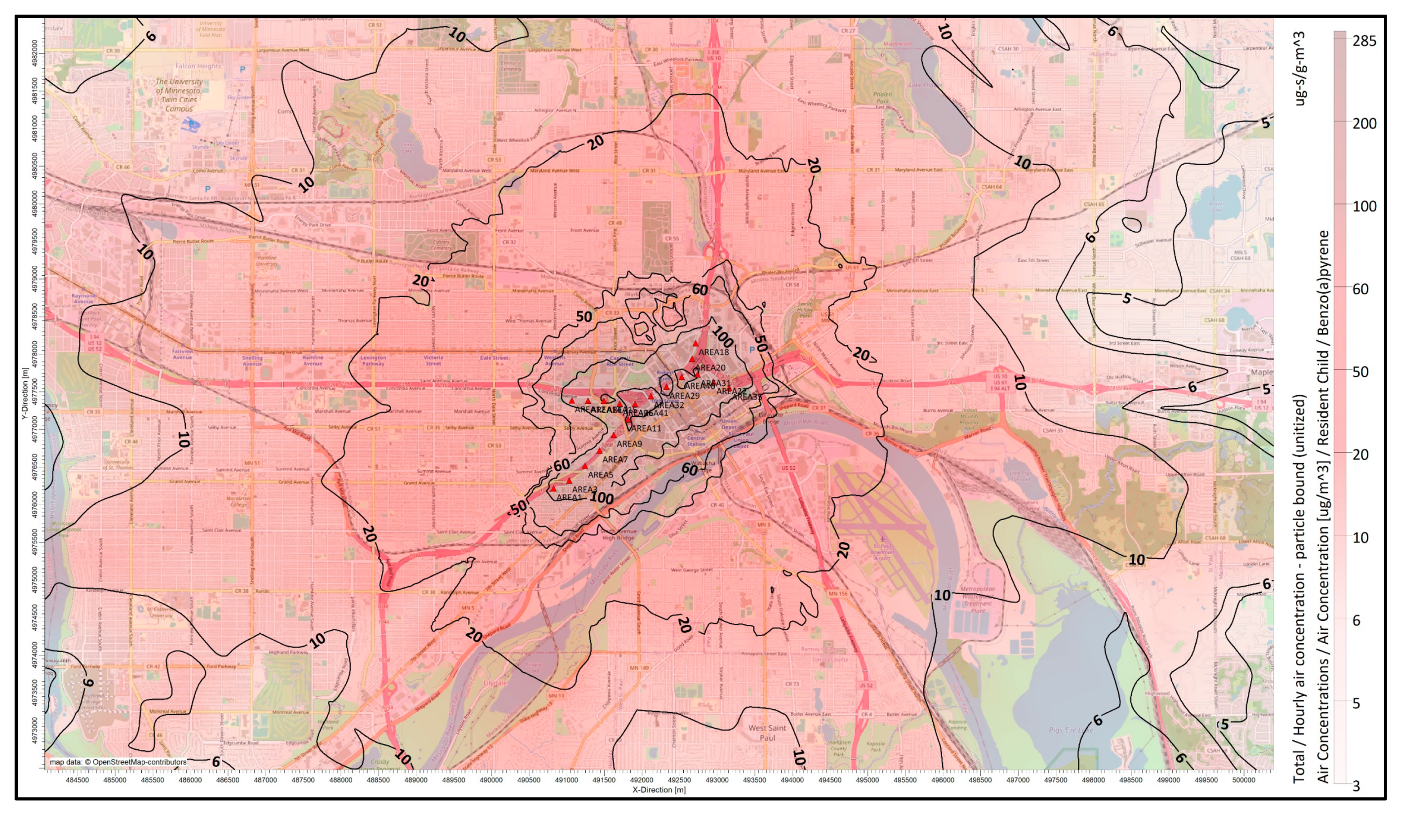
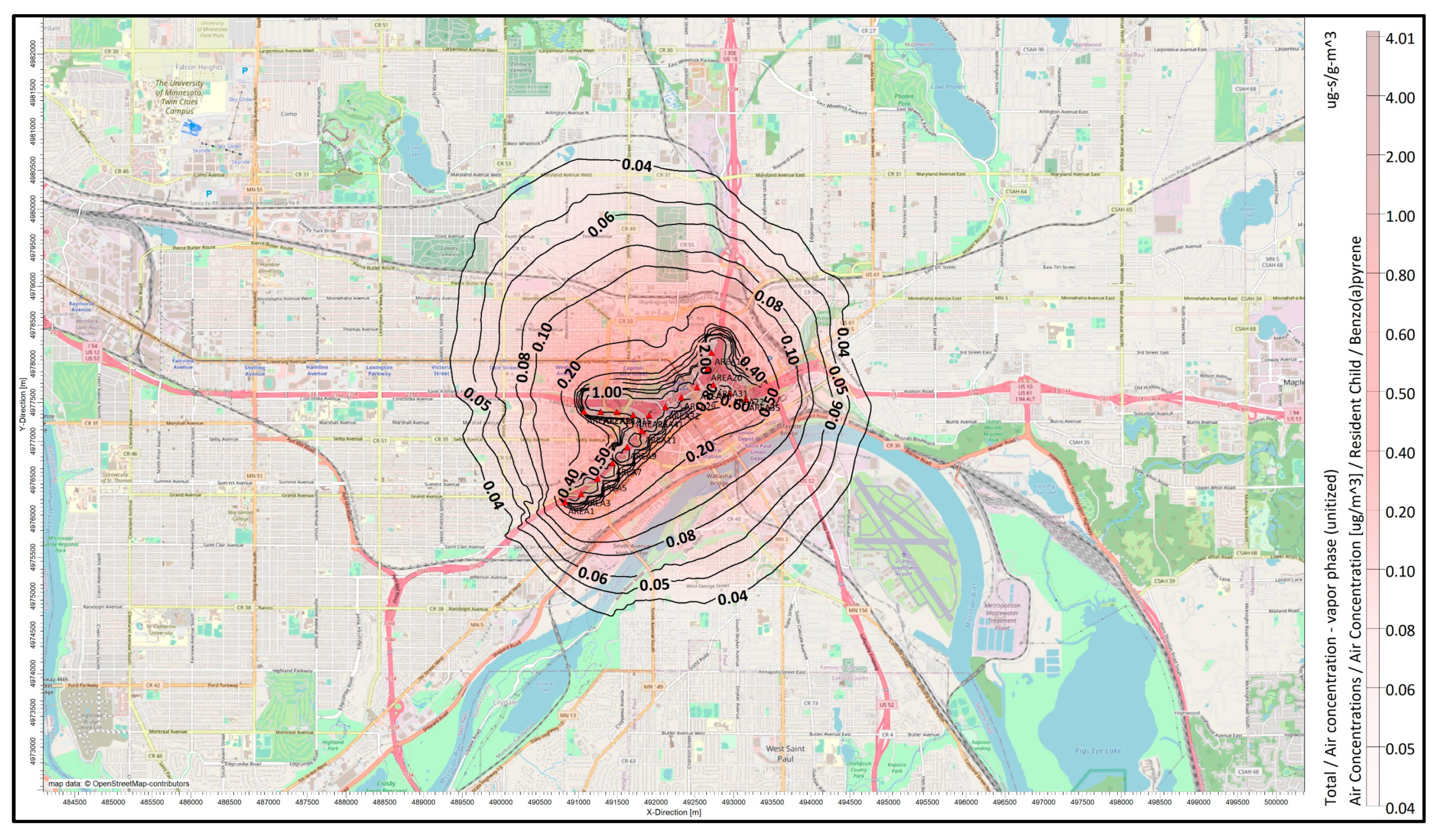
• Conduct air dispersion modeling using current U.S. regulatory air dispersion models, such as AERMOD or similar, to predict Mobile Source Air Toxics (MSATs) air concentrations and deposition to media, including soil and water.
• Determine critical air concentrations for each MSAT of interest.
• Identify through a multi-pathway fate-and-transport analysis the concentration of the MSATs in various exposure media, to evaluate indirect exposure pathways (e.g., deposition from air to soil, water, sediment, plants, and animal tissue) at sensitive locations of potential high impact.
• At each sensitive location, determine the total dose to humans from all pathways, i.e., direct inhalation and scenario-relevant indirect pathways.
• Conduct cumulative human health risk assessment to determine the total cancer and noncancer health effects for all-pathways based on the air toxics doses at each sensitive location (including acute and chronic exposure and direct and indirect exposure pathways).

Figure 1 shows the flowchart of the methodology.

Three MSATs, namely benzene, formaldehyde, and benzo(a)pyrene, were selected for this study. Though this a very small fraction of the MSATs, these three chemicals were selected due to their potency and the abundance of cancer and noncancer assessments in the literature.

Under the guidelines for carcinogen risk assessment, benzene is classified as a known human carcinogen [39]. Moreover, the international agency for research on cancer (IARC) has determined that exposure to benzene causes acute myeloid leukemia [40,41].

Formaldehyde is classified as a human carcinogen as per the findings published by IARC [42], and more recently, the United States Department of Health and Human Services (HHS) has categorized formaldehyde as a known human carcinogen [43]. IARC and EPA both classify benzo(a)pyrene (BaP) as carcinogenic to humans [44,45].

Due to the proximity of human activity near busy and congested roads, humans are exposed to high ambient concentrations of MSATs such as benzene and other potent Polycyclic Aromatic Hydrocarbons (PAHs) [46] for extended periods.

Furthermore, traffic emissions are particularly rich in ultrafine and nanoparticles that can easily enter the bloodstream and affect multiple organ systems. They can even directly penetrate the brain via the olfactory bulb [47].

2.1. On-Road Vehicle Emissions Inventory

In this work, the vehicle emissions inventory is prepared using the EPA’s state-of-the-science Motor Vehicle Emission Simulator called MOVES [48]. The version used in this work is MOVES2014b, embedded in the TRAQS system [49].

MOVES2014b estimates the emission factors and emission inventories for the following pollutants: particulate matter (PM10 and PM2.5), nitrous oxides (NOx), sulfur dioxide (SO2), carbon monoxide (CO), greenhouse gases (GHGs), metals, and MSATs, which are the focus of this work. MOVES2014b is capable of modeling continuous releases of MSATs with over 50 different exhaust and evaporative species. Moreover, the simulator accounts for various fuel types (e.g., diesel, gasoline, E85) used by various mobile sources, such as cars, buses, motorcycles, and haul trucks. Furthermore, the simulator includes different emission rates for each combination of sources, age groups, and operating modes, and it accurately reflects the various vehicle operating processes, such as running exhaust, crankcase running exhaust, cold start, or extended idle, and provides estimates of bulk emissions or emission rates. It is important to note that the availability and completeness of an on-road emissions inventory are crucial to assess the deleterious effects of MSATs.

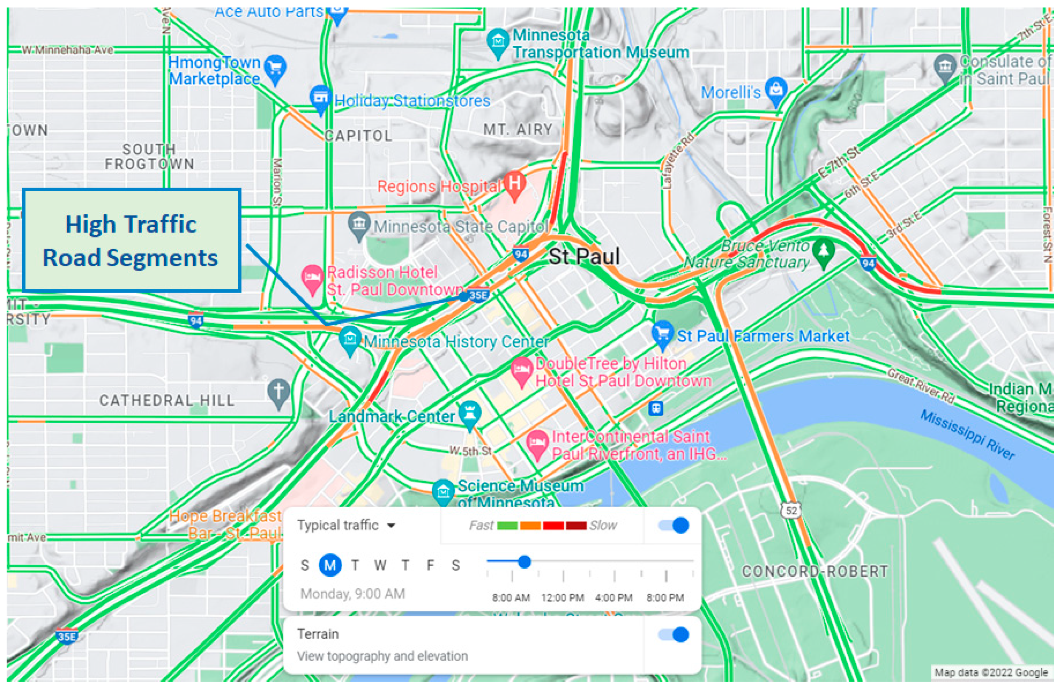
Vehicle emissions for this work were generated at the road-segment level. MOVES2014b requires data on road segments as well as vehicle classes, including motorcycles, light-duty vehicles, buses, single-unit trucks, and combination trucks. Additionally, the simulator requires information such as fuel specifications and usage, vehicle age distribution, traffic volume, and meteorology.

2.2. Roadway Geometry Characterization

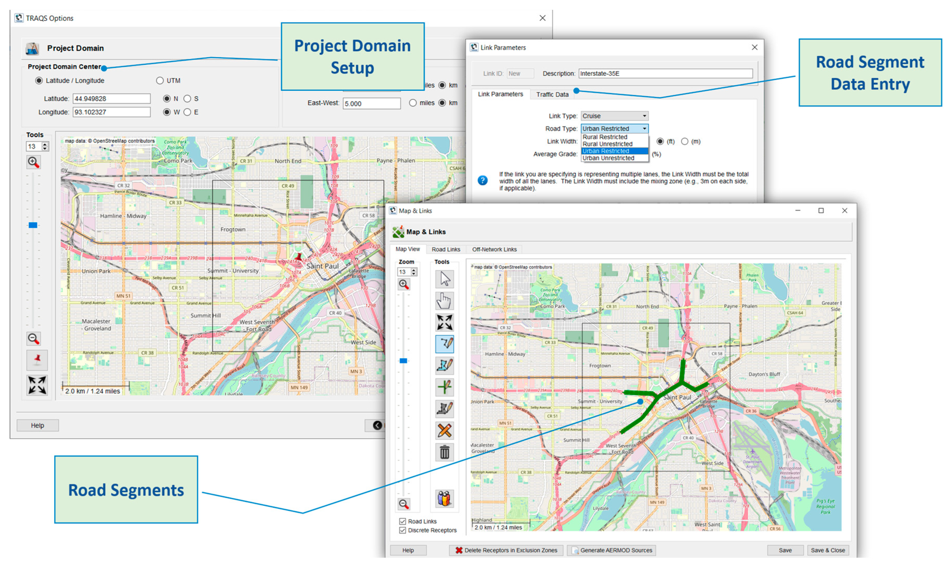
One major impediment in quantifying health impacts from on-road emissions is roadway geometry characterization. MOVES2014b is geospatially unaware and does not require geographic coordinates such as the latitude and longitude to define the road segments in the real world. However, coordinates are required to perform the air dispersion analysis of the MSATs away from the roads towards human receptors. Air dispersion models like AERMOD require precise coordinates to characterize terrain, receptors, and roads, which are considered the emission source rather than the individual vehicles.

The Transportation Air Quality System (TRAQS) [49] is used in this methodology to address roadway geometry characterization. TRAQS addresses the roadway geometry characterization limitation by enabling the user to define the roadway segments within a geographic information system (GIS), automatically saving the precise coordinates in preparation for air dispersion modeling. Figure 2 shows the TRAQS graphical user interface (GUI) and the road segments analyzed in this work.

2.3. Air Dispersion and Deposition Modeling

The air dispersion and deposition modeling subsection is composed of two parts. The first part describes the air dispersion and deposition modeling of MSATs. In the second part, a description of the meteorological files and how they were prepared is presented.

2.3.1. Air Dispersion and Deposition Modeling

Air dispersion modeling is defined as the mathematical description of pollutant transport in the atmosphere. Air dispersion modeling is performed to simulate the transport, diffusion, and deposition of MSATs in the ambient air once emitted by the various emissions processes, such as running exhaust, extended idle exhaust, crankcase running exhaust, or fuel vapor venting.

Air dispersion models are used to predict the downwind concentrations of an emission source, provided the model is fed with all necessary data, such as source parameters like coordinates; physical characteristics like stack height, exit temperature, exit velocity, and diameter; and project-specific data like meteorological conditions, geophysical data layers (e.g., terrain, land use), and receptor information (including sensitive population and ambient air monitor locations).

Air dispersion modeling is needed to:

• Predict air concentrations and deposition on vegetation, land, and water.
• Determine on-road mobile source emission contributions to ambient air quality.
• Better understand how MSATs amplify the deleterious effects of air pollution.
• Aid in ambient air monitoring stations selection, such as identifying target road segments for near-road monitoring.

In this paper, MSATs dispersion and deposition are simulated by an extensively validated Gaussian EPA model, AERMOD (American Meteorological Society (AMS)/United States Environmental Protection Agency (EPA) Regulatory Model). AERMOD is the EPA’s preferred dispersion model for regulatory applications [50]. In this work, a commercialized version of AERMOD called AERMOD View [51] is used to calculate the hourly and annual air concentrations and deposition fluxes resulting from on-road emissions. AERMOD View utilizes EPA’s AERMOD model version 19191.

Our proposed methodology is flexible in incorporating more sophisticated air dispersion models, such as non-steady-state puff models, which simulate three-dimensional complex wind fields and derive meteorology from a combination of upper-air launches and point-based surface observations to estimate ambient air concentrations and deposition.

2.3.2. Meteorological Files

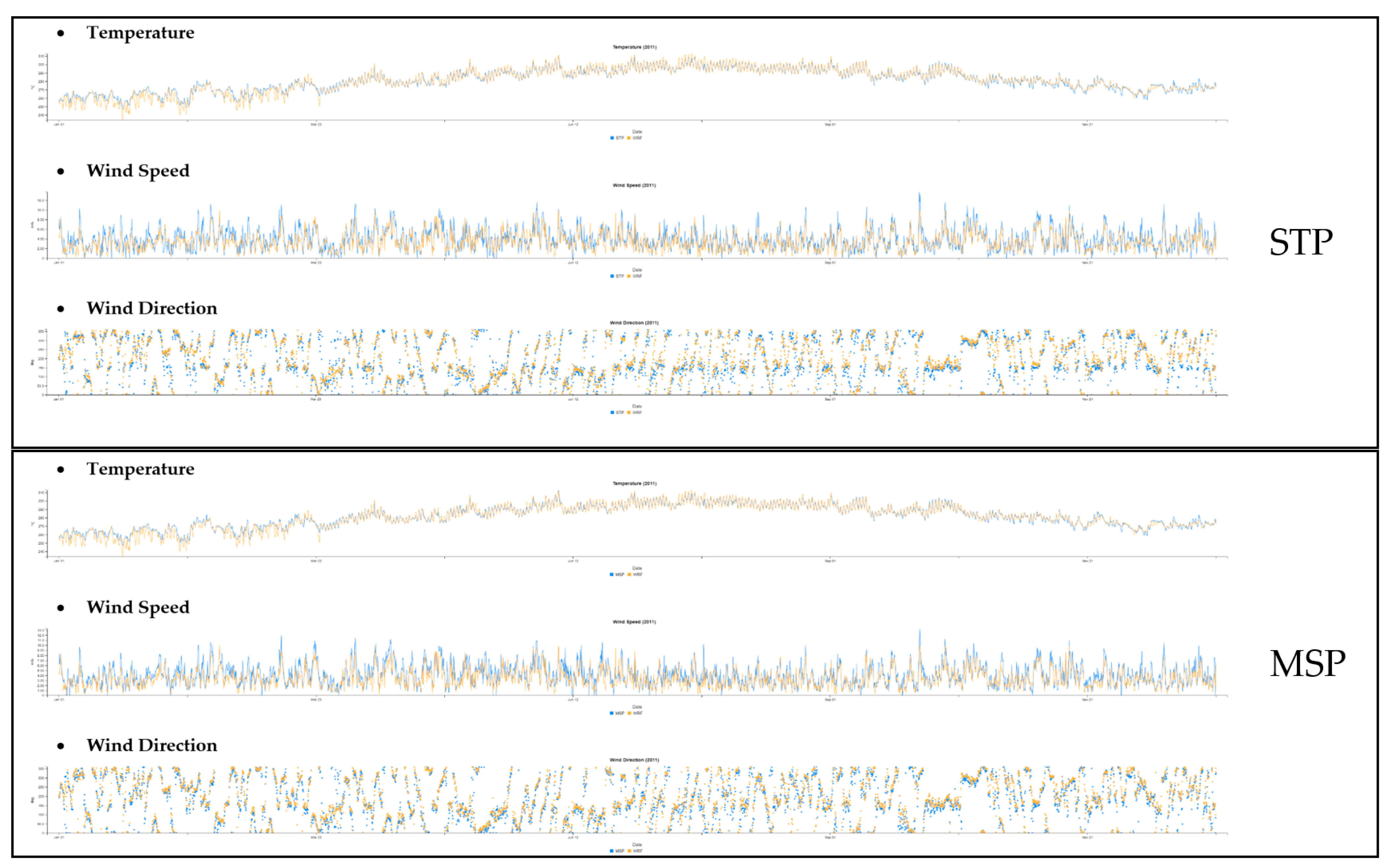
The Weather Research and Forecasting (WRF) model [52] was used to generate the AERMOD meteorological files. WRF is a prognostic meteorology model developed in a collaborative partnership between the U.S. National Center for Atmospheric Research (NCAR), the National Centers for Environmental Prediction (NCEP), the Naval Research Laboratory, and others. The WRF model is a limited-area, non-hydrostatic, terrain-following sigma-coordinate model designed to simulate or predict mesoscale and regional-scale atmospheric circulation.

The air dispersion meteorological files were generated by processing the AERMET-Ready data files output by the Mesoscale Model Interface Program [53] through the most recent version of the U.S. EPA’s AERMET meteorological pre-processor executable (Version 19191). This includes the use of the MMIF-generated AERSURFACE output file for Stage 3 surface characteristics.

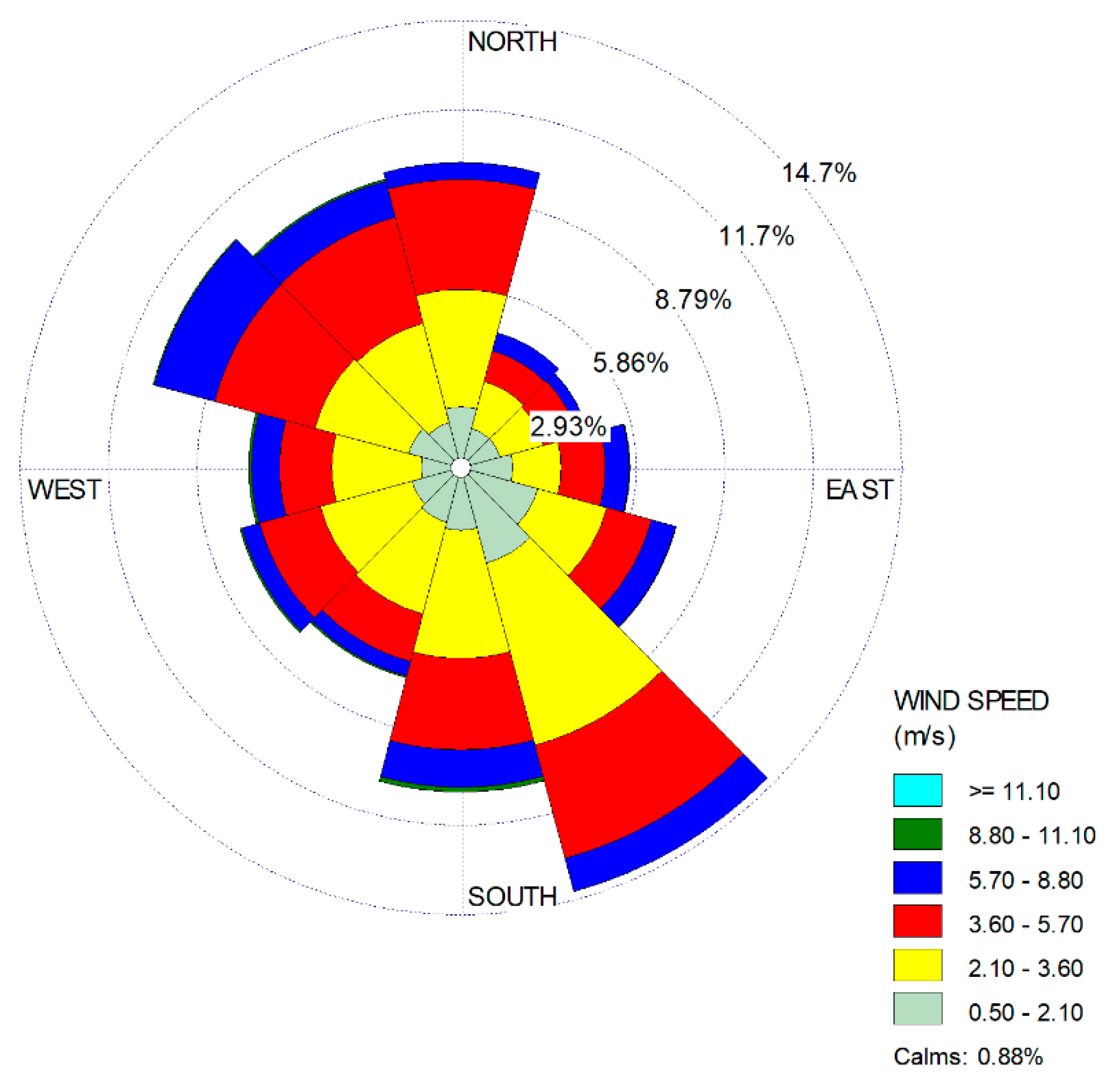
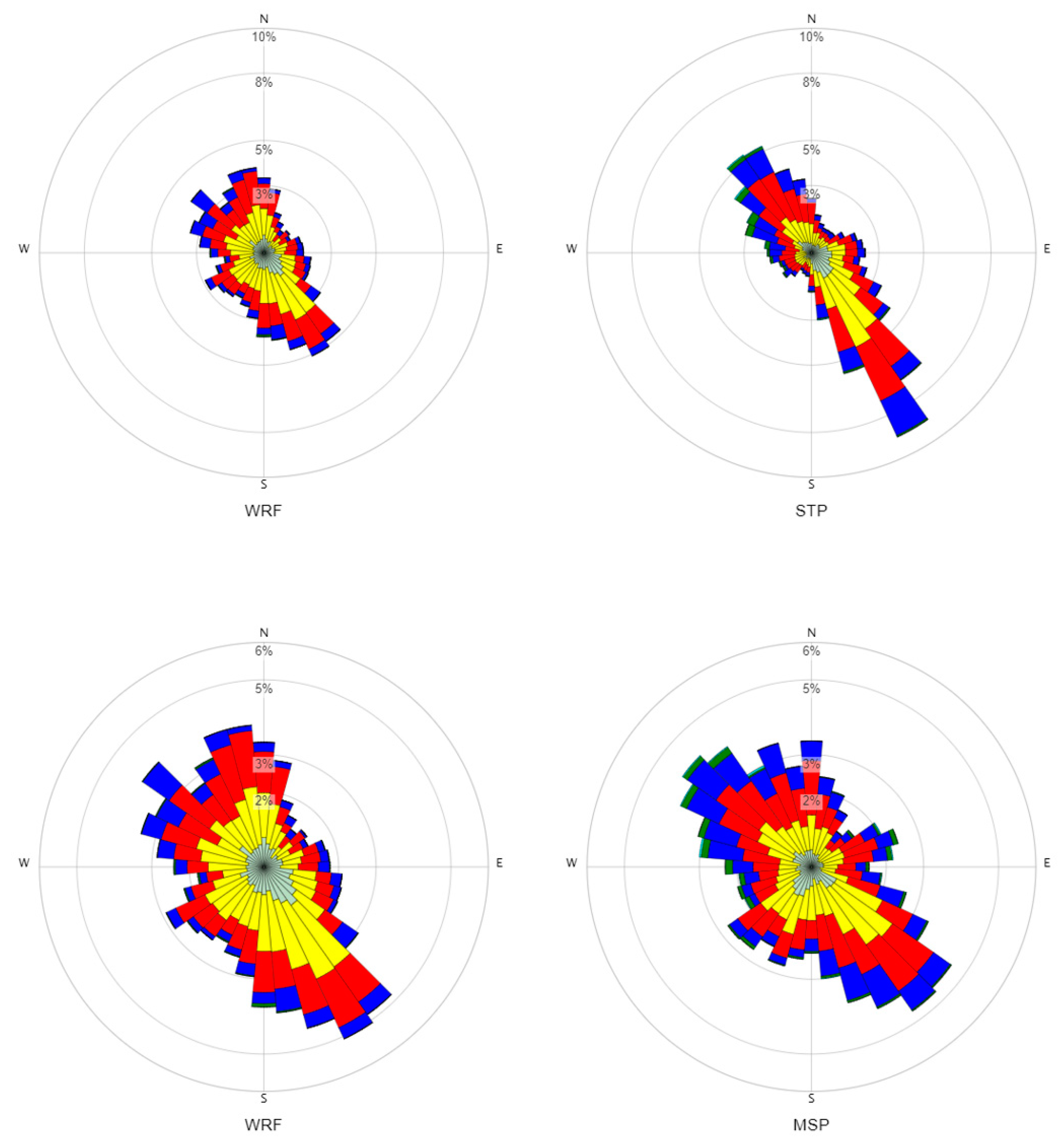
The two generated meteorological data files are: surface data and profile data. The surface data file contains the hourly boundary layer parameter estimates, and the profile data file contains multiple-level observations of wind speed, wind direction, temperature, and standard deviation of the fluctuating wind components. A wind rose for the study area is shown later in the paper in the Case Study subsection.

2.4. Human Health Risk Assessment

Human health risk assessment is the scientific process that estimates the probability that adverse health effects may occur in humans resulting from exposure to environmental stressors, now or in the future. The human health risk assessment process includes the completion of four steps: (1) hazard or stressor identification, (2) exposure assessment, (3) dose-response assessment, and (4) risk characterization. Risk is an estimate of the “chance” that the exposure will cause or contribute to harmful human health effects. Risk characterization is the process whereby human health risk estimates are used to establish the presence or absence of risk and quantification of expected outcomes. In addition, risk characterization strives to identify the key factors contributing to risk in such a way that regulators, risk analysts, or air quality engineers are armed with actionable information to guide decisions regarding what actions, if any, should be taken to mitigate risk. Risk characterization includes calculating the incremental lifetime cancer risks and noncancer hazards by combining the toxicity benchmarks and exposure quantities [54].

Cancer risk is defined as the probability of contracting cancer based on a unique set of exposure and toxicity assumptions throughout a lifetime, which is assumed to be 70 years for this research. For example, a risk of 5.0E-05 is interpreted to mean that an individual has up to a five in 100,000 increased chance of developing cancer during their lifetime from the evaluated exposure. Future research will employ a probabilistic approach for the lifetime variable (e.g., lifetime probability distribution). Noncancer hazard is an estimate of the likelihood that a human will experience noncancer health effects (e.g., neurological, cardiovascular, reproductive, respiratory, etc.) as a result of exposure to MSATs through the scenario-specific exposure pathways and routes. A hazard is calculated as a ratio of the receptor’s potential exposure relative to a standard exposure level such as a reference dose or reference concentration.

There are two primary hazard classifications based on the length of the exposure duration: acute for short term, and chronic for long term.

The multi-pathway and cumulative human health risk assessment in this paper was performed following the U.S. EPA 2005 Final Human Health Risk Assessment Protocol (HHRAP) [26]. The HHRAP provides guidance for completing a human health risk assessment study from modeled air concentrations and deposition fluxes. HHRAP was developed for evaluating human health risks from hazardous waste combustion facilities such as incineration plants or energy generation plants. This research (utilizing source characterization for mobile sources) extended (added utilizing source characterization for mobile sources; adapted to mobile sources) HHRAP in evaluating health risks associated with exposure to MSATs. The chronic and acute dose-response values were obtained from the following sources: (1) U.S. EPA’s Integrated Risk Information System [55], (2) California’s EPA (CalEPA) chemical database [56], (3) CDC’s Agency for Toxic Substances and Disease Registry Toxic Substances Portal [57]. For MSATs with multiple dose-response values from the above sources, the more conservative value was selected.

To quantify the potential health risks associated with exposure to MSATs, target levels are commonly established by the regulatory agency to gauge the magnitude of risk, which in turn influences decisions regarding the management of risk. The HHRAP does not define target risk levels, as this responsibility is left to local and state regulatory agencies, who are better equipped to consider other factors such as background concentrations. However, the U.S. EPA, through its Region 6 Office [58], has established target risk levels within the Agency, which range as follows: (1) for carcinogenic risks, a low and likely to be a negligible risk is described as an incremental lifetime cancer risk of 1.0E-06 to less than 1.0E-05; (2) a potentially elevated risk is an incremental lifetime cancer risk greater than 1.0E-04; (3) for noncancer hazards, a low and likely to be a negligible risk is defined as being a hazard quotient ranging between 0 and 0.25. In this work, the following target levels are used to interpret the magnitude of cancer risks and noncancer hazards: a cancer risk not to exceed a target risk level of 1.0E-05, and a hazard quotient not to exceed a target risk level of 0.25.

The target risk levels are not a discrete indicator of observed harmful effects. If the modeled risk values fall within the accepted target risk levels, it might be concluded, without further analysis, that a proposed project does not present an unacceptable risk. A risk calculation that exceeds the target values triggers further consideration of the underlying scientific basis and uncertainties associated with the risk calculation.

The general equations used to calculate the cancer risk and noncancer risk in this work are:

$$\mathrm{Cancer} \mathrm{Risk} = \mathrm{dose} \times \mathrm{toxicity}$$

(1)

$$\mathrm{Noncancer} \mathrm{Risk} =\frac{\mathrm{average} \mathrm{daily} \mathrm{dose}}{\mathrm{reference} \mathrm{dose}}$$

(2)

$${\mathrm{Noncancer} \mathrm{Risk}}_{\mathrm{inh}}=\frac{\mathrm{exposure} \mathrm{air} \mathrm{concentration}}{\mathrm{reference} \mathrm{concentration}}$$

(3)

$${\mathrm{Acute} \mathrm{Hazard} \mathrm{Quotient}}_{\mathrm{inh} }=\frac{\mathrm{acute} \mathrm{air} \mathrm{concentration}}{\mathrm{acute} \mathrm{inhalation} \mathrm{exposure} \mathrm{criteria}}$$

(4)

Equation (2) is used to calculate the noncancer risk from oral exposure, whereas Equation (3) evaluates the noncancer risk from inhalation exposure. Equation (4) is used to calculate the acute (short-term) inhalation hazard quotient.

2.4.1. Cumulative Risk

Humans may be exposed to multiple carcinogenic air toxics via a single exposure pathway such as inhalation. The total cancer risk for a single pathway is calculated from the sum of cancer risks for each Mobile Source Air Toxic (MSAT) (e.g., benzene, formaldehyde, and benzo(a)pyrene). In addition, exposure may come via multiple pathways (e.g., inhalation, produce, animal tissues, water); therefore, the cumulative cancer risk is calculated from the sum of total cancer risks for each exposure pathway.

2.4.2. Risk Modeling

Due to the complex nature of MSATs fate and transport in different media such as air, water, soil, and atmospheric deposition, more than 78 fate, transport, and exposure equations are used to compute media concentrations, potential cancer risk, and noncancer health effects. Many of these equations are non-linear, such as the calculation of the cumulative soil concentration, calculation of MSATs loss due to runoff, or the calculation of aboveground produce concentration due to direct deposition of particle-phase MSATs such as benzo(a)pyrene or diesel particulate matter.

A hybrid modeling approach was used to calculate the cancer and noncancer risks and cumulative risk. The hybrid model consists of a computer program known as IRAP-h View [59] and a Python program written by the authors. IRAP-h View follows the methodologies published in the Human Health Risk Assessment Protocol (HHRAP). IRAP-h View, also known as the risk engine or risk modeling platform in this work, was used to calculate the cancer and noncancer risks encapsulating all the guidance and procedures contained in HHRAP. The cumulative risk was calculated using the Python code.

In addition to modeled ground level air concentrations, our proposed methodology is flexible in utilizing in situ measured concentrations from near-road monitoring and air monitoring networks to estimate risk resulting from exposure to MSATs through the inhalation exposure pathway.

This paper fills gaps in the mobile emissions health impact literature, as described below:

• Mobile Emissions Inventory Data Quality—This work generates the on-road vehicle emissions inventory using a state-of-the-science simulator instead of using outdated emission factors. Additionally, the methodology presented in the paper is flexible in incorporating spatiotemporal considerations to improve the characterization of emissions and health impacts.
• Spatial Accuracy—The Vehicle Emission Simulator (MOVES) lacks spatial information. To fill this gap, the present work geospatially links the emissions results to air dispersion and deposition models, air toxics fate and transport analysis, and a risk modeling platform to estimate the impacts of MSATs on humans.
• Allocation of Source Impacts—Previous work accounted for a lumped air concentration and could not apportion sources to specific human impacts. This work conducts a multi-pathway fate-and-transport analysis of MSATs, source by source. This allows allocating the contribution of each source’s deleterious effects from on-road mobile sources, revealing the full extent of exposure to MSATs.

3. Results

3.1. Case Study

A case study for high-traffic roadway segments located in the city of Saint Paul in the U.S. state of Minnesota is presented. The roadway segments are within the Interstate-35E and Interstate-94 and US-10 in Saint Paul junction, and the study area is in Ramsey County. Figure 3 shows the location of the high-traffic roadway.

This study area was selected because it contains roadway segments that rank amongst the highest annual average daily traffic (AADT) in Ramsey County [60] and because there is a near-road monitoring site (Saint Paul—Ramsey Health Center with AQS Site ID: 27-123-0868) within the study area. The Saint Paul—Ramsey Health Center monitoring site is located at 44°57′2.50″ N, 93°5′54.60″ W and was chosen to be the project center.

Table 2. Project Center in Saint Paul Annual Average Daily Traffic (AADT).

Year	AADT
2011	183,000
2017	197,000
2018	203,000
2019	203,000
2020	160,000

shows the AADT at the nearest point to the project center for the following years: 2011, 2017, 2018, 2019, and 2020.

The datasets used for the models’ input and validation in this case study are from 2011. The 2017, 2018, and 2019 AADT were included in Table 2 to demonstrate the upward trend of vehicle volume growth from 2011. However, the AADT in 2020 dropped from 2019 due to the COVID-19 pandemic.

The following subsubsections contain information on the air dispersion model setup, meteorological data for the study area, sensitive receptors, developed exposure scenarios, and target risk levels.

3.1.1. Air Dispersion Model Setup

The high-traffic roadway segments were modeled as a series of area sources in AERMOD View. Area sources were selected because they are one of the preferred ways to represent vehicle emissions based on guidance from the EPA [61,62], and these types of sources create a uniform emission characterization of a roadway segment. In addition, the area source algorithm does not contain distance restrictions for model calculations like point and volume sources.

Ground-level concentrations of the MSATs were modeled using AERMOD with its non-default regulatory model options. These options include the use of elevated terrain, Fast Area Sources (FASTAREA), optimized Area Source Plume Depletion (AREADPLT), and the use of processing routines to handle calm and missing meteorological data.

The annual and 1-h averaging times were selected, and the following control pathway specifications were included: concentration, dry deposition, wet deposition, and total deposition. In addition, the dry and wet depletion options were selected to account for plume depletion due to dry and wet removal mechanisms.

The air dispersion modeling was conducted using the unit emission rate concept, where the entire area source is emitting at a rate of 1 g per second divided by the source area. This modeling approach eliminates multiple air dispersion modeling runs for the vast number of MSATs. Scaling of the unitized concentrations by the appropriate MSATs emission rate is applied in the risk modeling platform.

3.1.2. Prognostic Weather Setup

The Weather Research and Forecasting (WRF) model was used to generate the air dispersion meteorological files for the project area for 2011. A 4-km refined grid cell resolution was selected to depict the meteorological characteristics of the project area adequately. The wind rose, employing WRPLOT View [63], for the project center is shown in Figure 4.

Following the successful execution of WRF, three meteorological variables (i.e., wind direction, wind speed, and temperature) were extracted and analyzed against measurements from two meteorological stations (Saint Paul Downtown Airport and Minneapolis-Saint Paul International Airport), both located within 13 km of the WRF center point. Operational analysis of these variables was conducted following standard recommendations on statistical analysis procedures for validating meteorological model performance. The metrics used to evaluate the model performance are bias, mean absolute error, root mean square error, and index of agreement. These metrics were compared against established model performance benchmarks for meteorological models [64]. For example, common benchmarks for the index of agreement include a value greater than or equal to 0.8 [65].

The WRF data were compared to surface weather observations at two meteorological stations, showing good agreement, while statistical error measurements indicated satisfactory agreement between the WRF model and observations. Based on these comparisons, it is suggested that the WRF model adequately represents the weather conditions for Saint Paul, Minnesota, and its surrounding areas at the centermost grid cell. A detailed description of the WRF validation study can be found in Appendix A.

In 2011, the prevailing winds blew from the southeast 15% of the time, with an average speed of 3.41 m/s. Statistical analysis of meteorological data such as frequency distributions and count is important in understanding the probability of downwind impacts. In addition, wind speed and direction variability heavily influence the transport of traffic-related air toxics and thus exposure. Studies found that the average concentrations of MSATs in a neighborhood decreased as wind speeds increased. The decrease in concentrations is mainly due to horizontal dilution and vertical dilution, which is a function of mixing layer height [66,67,68,69].

3.1.3. Sensitive Receptors

Sensitive receptors are locations where people are more susceptible to adverse effects of exposure to mobile source air toxics (e.g., schools, hospitals, places of worship, etc.). Three sensitive receptors were included in the multi-pathway human health risk assessment, and the names and locations of these receptors are summarized in

Table 3. Assessed Sensitive Receptor Locations.

Sensitive Receptor	Sensitive Receptor Name	Latitude and Longitude
Receptor 1	Saint Paul—Ramsey Health Center	44°57′2.50″ N, 93°5′54.60″ W
Receptor 2	Anderson Office Building	44°57′3.90″ N, 93°5′48.59″ W
Receptor 3	Minnesota State Capitol	44°57′18.71″ N, 93°6′8.21″ W

.

The criteria to identify and set up these sensitive receptors included the following steps:

• Identify the project grid nodes with the maximum modeled values for each air parameter within a defined area. These air parameters include unitized hourly air concentrations from vapor, particle, and particle-bound phases and unitized annual average air concentrations from vapor, particle, and particle-bound phases.
• Ignore grid nodes located in the middle of the roadway, as evaluating risk at locations where people are exposed intermittently is not the focus of this work.
• Select the applicable exposure scenarios (discussed below).

3.1.4. Multi-Pathway Exposure Scenarios

The multi-pathway human health risk assessment was conducted for the following four exposure scenarios: Farmer Adult, Farmer Child, Urban Resident Adult, and Urban Resident Child. For each of the three sensitive receptors, the evaluated exposure pathways are summarized in

Table 4. Evaluated Exposure Pathways.

Exposure Pathways	Applicable Exposure Scenario
Direct Inhalation of Vapors and Particles	Urban Residents and Farmers
Incidental Ingestion of Soil	Urban Residents and Farmers
Ingestion of Drinking Water from Surface Water Sources	Urban Residents and Farmers
Ingestion of Homegrown Produce	Urban Residents and Farmers
Ingestion of Homegrown Beef	Applies only to Farmers
Ingestion of Milk from Homegrown Cows	Applies only to Farmers
Ingestion of Homegrown Chicken	Urban Residents and Farmers
Ingestion of Eggs from Homegrown Chicken	Urban Residents and Farmers
Ingestion of Homegrown Pork	Applies only to Farmers

. Future work will incorporate additional exposure scenarios such as Fisher Adult and Fisher Child and unique scenarios such as hunter (e.g., deer meat consumption).

This subsubsection describes a few key exposure parameters, including duration, frequency, averaging time, and rates of ingestion and inhalation. These factors are evaluated in human health risk assessments to quantify exposure through different exposure routes such as ingestion, inhalation, and dermal exposure.

Exposure duration is the length of time that a receptor (individual or population) is exposed to the MSATs being evaluated. Exposure frequency is defined as the frequency with which the exposure occurs. This exposure parameter is provided in number of days per year. A typical conservative value of 350 days per year is used based on the protective assumption that a receptor (e.g., an individual) spends a maximum of two weeks away from the exposure source. The averaging time is the period over which exposure is averaged, and this parameter varies with the type of MSATs. For example, for carcinogenic MSATs, the averaging time equals 25,550 days (cumulative intake is prorated over a lifetime of 70 years). In contrast, the averaging time for noncancerous MSATs equals the exposure duration multiplied by 365 days.

The inhalation rate is described as the amount of air inhaled over a specified period. This value should be representative of the population being evaluated when conducting human health risk assessments. An inhalation rate of 0.83 m³/h is recommended for an adult, and 0.3 m³/h for a child [26]. These values correspond to 20 m³/day and 7 m³/day, respectively.

The ingestion rate is defined as the amount of water, food (including produce, fish, fruits, meat, etc.), or soil containing the MSATs that a receptor (e.g., individual or population) ingests during a specified period. The ingestion rate parameter is expressed in units of mass per unit time. As mentioned above, a representative ingestion rate value should be used when estimating human health risk associated with exposure to MSATs.

3.1.5. Target Risk Levels

The target risk levels for evaluating exposure to MSATs are narrowed to increase the level of conservatism and to account for exposure to the study area’s background concentrations and account for different lifestyles. These targets are used in this paper to interpret the magnitude of cancer risks and noncancer health effects. The target risk levels are summarized in

Table 5. Target Risk Levels.

Description	Value	Normalized Value
Cancer Risk Threshold	1.0E-05	1.0E-05/1.0E-05 = 1
Hazard Quotient Threshold	0.25	0.25/0.25 = 1

.

3.2. Air Dispersion and Deposition Model Results

In this subsection, we begin by presenting the air dispersion and deposition model results, including the ground-level air dispersion patterns (contour plots) for each MSAT and the deposition term for each MSAT at the three sensitive receptors.

The annual average concentrations generated by the air dispersion simulation were used to evaluate potential adverse health impacts from chronic exposure to MSATs. In addition, the generated maximum 1-h concentrations were used to evaluate the potential for adverse health effects from acute exposure. The contours shown in this subsection were generated from the air dispersion model’s maximum hourly and annual average results. The concentration values presented in this subsection symbolize the unitized values; these values are expressed in µg-s/g-m³.

3.2.1. Benzene

The fraction of benzene’s air concentration in the vapor phase (F_v) equals 1 [26]; therefore, only the vapor phase was modeled. Figure 5 shows the benzene unitized maximum hourly air concentrations (in µg-s/g-m³) from the vapor phase contour plot, and Figure 6 shows the unitized annual average air concentrations (in µg-s/g-m³) from the vapor phase.

The generated contours are based on the distribution of the modeled results, and the modeled sources are represented by the red triangles in Figure 5 and Figure 6.

In Figure 5, the maximum concentration observed within the modeled domain is 289.7 µg-s/g-m³. Areas of high concentration values are clustered around the project’s center, and the maximum value’s location is 44°56′59.4′′ N, 93°6′8.35′′ W (491,928.63 m E, 4,977,382.64 m N, Zone 15 in UTM Coordinate System).

In Figure 6, the annual maximum concentration value dropped to 4.1 µg-s/g-m³ due to the annual averaging. The annual averaging is the arithmetic mean of the 8760 hourly concentrations minus calm and missing hours. The unitized benzene maximum concentration (in µg-s/g-m³) values and their locations are shown in

Table 6. Benzene Maximum Concentration Values and their Respective Locations.

Air Parameter	Maximum (Max) Concentration	Location of Max in Degrees and UTM
Unitized hourly air concentration from vapor phase	289.7 µg-s/g-m3	44°56′59.4″ N, 93°6′8.35″ W (491,928.63 m E, 4,977,382.64 m N, Zone 15)
Unitized annual average air concentration from vapor phase	4.1 µg-s/g-m3

.

3.2.2. Formaldehyde

Like benzene, the fraction of formaldehyde’s air concentration in the vapor phase equals 1 [26]; therefore, formaldehyde is assumed to only occur in the vapor phase. Figure 7 shows the formaldehyde unitized maximum hourly air concentrations from the vapor phase contour plot.

In Figure 7, the maximum air concentration value is 271.8 µg-s/g-m³. Similar to benzene, high concentrations were located near the project’s center. The unitized annual average air concentrations from the vapor phase ground-level air dispersion pattern are shown in Figure 8.

A summary of the unitized formaldehyde maximum concentration values and their locations is provided in

Table 7. Formaldehyde Maximum Concentration Values and their Respective Locations.

Air Parameter	Maximum (Max) Concentration	Location of Max in Degrees and UTM
Unitized hourly air concentration from vapor phase	271.8 µg-s/g-m3	44°56′59.4″ N, 93°6′8.35″ W (491,928.63 m E, 4,977,382.64 m N, Zone 15)
Unitized annual average air concentration from vapor phase	4.07 µg-s/g-m3

.

The observed similarity in the shapes of the ground-level air dispersion patterns (contour plots) presented in Figure 5, Figure 6, Figure 7 and Figure 8 is explained by the likeness of the benzene and formaldehyde emission rates values. The slight differences in the concentration results presented in Table 6 and Table 7 are based solely on the differences in gas deposition input parameters for benzene and formaldehyde. The gas deposition parameters are pollutant diffusivity in air, pollutant diffusivity in water, cuticular resistance, and Henry’s law constant.

3.2.3. Benzo(a)pyrene (BaP)

The fraction of BaP’s air concentration in the vapor phase (Fv) is 0.294, and the balance (0.706) is emitted as condensed in a particle-bound portion [26]. Particle-bound modeling requires the provision of particle size distributions for particles originating from on-road sources.

The fate and transport of these particles is determined by the size of the particle, and larger particles deposit closer to the source, whereas smaller particles remain suspended in the air for prolonged periods [70]. In other words, BaP can be transported over long distances and deposited farther away from the source [71].

Figure 9 shows the BaP unitized maximum hourly air concentrations from the vapor phase contour plot; the unitized maximum hourly air concentrations from the particle-bound phase contour plot are shown in Figure 10.

The calculated unitized maximum hourly air concentration from the vapor phase value is 263.7 µg-s/g-m³, and the unitized maximum hourly air concentration value for the particle-bound phase is 283.7 µg-s/g-m³. Both maximum hourly concentrations occurred near the on-road emissions sources.

Figure 11 and Figure 12 show the unitized annual average air concentrations from the vapor and particle-bound phases contour plots, respectively.

The contour plots in both Figure 11 and Figure 12 show that the maximums have decreased as compared to the hourly air concentrations. The unitized maximum concentration values and their respective locations are shown in

Table 8. Benzo(a)pyrene Maximum Concentration Values and their Respective Locations.

Air Parameter	Maximum (Max) Concentration	Location of Max in Degrees and UTM
Unitized hourly air concentration from vapor phase	263.7 µg-s/g-m3	44°56′59.38″ N, 93°6′8.38″ W (491,927.97 m E, 4,977,382.02 m N, Zone 15)
Unitized hourly air concentration from particle bound	283.7 µg-s/g-m3
Unitized annual average air concentration from vapor phase	4.01 µg-s/g-m3
Unitized annual average air concentration from particle bound	4.06 µg-s/g-m3

.

3.2.4. Deposition Term

The deposition term represents the rate at which particles and vapor phase MSATs are directly deposited from air to soil, water, and above-ground produce. The deposition term is the predominant driver of MSATs concentrations in the indirect exposure pathways. A summary of the results at the three sensitive receptors is shown in

Table 9. Deposition Term Calculated Values at the Three Receptor Locations.

	Deposition Term [Milligram MSATs/kg Soil]
Sensitive Receptor	Benzene	Formaldehyde	Benzo(a)pyrene
Saint Paul—Ramsey Health Center	1.60E-03	1.75E-01	4.30E-04
Anderson Office Building	6.32E-04	7.48E-02	1.84E-04
Minnesota State Capitol	7.49E-05	1.24E-02	2.59E-05

.

The MSATs deposition rates per unit area of soil are calculated from the unitized annual average dry and wet deposition fluxes from the vapor phase. The dry and wet deposition fluxes are calculated from the ambient air quality modeling conducted for benzene, formaldehyde, and benzo(a)pyrene.

The highest deposition term value (italicized) was calculated at the Saint Paul—Ramsey Health Center for benzo(a)pyrene. The maximum deposition term value associated with BaP comes as no surprise due to the physicochemical properties of this aromatic hydrocarbon [71,72], particle size distribution, and the phases it is emitted in (e.g., vapor phase and particle-bound phase).

3.3. Risk Results

This subsection summarizes the results of the comprehensive multi-pathway human health risk assessment, and the following results (standard and normalized) are included:

• Total individual (i.e., MSATs-specific) cancer risks and noncancer hazards.
• Acute Hazard Quotient.
• Cumulative excess lifetime cancer risks (ELCRs) and chronic noncancer hazards.

The normalized risk values were computed by dividing the calculated risk value, cancer or noncancer, by the respective target risk level (e.g., cancer values were divided by 1.0E-05, and hazard values were divided by 0.25). Italicized risk values indicate a value exceeding the Target Risk Levels shown in Table 5.

3.3.1. Total Individual Cancer Risks and Noncancer Hazards

Table 10. Total Individual Benzene Cancer Risks and Noncancer Hazards.

Saint Paul—Ramsey Health Center
Risk	Urban Resident Adult	Urban Resident Child	Farmer Adult	Farmer Child
Cancer	5.30E-07	1.06E-07	7.06E-07	1.06E-07
Hazard	5.28E-03	5.28E-03	5.28E-03	5.28E-03
Normalized Results (Cancer Values Divided by 1.0E-05, Hazard Values Divided by 0.25)
Risk	Urban Resident Adult	Urban Resident Child	Farmer Adult	Farmer Child
Cancer	5.30E-02	1.06E-02	7.06E-02	1.06E-02
Hazard	2.11E-02	2.11E-02	2.11E-02	2.11E-02
Anderson Office Building
Risk	Urban Resident Adult	Urban Resident Child	Farmer Adult	Farmer Child
Cancer	2.37E-07	4.74E-08	3.16E-07	4.74E-08
Hazard	2.37E-03	2.37E-03	2.37E-03	2.37E-03
Normalized Results
Risk	Urban Resident Adult	Urban Resident Child	Farmer Adult	Farmer Child
Cancer	2.37E-02	4.74E-03	3.16E-02	4.74E-03
Hazard	9.46E-03	9.46E-03	9.46E-03	9.46E-03
Minnesota State Capitol
Risk	Urban Resident Adult	Urban Resident Child	Farmer Adult	Farmer Child
Cancer	3.81E-08	7.63E-09	5.08E-08	7.63E-09
Hazard	3.80E-04	3.80E-04	3.80E-04	3.80E-04
Normalized Results
Risk	Urban Resident Adult	Urban Resident Child	Farmer Adult	Farmer Child
Cancer	3.81E-03	7.63E-04	5.08E-03	7.63E-04
Hazard	1.52E-03	1.52E-03	1.52E-03	1.52E-03

,

Table 11. Total Individual Formaldehyde Cancer Risks and Noncancer Hazards.

Saint Paul—Ramsey Health Center
Risk	Urban Resident Adult	Urban Resident Child	Farmer Adult	Farmer Child
Cancer	9.43E-07	1.89E-07	1.26E-06	1.89E-07
Hazard	1.75E-02	1.76E-02	1.75E-02	1.77E-02
Normalized Results (Cancer Values Divided by 1.0E-05, Hazard Values Divided by 0.25)
Risk	Urban Resident Adult	Urban Resident Child	Farmer Adult	Farmer Child
Cancer	9.43E-02	1.89E-02	1.26E-01	1.89E-02
Hazard	6.99E-02	7.05E-02	7.00E-02	7.08E-02
Anderson Office Building
Risk	Urban Resident Adult	Urban Resident Child	Farmer Adult	Farmer Child
Cancer	4.21E-07	8.42E-08	5.61E-07	8.42E-08
Hazard	7.79E-03	7.86E-03	7.81E-03	7.89E-03
Normalized Results
Risk	Urban Resident Adult	Urban Resident Child	Farmer Adult	Farmer Child
Cancer	4.21E-02	8.42E-03	5.61E-02	8.42E-03
Hazard	3.12E-02	3.14E-02	3.12E-02	3.16E-02
Minnesota State Capitol
Risk	Urban Resident Adult	Urban Resident Child	Farmer Adult	Farmer Child
Cancer	6.73E-08	1.35E-08	8.97E-08	1.35E-08
Hazard	1.25E-03	1.26E-03	1.25E-03	1.26E-03
Normalized Results
Risk	Urban Resident Adult	Urban Resident Child	Farmer Adult	Farmer Child
Cancer	6.73E-03	1.35E-03	8.97E-03	1.35E-03
Hazard	4.99E-03	5.03E-03	5.00E-03	5.05E-03

and

Table 12. Total Individual Benzo(a)pyrene Cancer Risks and Noncancer Hazards.

Saint Paul—Ramsey Health Center
Risk	Urban Resident Adult	Urban Resident Child	Farmer Adult	Farmer Child
Cancer	1.86E-07	8.41E-08	4.59E-05	9.87E-06
Hazard	7.18E-02	7.21E-02	1.08E-01	1.24E-01
Normalized Results (Cancer Values Divided by 1.0E-05, Hazard Values Divided by 0.25)
Risk	Urban Resident Adult	Urban Resident Child	Farmer Adult	Farmer Child
Cancer	1.86E-02	8.41E-03	4.59E+00	9.87E-01
Hazard	2.87E-01	2.88E-01	4.34E-01	4.97E-01
Anderson Office Building
Risk	Urban Resident Adult	Urban Resident Child	Farmer Adult	Farmer Child
Cancer	8.00E-08	3.61E-08	2.02E-05	4.34E-06
Hazard	3.20E-02	3.21E-02	4.81E-02	5.50E-02
Normalized Results
Risk	Urban Resident Adult	Urban Resident Child	Farmer Adult	Farmer Child
Cancer	8.00E-03	3.61E-03	2.02E+00	4.34E-01
Hazard	1.28E-01	1.28E-01	1.92E-01	2.20E-01
Minnesota State Capitol
Risk	Urban Resident Adult	Urban Resident Child	Farmer Adult	Farmer Child
Cancer	1.16E-08	5.16E-09	3.12E-06	6.70E-07
Hazard	5.11E-03	5.12E-03	7.59E-03	8.67E-03
Normalized Results
Risk	Urban Resident Adult	Urban Resident Child	Farmer Adult	Farmer Child
Cancer	1.16E-03	5.16E-04	3.12E-01	6.70E-02
Hazard	2.04E-02	2.05E-02	3.04E-02	3.47E-02

summarize the total individual cancer risks and noncancer hazards for each MSAT (e.g., benzene, formaldehyde, and benzo(a)pyrene) across all pathways for four exposure scenarios at three different locations (sensitive receptors) within the Interstate-35E and Interstate-94 and US-10 in the Saint Paul junction study area. Italicized risk values indicate a value exceeding the Target Risk Levels.

From the three analyzed MSATs, the calculated human health risks resulting from exposure to benzene and formaldehyde fall below the target level of 1.0E-05 for cancer and 0.25 for noncancer hazard risks; however, the calculated risk from benzo(a)pyrene exposure exceeds the target risk level for cancer. From Table 12, the calculated cancer risk for the Farmer Adult scenario at the Saint Paul—Ramsey Health Center receptor exceeds the published target levels, with a risk value of 4.59E-05, which is equal to “45.9 in 1 million people”. Similarly, the calculated cancer risk for the Farmer Adult scenario at the Anderson Office Building receptor exceeded the target levels. The calculated risk value at the Anderson Office Building receptor is 2.02E-05, which is equal to “20.2 in 1 million people”. The elevated cancer risk results at the Saint Paul—Ramsey Health Center were expected because that location had the maximum calculated air concentration and the maximum deposition term value. These values are 1.49E-04 µg/m³ and 4.30E-04 milligram benzo(a)pyrene per kg soil, respectively.

3.3.2. Acute Hazard Quotient-Inhalation (AHQ_inh)

Table 13. Maximum Hourly Air Concentrations and Acute Hazard Quotient AHQ_inh Results.

Saint Paul—Ramsey Health Center
Mobile Source Air Toxics (MSATs)	Maximum Hourly Air Concentration (µg/m3)	AHQinh	AHQinh (Normalized)
Benzene	7.96E+00	6.12E-03	2.45E-02
Formaldehyde	8.25E+00	8.77E-02	3.51E-01
Benzo(a)pyrene	7.04E-03	1.17E-05	4.69E-05
Anderson Office Building
Mobile Source Air Toxics (MSATs)	Maximum Hourly Air Concentration (µg/m3)	AHQinh	AHQinh (Normalized)
Benzene	8.99E+00	6.91E-03	2.76E-02
Formaldehyde	9.33E+00	9.92E-02	3.97E-01
Benzo(a)pyrene	7.98E-03	1.33E-05	5.32E-05
Minnesota State Capitol
Mobile Source Air Toxics (MSATs)	Maximum Hourly Air Concentration (µg/m3)	AHQinh	AHQinh (Normalized)
Benzene	3.04E+00	2.34E-03	9.37E-03
Formaldehyde	3.05E+00	3.25E-02	1.30E-01
Benzo(a)pyrene	2.66E-03	4.44E-06	1.77E-05

summarizes the acute hazard quotient-inhalation (AHQ_inh) at the study area’s three different sensitive receptors. The acute inhalation risk is evaluated by comparing the maximum 1-h (acute) air concentrations estimated by the air dispersion model to the acute inhalation exposure criteria (AIEC). The calculated acute hazard quotients for the three analyzed MSATs, which are used to evaluate short-term inhalation exposures to estimate noncancer health effects, all fall within the range of target levels. Therefore, actual short-term exposure to benzene, formaldehyde, or benzo(a)pyrene resulting from mobile emissions is believed to be well within acceptable risk levels. Table 13 summarizes the maximum hourly air concentrations, the respective acute hazard quotient at the three sensitive receptor locations, and the normalized acute hazard quotient.

3.3.3. Cumulative Excess Lifetime Cancer Risks and Chronic Noncancer Hazards

The normalized cumulative excess lifetime cancer risks (ELCRs) and noncancer hazards across all pathways for four exposure scenarios at three sensitive receptors are presented in

Table 14. Normalized Cumulative Excess Lifetime Cancer Risks and Chronic Noncancer Hazards.

Excess Lifetime Cancer Risks (ELCRs) (Across All Pathways)
Sensitive Receptor/Exposure Scenarios	Urban Resident		Farmer
	Adult	Child	Adult	Child
Saint Paul—Ramsey Health Center	1.66E-01	3.79E-02	4.79E+00	1.02E+00
Anderson Office Building	7.38E-02	1.68E-02	2.11E+00	4.47E-01
Minnesota State Capitol	1.17E-02	2.63E-03	3.26E-01	6.91E-02
Noncancer Hazard Indices (Across All Pathways)
Sensitive Receptor/Exposure Scenarios	Urban Resident		Farmer
	Adult	Child	Adult	Child
Saint Paul—Ramsey Health Center	3.78E-01	3.80E-01	5.25E-01	5.89E-01
Anderson Office Building	1.69E-01	1.69E-01	2.33E-01	2.61E-01
Minnesota State Capitol	2.69E-02	2.70E-02	3.69E-02	4.12E-02

. The estimated cumulative ELCRs were calculated by summing up the total individual (i.e., MSATs-specific) cancer risks for each exposure pathway and scenario.

Likewise, the cumulative noncancer hazards were calculated by adding the MSATs individual hazard indices. The cited method for noncancer risk is conservative, and a non-conservative approach would be to separate each hazard index by its toxic endpoint and have separate noncancer hazards for each.

The ELCRs for the Farmer Adult and Farmer Child scenarios are above the cancer risk threshold at the Saint Paul—Ramsey Health Center. Similarly, the Farmer Adult scenario ELCRs exceed the U.S. EPA’s acceptable range at the Anderson Office Building. However, all the other exposure scenarios are within the acceptable risk levels. The potential for adverse noncancer health effects from exposure to on-road mobile emissions was not expected at all three sensitive receptors because all the noncancer risk results were deemed acceptable, as shown in Table 14.

The highest computed ELCR value (italicized and underlined in Table 14) was for the Farmer Adult scenario at the Saint Paul—Ramsey Health Center, whereas the highest computed noncancer hazard was for the Farmer Child at the same location (i.e., Saint Paul—Ramsey Health Center) (italicized in Table 14).

4. Discussion

In this section, we discuss the results of our comprehensive multi-pathway human health risk assessment and examine the validation of our methodology and model performance. We then discuss the strengths and limitations of the methodology and the likelihood of the scenario being realistic. Finally, we conclude by examining the variability and uncertainty associated with our analysis.

4.1. Comprehensive Multi-Pathway Human Health Risk Assessment

The cumulative human health impact results based on the evaluation of modeled ambient air concentrations and deposition fluxes at the three sensitive receptor locations indicate cancer risks in excess of the target risk level 1.0E-05 (Normalized value = 1.00). A summary of the comprehensive multi-pathway human health risk assessment is presented in

Table 15. Summary of the Comprehensive Multi-pathway Human Health Risk Assessment.

Risk Type	Summary
Total Individual Cancer Risk	Cancer risks in excess of the target risk level of 1.0E-05 include the following: Benzo(a)pyrene at Saint Paul—Ramsey Health Center and Anderson Office Building for the Farmer Adult scenario, as demonstrated in Table 12
Individual Noncancer Risk	The noncancer risks for all receptor populations evaluated are well less than the U.S. EPA’s acceptable range of 0.25
Acute Hazard Quotient-Inhalation	The acute hazard quotient for all receptor populations evaluated are well less than the U.S. EPA’s acceptable range of 0.25
Cumulative Excess Lifetime Cancer Risk (ELCR)	Cumulative Cancer risks in excess of the target risk level of 1.0E-05 as demonstrated in Table 14 include the following scenarios: a. Farmer Adult and Farmer Child at Saint Paul-Ramsey Health Center b. Farmer Adult at Anderson Office Building The cumulative noncancer risks for all scenarios fall within the U.S. EPA’s acceptable range

below.

It is important to note that there are uncertainties associated with computing and interpreting the cumulative ELCRs and noncancer risks. The cumulative risk results represent a high-level overview of the potential of cancer risk (gross cancer levels) and noncancer hazards from cumulative exposure to MSATs. These uncertainties in the cumulative risk computations are attributed to the relationship between exposure, critical effect systems, and the origin or production of a malignant or benign tumor, as each MSAT targets different organs within the human body. For example, the critical effect of benzene exposure is observed in the immune system [73], whereas formaldehyde targets the gastrointestinal tract [74], and benzo(a)pyrene targets the following systems: developmental, immune, and reproductive [45].

4.2. Validation of Methodology

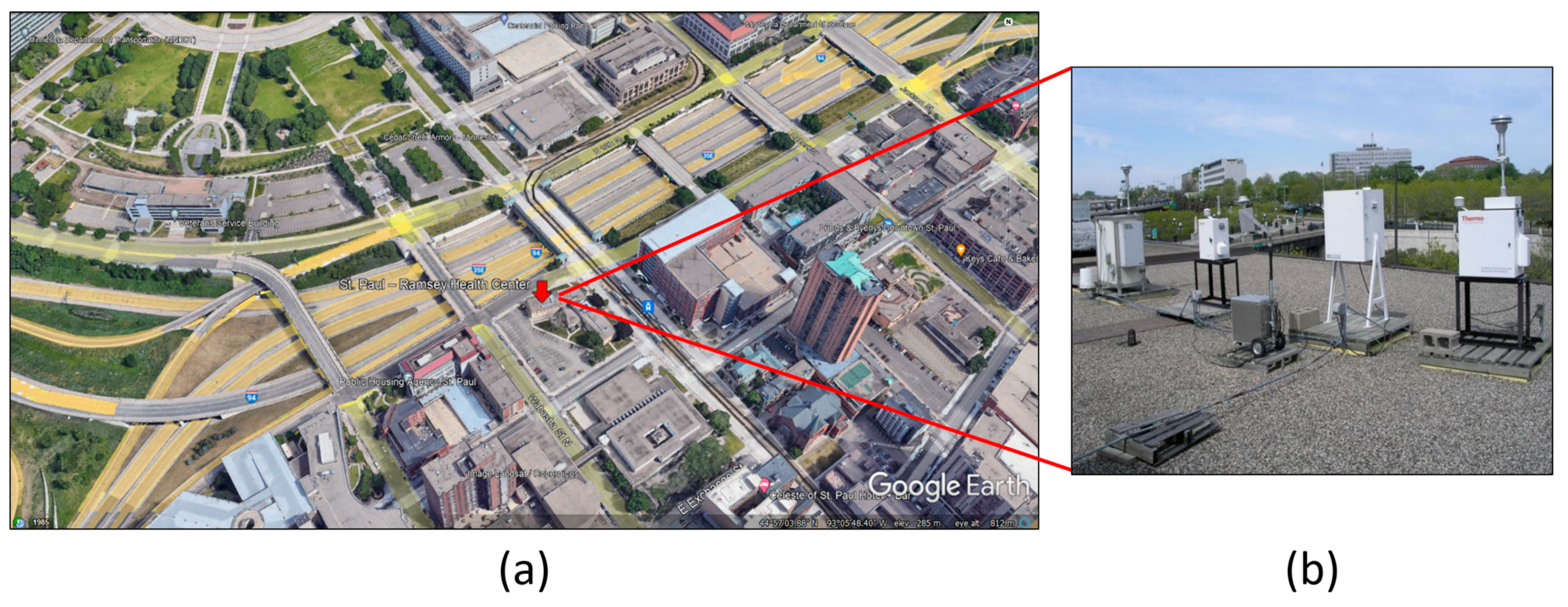
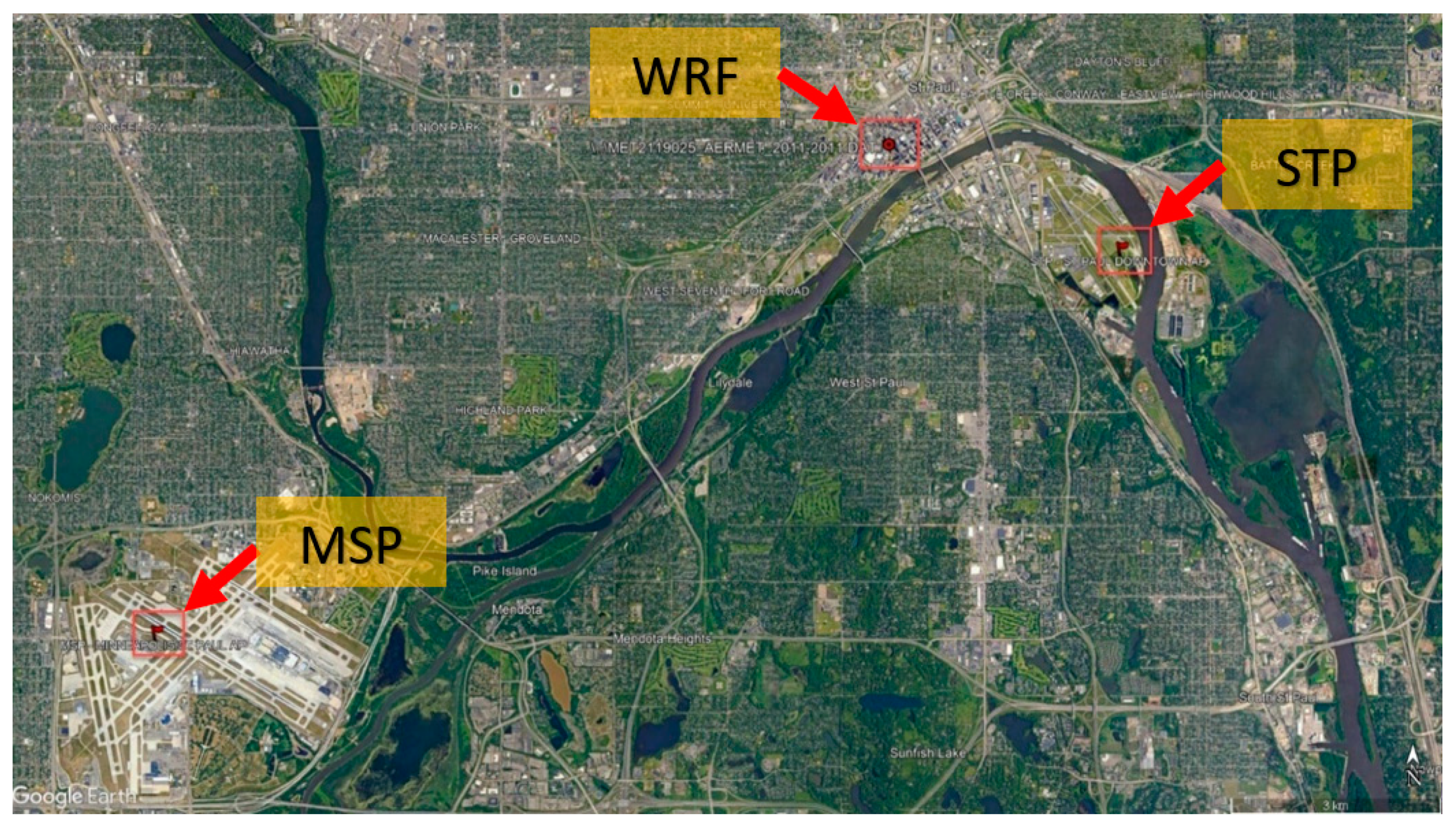
The near-road air monitoring site used to validate the air dispersion model is the Saint Paul—Ramsey Health Center. The Saint Paul—Ramsey Health Center monitoring site is located at 44°57′2.50″ N, 93° 5′54.60″ W and was chosen to be the project center. The station base elevation is 251 m above sea level, and the monitors are positioned on the north side of the building, approximately 60 m south of the Interstate-94 corridor and interchange with Interstate-35E. The station measures the following pollutants: PM₁₀, PM_2.5, metals, CO, carbonyls, O₃, SO₂, NO_x, asbestos, and volatile organic compounds (VOCs) [75].

This monitoring site was chosen to validate the air dispersion model because of the

• Proximity to the modeled high-traffic roadway segments;
• Absence of other sources within the project area. This increases the confidence of attributing the concentrations to the high-traffic roadway segments;
• Availability of model to monitor ratio data for MSATs.

Figure 13a shows the location of the Saint Paul—Ramsey Health Center monitoring site. The monitoring equipment is displayed in Figure 13b.

The MSATs included in the validation study are benzene and formaldehyde. After completing the air dispersion modeling, the modeled results were compared with the monitored concentrations at the near-road monitoring site. Comparing modeled and monitored concentrations is critical in evaluating how the air dispersion model performs. Using data from air monitoring stations to validate the air dispersion model performance is known as the validation of the model or model calibration. Calibrating the model is an iterative process used to improve the model performance and lower the uncertainty associated with the data.

Table 16. Modeled On-Road Air Concentrations Compared to Annual Mean Monitored Concentrations at the Saint Paul—Ramsey Health Center Monitoring Site.

Benzene—Annual Values
Modeled (On-road)	1.11	µg/m3
MPCA Monitored	0.71	µg/m3
MPCA Modeled	1.90	µg/m3
On-road Modeled Source Contribution	72%	-
MPCA Modeled (On-road)	1.37	µg/m3
MPCA Monitored—Assuming On-road Contribution is 72.0%	0.51	µg/m3
MPCA Modeled/MPCA Monitored (Ratio)	2.68	-
Modeled (On-road)/MPCA Monitored (Ratio)	2.17	-
Formaldehyde—Annual Values
Modeled (On-road)	1.10	µg/m3
MPCA Monitored	2.20	µg/m3
MPCA Modeled	2.60	µg/m3
On-road Modeled Source Contribution	36%	-
MPCA Modeled (On-road)	0.94	µg/m3
MPCA Monitored—Assuming On-road Contribution is 36.0%	0.79	µg/m3
MPCA Modeled/MPCA Monitored (Ratio)	1.18	-
Modeled (On-road)/MPCA Monitored (Ratio)	1.39	-

summarizes the modeled on-road air concentrations compared to annual mean monitored concentrations at the Saint Paul—Ramsey Health Center monitoring site.

The ratios presented in Table 16 conform with the often-quoted factor of two accuracy, a ratio recognized in the air dispersion modeling field. The validation of the air dispersion model demonstrated reasonable agreement between the modeled concentrations and the available measurements at the near-road air monitoring site, even though results varied among benzene and formaldehyde, and the modeled concentrations were higher than the measurements. The MPCA monitored concentrations and source contribution percentages were obtained from MPCAs’ MNRISKS Model-Monitor Tool [76].

4.3. Air Dispersion Model Performance

In the Validation of Methodology subsection, it was determined that the air dispersion model’s performance is deemed acceptable because the annual modeled concentrations of benzene and formaldehyde are within a factor of two [77] of the corresponding observed concentrations. Additionally, two statistical indicators were calculated to assess the model’s performance: fractional bias (FB) and normalized mean square error (NMSE) [78]. FB and NMSE were calculated using the equations shown below, and the values of these statistical indicators are summarized in

Table 17. Air Dispersion Model Performance Statistics.

Statistical Indicator	Formaldehyde	Benzene
Fractional Bias	−0.33	−0.74
Normalized Mean Square Error	0.11	0.64

.

$$\mathrm{FB}=2\left(\frac{\overline{C_0}-\overline{C_p}}{\overline{C_0}+\overline{C_p}}\right)$$

(5)

$$\mathrm{NMSE}=\frac{\overline{{\left(C_0-C_p\right)}^2}}{\overline{C_0}\overline{C_p}}$$

(6)

where C₀ represents the observed concentration, and C_p represents the modeled concentration.

An ideal air dispersion model would have both fractional bias and normalized mean square error equal to zero [78]. The fractional bias was selected as a performance measure because it is symmetrical and bounded, as referenced in [79]. A negative value of fractional bias indicates model overprediction.

4.4. Strengths and Limitations of the Methodology

In this subsection, we will discuss the strengths and limitations of the research methodology used in this study. Key strengths of the presented methodology are as follows:

• Integration of the results from three different types of models (i.e., on-road vehicle emissions inventory, air dispersion models, and risk estimate models), enabling the estimation of cumulative human health impacts from multiple exposure routes including direct inhalation and indirect ingestion of MSATs. Heath impact assessments include chronic cancer (i.e., risk) and noncancer health effects (i.e., hazard) as well as shortly term acute exposure to MSATs.
• Incorporation of spatiotemporal considerations to improve the characterization of emissions and resulting health impacts to represent real-world exposures more realistically.

It is worth noting that the methodology being presented has certain limitations, which are summarized below:

• It uses average values for key exposure parameters, such as body weight and inhalation rate, which may not accurately reflect the variability in the population. To address this limitation, follow-up research is being conducted to develop a new stochastic risk characterization model (discussed in the Conclusions section), enabling the assessment of risks across a range of population groups (e.g., body weight by age groups), including those most susceptible to the effects of MSATs exposure. This will enable more targeted resource allocation and abatement measures for improved public health outcomes.
• The current exposure assessment does not consider exposure to non-mobile-source air toxics, such as indoor emissions from sources like wood-burning stoves, or air toxics formed by secondary reactions, such as the secondary formation of formaldehyde and acetaldehyde. While this type of exposure assessment is not currently planned, it would be valuable for future work.

4.5. Determining the Existence of Exposure Scenarios in the Study Area

Human health impacts from MSATs exposure are calculated and analyzed for multiple developed scenarios in this paper. The analyzed scenarios include Farmer Adult, Farmer Child, Urban Resident Adult, and Urban Resident Child. In this subsection, the likelihood of a developed scenario being realistic is discussed.

As revealed in the Risk Results, the farmer scenario drives the total individual cancer risk in the case of benzo(a)pyrene and the cumulative cancer risk at the Saint Paul—Ramsey Health Center and the Anderson Office Building sensitive receptors. However, both sensitive receptors (e.g., Saint Paul—Ramsey Health Center and Anderson Office Building) are in highly developed commercially zoned urban areas, meaning the likelihood of the farmer exposure scenario driving the risk at these locations is very low.

In addition, the exposure pathways for a farmer scenario are not likely to occur because the following exposure pathways are improbable in a highly developed urban area:

• Incidental ingestion (e.g., from hand-to-mouth contact) of soil.
• Ingestion of homegrown produce such as lettuce, potatoes, onion, or tomatoes.
• Ingestion of homegrown beef, chicken, eggs, or home-reared pork.

It is important in the human health risk assessment process to take a common-sense approach in analyzing the developed scenarios within a project domain and describing the probability of that scenario occurring or not, because if the exposure scenario does not occur in the study area, the relevant exposure pathways that represent the exposure scenario do not exist, and therefore no risk occurs. In this paper, the farmer scenario was included to demonstrate the different scenarios that can be applied and analyzed within the proposed methodology. Furthermore, the farmer scenario can be easily applied in other exposure settings, such as evaluating human health risks in a project area situated in agricultural land with major heavy diesel commercial motor vehicle operations, such as the Interstate 5 and California 99 intersection in the San Joaquin Valley, the United States’ most productive farming area.

4.6. Variability and Uncertainty Discussion

Several exposure parameters used in the risk and hazard characterization were represented by average values corresponding to the 50th percentile of the exposure factor distribution, such as body weight and metabolic rates. These values misrepresent the natural variability in a population and, therefore, will introduce uncertainty in the risk characterization and influence the results. Three dominant exposure parameters, along with their associated uncertainties, are described in this subsection. These parameters are body weight, inhalation rate, and consumption rate of animal tissue. These parameters are used in quantitatively estimating cancer risk and noncancer hazards.

4.6.1. Body Weight

The body weight (BW) parameter is used to calculate the MSATs intake via the ingestion exposure pathway [26], and the ratio of the consumption rate to the body weight is termed the dose.

The U.S. EPA’s recommended default BW values in deterministic human health risk assessments are 70 and 15 kg for adults and children, respectively [26], and these values were used in the case study presented in this paper. The values for this parameter are project-specific and might be higher or lower depending on the project location and the assessed population. Therefore, the default BW values might not accurately reflect the population’s actual body weights due to the intra-population variability. However, the degree of variation of the BW is not expected to impact the risk results significantly because, in the case of adults, the default value is within 25% of the true value for most adults [80].

4.6.2. Inhalation Rate

The inhalation rate parameter is used to estimate the average daily MSATs intake via the inhalation exposure pathway. The U.S. EPA’s recommended default values are 0.83 m³/h for adults and 0.3 m³/h for children [26]. The uncertainties associated with this parameter include varying inhalation rates amongst the population due to many factors, such as age, activity level, genes, and lifestyle. For example, a farmer or fisher exposure scenario may have an increased respiratory rate due to the strenuous activities involved in their jobs, such as heavy carrying and lifting. Moreover, farmers may have prolonged exposures to MSATs due to the proximity of their homes to their workplaces (e.g., farms).

4.6.3. Consumption Rate of Animal Tissue

The consumption rate of animal tissue is a critical parameter in estimating the daily intake of MSATs from the ingestion of animal tissue. This parameter represents the ingestion of pork, beef, milk, poultry, or eggs. The unit for this parameter is expressed in kg/kg-day on a fresh weight (FW) basis. The recommended default consumption rate values [26] used in this study are summarized in

Table 18. Recommended Default Animal Tissue Consumption Rate Values.

Animal Tissue (Homegrown)	kg/kg-day FW
	Farmer
	Adult	Child
Beef	0.00122	0.00075
Milk	0.01367	0.02268
Poultry	0.00066	0.00045
Eggs	0.00075	0.00054
Pork	0.00055	0.00042

.

The uncertainties associated with this parameter include employing default average values that are not representative of project-specific conditions. Moreover, these default values do not consider the relatively sizeable inter-person variability in dietary intake [81]. The variability associated with this parameter may underestimate or overestimate the studied population’s consumption rate of animal tissue and thus impact the exposure calculations.

As described in this subsection, significant sources of uncertainty in human health risk assessment include using default average values for dominant exposure parameters to represent the population without considering the natural variability in a studied population. As a result, default average values provide inadequate information about variability surrounding the risk from exposure.

Variability can be addressed using a stochastic model to improve the analysis by reducing the variability of data uncertainty. Moreover, reducing and characterizing the variability in a population can assist in focusing the analysis on segments of the population that may be at higher risk from environmental exposure. Future research is needed to address the variability issues by developing a new stochastic analysis-based risk characterization to describe better the risk posed to human health and the surrounding ecosystem.

5. Conclusions

This paper presents a novel and validated methodology to quantify the numerous potential health risks associated with exposure to Mobile Source Air Toxics emitted from on-road sources for the first time.

This methodology overcomes many existing gaps and limitations in the literature and current practices, such as roadway geometry characterization between different models, employing average emissions to calculate human health impacts, and assessing human health impacts from inhalation routes of exposure only. Not evaluating non-inhalation exposures does not reveal the full extent of health impacts from exposure to MSATs, especially with air toxics like benzo(a)pyrene, which builds up in the tissues of organisms.

This methodology integrates several academic disciplines, including the estimation of mobile source emissions of thousands of air toxics, the atmospheric dispersion and deposition of these toxics, the fate and transport of toxics through various media, the assessment of the dose on humans, and the computation of the cumulative cancer risks and noncancer hazards.

The methodology supports the identification of human health risk impacts from exposure to mobile source air toxics by using validated models to determine if the predicated direct (e.g., inhalation) and indirect (e.g., ingestion) risks in existing or proposed transportation projects exceed target risk levels. Moreover, the result of this work provides regulators and stakeholders with the information to evaluate the magnitude of potential human health risks.

Three MSATs were evaluated in this paper, and their modeled air concentrations were validated against monitored data. The validation of the air concentrations demonstrated reasonable agreement between the modeled concentrations and the available measurements at the Saint Paul—Ramsey Health Center monitoring site.

Risk results using the hybrid risk modeling approach show that exposure to benzo(a)pyrene has the potential to cause adverse human health effects based on the evaluation of the Farmer Adult scenario at the Saint Paul—Ramsey Health Center and Anderson Office Building sensitive receptor locations. As shown in Table 12, for the farmer scenario, the calculated total benzo(a)pyrene cancer risk is equal to 4.95E-05 at the Saint Paul—Ramsey Health Center and 2.02E-05 at the Anderson Office Building. While the Farmer Adult scenario was not applicable in this study area, other transportation corridors with traffic flows of the same magnitude exist where the Farmer Adult scenario would apply (e.g., Interstate 5 and California 99 intersection in the San Joaquin Valley). This conclusion is based on the fact that the estimated cancer risks using modeled air toxics concentrations at the referenced sensitive receptors are above the target risk levels published in Table 5. Synthesizing the results from the air dispersion and deposition model and the hybrid risk model leads to inferences that:

• On-road mobile sources have the potential pose serious health concerns due to the proximity of these emission sources to human receptors;
• Human receptors are exposed to MSATs via direct pathways such as inhalation and indirect pathways, where the MSATs pass through another environmental medium, such as the ingestion of contaminated food. Risks from indirect pathways further contribute to risk already attributed to the inhalation exposure pathway. Risks from non-inhalation pathways are likely higher than inhalation risks.

Evaluating human health risk using default average estimates for important dominant exposure variables such as body weight or inhalation rates does not provide sufficient information about the variability surrounding the human health risk from exposure. Additional research is recommended to address the variability in the population by developing a new stochastic analysis-based risk characterization to better describe the risk posed to human health and the surrounding ecosystem. Moreover, it is recommended to implement the first deterministic ecological health assessment methodology for Mobile Source Air Toxics to understand the magnitude of damage done to the ecosystem as a result of air toxics exposure. Lastly, this research lends itself to incorporating risk driver analyses to aid in detecting and uncovering exposure scenarios with adverse impacts that are not well-known or well-studied, such as exploring the risks from endocrine disruptors or the consequences of DNA methylation.

References

1. Kuehn, B.M. WHO: More than 7 Million Air Pollution Deaths Each Year. JAMA 2014, 311, 1486. [Google Scholar] [CrossRef] [PubMed]
2. World Health Organization. Ambient Air Pollution: A Global Assessment of Exposure and Burden of Disease; World Health Organization: Geneva, Switzerland, 2016. [Google Scholar]
3. American Lung Association. State of the Air 2019; American Lung Association: Chicago, IL, USA, 2019. [Google Scholar]
4. Landrigan, P.J.; Fuller, R.; Acosta, N.J.R.; Adeyi, O.; Arnold, R.; Basu, N.; Baldé, A.B.; Bertollini, R.; Bose-O’Reilly, S.; Boufford, J.I.; et al. The Lancet Commission on Pollution and Health. Lancet 2018, 391, 462–512. [Google Scholar] [CrossRef] [PubMed] [Green Version]
5. World Bank Group. The Cost of Air Pollution: Strengthening the Economic Case for Action; World Bank Group: Washington, DC, USA, 2016. (In English) [Google Scholar]
6. Health Effects Institute. Mobile-Source Air Toxics: A Critical Review of the Literature on Exposure and Health Effects; Health Effects Institute: Boston, NA, USA, 2007. [Google Scholar]
7. U.S. Environmental Protection Agency. The Master List of Compounds Emitted by Mobile Sources—2006; U.S. Environmental Protection Agency: Washington, DC, USA, 2006. [Google Scholar]
8. Hata, H.; Yamada, H.; Kokuryo, K.; Okada, M.; Funakubo, C.; Tonokura, K. Estimation Model for Evaporative Emissions from Gasoline Vehicles Based on Thermodynamics. Sci. Total Environ. 2018, 618, 1685–1691. [Google Scholar] [CrossRef] [PubMed]
9. Kam, W.; Liacos, J.W.; Schauer, J.J.; Delfino, R.J.; Sioutas, C. On-Road Emission Factors of PM Pollutants for Light-Duty Vehicles (LDVs) Based on Urban Street Driving Conditions. Atmos. Environ. 2012, 61, 378–386. [Google Scholar] [CrossRef]
10. Manisalidis, I.; Stavropoulou, E.; Stavropoulos, A.; Bezirtzoglou, E. Environmental and Health Impacts of Air Pollution: A Review. Front. Public Health 2020, 8, 14. [Google Scholar] [CrossRef] [Green Version]
11. Pratt, G.; Vadali, M.; Kvale, D.; Ellickson, K. Traffic, Air Pollution, Minority and Socio-Economic Status: Addressing Inequities in Exposure and Risk. Int. J. Environ. Res. Public Health 2015, 12, 5355–5372. [Google Scholar] [CrossRef] [Green Version]
12. Stoakes, J. Lakeshore Air Toxics Study Report; Indiana Department of Environmental Management: Indianapolis, IN, USA, 2013. [Google Scholar]
13. Pratt, G.C.; Dymond, M.; Ellickson, K.; Thé, J. Validation of a Novel Air Toxic Risk Model with Air Monitoring. Risk Anal. 2011, 32, 96–112. [Google Scholar] [CrossRef]
14. U.S. Environmental Protection Agency. Advice to EPA on Advancing the Science and Application of Ecological Risk Assessment in Environmental Decision-Making: A Report of the U.S. EPA Science Advisory Board; U.S. Environmental Protection Agency: Washington, DC, USA, 2007. [Google Scholar]
15. Apelberg, B.J.; Buckley, T.J.; White, R.H. Socioeconomic and Racial Disparities in Cancer Risk from Air Toxics in Maryland. Environ. Health Perspect. 2005, 113, 693–699. [Google Scholar] [CrossRef]
16. U.S. Environmental Protection Agency. 2014 NATA: Assessment Results. Available online: https://www.epa.gov/national-air-toxics-assessment/2014-nata-assessment-results (accessed on 2 April 2022).
17. Kaufman, J.D.; Elkind, M.S.V.; Bhatnagar, A.; Koehler, K.; Balmes, J.R.; Sidney, S.; Peña, M.S.B.; Dockery, D.W.; Hou, L.; Brook, R.D.; et al. Guidance to Reduce the Cardiovascular Burden of Ambient Air Pollutants: A Policy Statement from the American Heart Association. Circulation 2020, 142, e432–e447. [Google Scholar] [CrossRef]
18. Kingsley, S.L.; Eliot, M.N.; Carlson, L.; Finn, J.; MacIntosh, D.L.; Suh, H.H.; Wellenius, G.A. Proximity of US Schools to Major Roadways: A Nationwide Assessment. J. Expo. Sci. Environ. Epidemiol. 2014, 24, 253–259. [Google Scholar] [CrossRef] [Green Version]
19. Karner, A.A.; Eisinger, D.S.; Niemeier, D.A. Near-Roadway Air Quality: Synthesizing the Findings from Real-World Data. Environ. Sci. Technol. 2010, 44, 5334–5344. [Google Scholar] [CrossRef] [PubMed]
20. Brugge, D.; Durant, J.L.; Rioux, C. Near-Highway Pollutants in Motor Vehicle Exhaust: A Review of Epidemiologic Evidence of Cardiac and Pulmonary Health Risks. Environ. Health 2007, 6, 23. [Google Scholar] [CrossRef] [PubMed] [Green Version]
21. U.S. Environmental Protection Agency. PM Hot-Spot Guidance: Transportation Conformity Guidance for Quantitative Hot-Spot Analyses in PM2.5 and PM10 Nonattainment and Maintenance Areas; U.S. Environmental Protection Agency: Washington, DC, USA, 2021. [Google Scholar]
22. Healthy Environments and Consumer Safety Branch. Guidance for Evaluating Human Health Impacts in Environmental Assessment: Air Quality; Health Canada: Ottawa, ON, Canada, 2016. [Google Scholar]
23. U.S. Environmental Protection Agency. 1990 Clean Air Act Amendment Summary. Available online: https://www.epa.gov/clean-air-act-overview/1990-clean-air-act-amendment-summary (accessed on 11 February 2022).
24. Strum, M.; Scheffe, R. National Review of Ambient Air Toxics Observations. J. Air Waste Manag. Assoc. 2015, 66, 120–133. [Google Scholar] [CrossRef] [PubMed]
25. Galarneau, E.; Wang, D.; Dabek-Zlotorzynska, E.; Siu, M.; Celo, V.; Tardif, M.; Harnish, D.; Jiang, Y. Air Toxics in Canada Measured by the National Air Pollution Surveillance (NAPS) Program and Their Relation to Ambient Air Quality Guidelines. J. Air Waste Manag. Assoc. 2015, 66, 184–200. [Google Scholar] [CrossRef] [Green Version]
26. U.S. Environmental Protection Agency. Human Health Risk Assessment Protocol (HHRAP) for Hazardous Waste Combustion Facilities, Final; U.S. Environmental Protection Agency: Washington, DC, USA, 2005. [Google Scholar]
27. McKone, T.E. Assessing Multiple Pathway Exposures: Variability, Uncertainty, and Ignorance. In Municipal Waste Incineration Risk Assessment; Travis, C., Ed.; Springer: Boston, MA, USA, 1991; Volume 5, pp. 217–239. [Google Scholar] [CrossRef]
28. Dopico, M.; Gómez, A. Review of the Current State and Main Sources of Dioxins around the World. J. Air Waste Manag. Assoc. 2015, 65, 1033–1049. [Google Scholar] [CrossRef]
29. Smit, R.; Zeise, K.; Caffin, A.; Anyon, P. Dioxins Emissions from Motor Vehicles in Australia, National Dioxins Program Technical Report No. 2; Department of the Environment and Heritage: Canberra, Australia, 2004. [Google Scholar]
30. Geueke, K.-J.; Gessner, A.; Quass, U.; Bröker, G.; Hiester, E. PCDD/F Emissions from Heavy Duty Vehicle Diesel Engines. Chemosphere 1999, 38, 2791–2806. [Google Scholar] [CrossRef]
31. Gertler, A.W.; Sagebiel, J.C.; Dippel, W.A.; Farina, R.J. Measurements of Dioxin and Furan Emission Factors from Heavy-Duty Diesel Vehicles. J. Air Waste Manag. Assoc. 1998, 48, 276–278. [Google Scholar] [CrossRef] [Green Version]
32. Kanan, S.; Samara, F. Dioxins and Furans: A Review from Chemical and Environmental Perspectives. Trends Environ. Anal. Chem. 2018, 17, 1–13. [Google Scholar] [CrossRef]
33. Hanano, A.; Almousally, I.; Shaban, M.; Moursel, N.; Shahadeh, A.; Alhajji, E. Differential Tissue Accumulation of 2,3,7,8-Tetrachlorinated Dibenzo-p-Dioxin in Arabidopsis Thaliana Affects Plant Chronology, Lipid Metabolism and Seed Yield. BMC Plant Biol. 2015, 15, 193. [Google Scholar] [CrossRef] [Green Version]
34. U.S. Environmental Protection Agency. Integrated Modeling for Integrated Environmental Decision Making; U.S. Environmental Protection Agency: Washington, DC, USA, 2008. [Google Scholar]
35. Office of Air Quality Planning and Standards. Air Toxics Risk Assessment Reference Library: Volume 3—Community-Scale Assessment; U.S. Environmental Protection Agency: Durham, NC, USA, 2006. [Google Scholar]
36. Minnesota Pollution Control Agency. MNRISKS, Minnesota Statewide Screening of Human Health Risks from Air Pollution; Minnesota Pollution Control Agency: Saint Paul, MN, USA, 2022. [Google Scholar]
37. Conklin, D.J.; Malovichko, M.V.; Zeller, I.; Das, T.P.; Krivokhizhina, T.V.; Lynch, B.H.; Lorkiewicz, P.; Agarwal, A.; Wickramasinghe, N.; Haberzettl, P.; et al. Biomarkers of Chronic Acrolein Inhalation Exposure in Mice: Implications for Tobacco Product-Induced Toxicity. Toxicol. Sci. 2017, 158, 263–274. [Google Scholar] [CrossRef] [Green Version]
38. Ellickson, K.M.; Sevcik, S.M.; Burman, S.; Pak, S.; Kohlasch, F.; Pratt, G.C. Cumulative Risk Assessment and Environmental Equity in Air Permitting: Interpretation, Methods, Community Participation and Implementation of a Unique Statute. Int. J. Environ. Res. Public Health 2011, 8, 4140–4159. [Google Scholar] [CrossRef] [PubMed] [Green Version]
39. Agency for Toxic Substances and Disease Registry. Toxicological Profile for Benzene; U.S. Department of Health and Human Services: Washington, DC, USA, 2007. [Google Scholar]
40. World Health Organization. Benzene—IARC Monographs on the Evaluation of Carcinogenic Risks to Humans; World Health Organization: Lyon, France, 2018. [Google Scholar]
41. Pearson, R.L.; Wachtel, H.; Ebi, K.L. Distance-Weighted Traffic Density in Proximity to a Home Is a Risk Factor for Leukemia and Other Childhood Cancers. J. Air Waste Manag. Assoc. 2000, 50, 175–180. [Google Scholar] [CrossRef] [Green Version]
42. World Health Organization. Formaldehyde, 2-Butoxyethanol and 1-Tert-Butoxypropan-2-Ol—IARC Monographs on the Evaluation of Carcinogenic Risks to Humans; World Health Organization: Lyon, France, 2006. [Google Scholar]
43. National Toxicology Program. 15th Report on Carcinogens; U.S. Department of Health and Human Services: Durham, NC, USA, 2021. [Google Scholar]
44. World Health Organization. Benzo[A]Pyrene—IARC Monographs on the Evaluation of Carcinogenic Risks to Humans; World Health Organization: Lyon, France, 2010. [Google Scholar]
45. National Center for Environmental Assessment. Toxicological Review of Benzo[A]Pyrene; U.S. Environmental Protection Agency: Washington, DC, USA, 2017. [Google Scholar]
46. Whaley, C.H.; Galarneau, E.; Makar, P.A.; Moran, M.D.; Zhang, J. How Much Does Traffic Contribute to Benzene and Polycyclic Aromatic Hydrocarbon Air Pollution? Results from a High-Resolution North American Air Quality Model Centred on Toronto, Canada. Atmos. Chem. Phys. 2020, 20, 2911–2925. [Google Scholar] [CrossRef] [Green Version]
47. Schraufnagel, D.E. The Health Effects of Ultrafine Particles. Exp. Mol. Med. 2020, 52, 311–317. [Google Scholar] [CrossRef] [PubMed] [Green Version]
48. Office of Transportation and Air Quality. MOVES2014, MOVES2014a, and MOVES2014b Technical Guidance: Using MOVES to Prepare Emission Inventories for State Implementation Plans and Transportation Conformity; U.S. Environmental Protection Agency: Ann Arbor, MI, USA, 2018. [Google Scholar]
49. Jesse, L.T.; Cristiane, L.T.; Johnson, M.A.; Chamberlin, R.; National Cooperative Highway Research Program; Transportation Research Board; National Academies of Sciences, Engineering, and Medicine. Volume 1: TRAQS User Guide; Transportation Research Board: Washington, DC, USA, 2018. [Google Scholar]
50. U.S. Environmental Protection Agency. AERMOD Modeling System Development. Available online: https://www.epa.gov/scram/aermod-modeling-system-development (accessed on 1 August 2022).
51. AERMOD View, 19191 Lakes Environmental Software: Waterloo. 2019. Available online: https://www.weblakes.com/software/air-dispersion/aermod-view (accessed on 10 February 2022).
52. Skamarock, W.; Klemp, J.; Dudhia, J.; Gill, D.; Barker, D.; Duda, M.; Huang, X.; Wang, W.; Powers, J. A Description of the Advanced Research WRF Version 3; University Corporation for Atmospheric Research: Boulder, CO, USA, 2008. [Google Scholar]
53. Office of Air Quality Planning and Standards. Guidance on the Use of the Mesoscale Model Interface Program (MMIF) for AERMOD Applications; U.S. Environmental Protection Agency: Durham, NC, USA, 2022. [Google Scholar]
54. MacDonell, M.M.; Hertzberg, R.C.; Rice, G.E.; Wright, J.M.; Teuschler, L.K. Characterizing Risk for Cumulative Risk Assessments. Risk Anal. 2017, 38, 1183–1201. [Google Scholar] [CrossRef] [PubMed]
55. U.S. Environmental Protection Agency. Integrated Risk Information System. Available online: https://www.epa.gov/iris (accessed on 2 July 2022).
56. California Office of Environmental Health Hazard Assessment. Chemicals. Available online: https://oehha.ca.gov/chemicals (accessed on 21 October 2022).
57. Agency for Toxic Substances and Disease Registry. Toxic Substances Portal. Available online: https://wwwn.cdc.gov/TSP/index.aspx (accessed on 9 December 2022).
58. Region 6, U.S. EPA Multimedia Planning and Permitting Division. Region 6 Risk Management Addendum—Draft Human Health Risk Assessment Protocol for Hazardous Waste Combustion Facilities; U.S. Environmental Protection Agency: Dallas, TX, USA, 1998. [Google Scholar]
59. IRAP-h View, 5.1.1; Lakes Environmental Software: Waterloo. 2022. Available online: https://www.weblakes.com/software/risk-assessment/irap-h-view (accessed on 10 March 2022).
60. Minnesota Department of Transportation. Traffic Forecasting & Analysis. Available online: https://www.dot.state.mn.us/traffic/data/coll-methods.html (accessed on 2 January 2022).
61. Office of Air Quality Planning and Standards. Haul Road Workgroup Final Report; U.S. Environmental Protection Agency: Durham, NC, USA, 2012. [Google Scholar]
62. U.S. Environmental Protection Agency. Revisions to the Guideline on Air Quality Models: Enhancements to the AERMOD Dispersion Modeling System and Incorporation of Approaches to Address Ozone and Fine Particulate Matter; U.S. Environmental Protection Agency: Washington, DC, USA, 2017; Volume 40. [Google Scholar]
63. WRPLOT View, 8.0.2; Lakes Environmental Software: Waterloo. 2018. Available online: https://www.weblakes.com/software/freeware/wrplot-view (accessed on 5 March 2022).
64. Kemball-Cook, S.; Jia, Y.; Emery, C.; Morris, R. Alaska MM5 Modeling for the 2002 Annual Period to Support Visibility Modeling; UCR: Novato, CA, USA, 2005. [Google Scholar]
65. Bhati, S.; Mohan, M. WRF-Urban Canopy Model Evaluation for the Assessment of Heat Island and Thermal Comfort over an Urban Airshed in India under Varying Land Use/Land Cover Conditions. Geosci. Lett. 2018, 5, 27. [Google Scholar] [CrossRef] [Green Version]
66. Watson, A.Y.; Bates, R.R.; Kennedy, D. Air Pollution, the Automobile, and Public Health; National Academy Press: Washington, DC, USA, 1988. [Google Scholar]
67. Kim, K.H.; Lee, S.-B.; Woo, D.; Bae, G.-N. Influence of Wind Direction and Speed on the Transport of Particle-Bound PAHs in a Roadway Environment. Atmos. Pollut. Res. 2015, 6, 1024–1034. [Google Scholar] [CrossRef]
68. Wagner, P.; Schäfer, K. Influence of Mixing Layer Height on Air Pollutant Concentrations in an Urban Street Canyon. Urban Clim. 2017, 22, 64–79. [Google Scholar] [CrossRef]
69. Geiß, A.; Wiegner, M.; Bonn, B.; Schäfer, K.; Forkel, R.; von Schneidemesser, E.; Münkel, C.; Chan, K.L.; Nothard, R. Mixing Layer Height as an Indicator for Urban Air Quality? Atmos. Meas. Tech. 2017, 10, 2969–2988. [Google Scholar] [CrossRef] [Green Version]
70. Regional Office for Europe & Joint WHO/Convention Task Force on the Health Aspects of Air Pollution. Health Risks of Particulate Matter from Long-Range Transboundary Air Pollution; World Health Organization: Copenhagen, Denmark, 2006. [Google Scholar]
71. Schreiberová, M.; Vlasáková, L.; Vlček, O.; Šmejdířová, J.; Horálek, J.; Bieser, J. Benzo[A]Pyrene in the Ambient Air in the Czech Republic: Emission Sources, Current and Long-Term Monitoring Analysis and Human Exposure. Atmosphere 2020, 11, 955. [Google Scholar] [CrossRef]
72. National Library of Medicine. Benzo(a)pyrene, Hazardous Substances DataBank Number 2554. Available online: https://pubchem.ncbi.nlm.nih.gov/source/hsdb/2554 (accessed on 31 October 2022).
73. Lan, Q.; Zhang, L.; Li, G.; Vermeulen, R.; Weinberg, R.S.; Dosemeci, M.; Rappaport, S.M.; Shen, M.; Alter, B.P.; Wu, Y.; et al. Hematotoxicity in Workers Exposed to Low Levels of Benzene. Science 2004, 306, 1774–1776. [Google Scholar] [CrossRef] [PubMed] [Green Version]
74. National Center for Environmental Assessment. Formaldehyde; CASRN 50-00-0; U.S. Environmental Protection Agency: Washington, DC, USA, 1990. [Google Scholar]
75. Minnesota Pollution Control Agency. 2023 Air Monitoring Network Plan for Minnesota; Minnesota Pollution Control Agency: Saint Paul, MN, USA, 2022. [Google Scholar]
76. Kvale, D. MnRiskS Model-Monitor Tool. Available online: https://public.tableau.com/views/MnRiskSModel-MonitorTool1/Dashboard1?%3Aembed=y (accessed on 1 October 2022).
77. Valencia, A.; Venkatram, A.; Heist, D.; Carruthers, D.; Arunachalam, S. Development and Evaluation of the R-LINE Model Algorithms to Account for Chemical Transformation in the Near-Road Environment. Transp. Res. Part D Transp. Environ. 2018, 59, 464–477. [Google Scholar] [CrossRef] [PubMed] [Green Version]
78. Chang, J.C.; Hanna, S.R. Air Quality Model Performance Evaluation. Meteorol. Atmos. Phys. 2004, 87, 167–196. [Google Scholar] [CrossRef]
79. Cox, W.M.; Tikvart, J.A. A Statistical Procedure for Determining the Best Performing Air Quality Simulation Model. Atmos. Environment. Part A Gen. Top. 1990, 24, 2387–2395. [Google Scholar] [CrossRef]
80. National Research Council (U.S.). Committee On Risk Assessment of Hazardous Air Pollutants. Science and Judgment in Risk Assessment; National Academy Press: Washington, DC, USA, 1994. [Google Scholar]
81. Hebert, J.; Gupta, P.; Mehta, H.; Ebbeling, C.; Bhonsle, R.; Varghese, F. Sources of Variability in Dietary Intake in Two Distinct Regions of Rural India: Implications for Nutrition Study Design and Interpretation. Eur. J. Clin. Nutr. 2000, 54, 479–486. [Google Scholar] [CrossRef] [Green Version]
82. Willmott, C.; Matsuura, K. Advantages of the Mean Absolute Error (MAE) over the Root Mean Square Error (RMSE) in Assessing Average Model Performance. Clim. Res. 2005, 30, 79–82. [Google Scholar] [CrossRef]
Figure 1. Flowchart of the Proposed Methodology.
Atmosphere 14 00506 g001
Figure 2. Transportation Air Quality System (TRAQS) Graphical User Interface.
Atmosphere 14 00506 g002
Figure 3. Location of High-Traffic Road Segments on the Interstate-35E. Map Data: Google Maps.
Atmosphere 14 00506 g003
Figure 4. Wind Rose Plot Showing the Wind Patterns at the Project Center for CY 2011.
Atmosphere 14 00506 g004
Figure 5. Benzene Hourly Air Concentration—Vapor Phase (Unitized) Contour Plot overlaid on OpenStreetMap Satellite Imagery (OpenStreetMap, n.d.). Unit used in contour is µg-s/g-m3.
Atmosphere 14 00506 g005
Figure 6. Benzene Annual Air Concentration—Vapor Phase (Unitized) Contour Plot overlaid on OpenStreetMap Satellite Imagery (OpenStreetMap, n.d.). Unit used in contour is µg-s/g-m3.
Atmosphere 14 00506 g006
Figure 7. Formaldehyde Hourly Air Concentration—Vapor Phase (Unitized) Contour Plot overlaid on OpenStreetMap Satellite Imagery (OpenStreetMap, n.d.). Unit used in contour is µg-s/g-m3.
Atmosphere 14 00506 g007
Figure 8. Formaldehyde Annual Air Concentration—Vapor Phase (Unitized) Contour Plot overlaid on OpenStreetMap Satellite Imagery (OpenStreetMap, n.d.). Unit used in contour is µg-s/g-m3.
Atmosphere 14 00506 g008
Figure 9. BaP Hourly Air Concentration—Vapor Phase (Unitized) Contour Plot overlaid on OpenStreetMap Satellite Imagery (OpenStreetMap, n.d.). Unit used in contour is µg-s/g-m3.
Atmosphere 14 00506 g009
Figure 10. BaP Hourly Air Concentration—Particle-Bound Phase (Unitized) Contour Plot overlaid on OpenStreetMap Satellite Imagery (OpenStreetMap, n.d.). Unit used in contour is µg-s/g-m3.
Atmosphere 14 00506 g010
Figure 11. BaP Annual Air Concentration—Vapor Phase (Unitized) Contour Plot overlaid on OpenStreetMap Satellite Imagery (OpenStreetMap, n.d.). Unit used in contour is µg-s/g-m3.
Atmosphere 14 00506 g011
Figure 12. BaP Annual Air Concentration—Particle-Bound Phase (Unitized) Contour Plot overlaid on OpenStreetMap Satellite Imagery (OpenStreetMap, n.d.). Unit used in contour is µg-s/g-m3.
Atmosphere 14 00506 g012
Figure 13. (a) Saint Paul—Ramsey Health Center Monitoring Site. Map Data: Google Earth (b) Monitoring Equipment. Photo: Minnesota Pollution Control Agency.
Atmosphere 14 00506 g013