
Analyzing and Modeling the Spatial-Temporal Changes and the Impact of GLOTI Index on Precipitation in the Marmara Region of Türkiye

 , , , and
Abstract
:1. Introduction
- ○
- To study the general situation of precipitation in the Marmara region during the last 61 years.
- ○
- To analyze the changes and variations of precipitation trends in the Marmara region during the last 61 years.
- ○
- Investigation of the annual and seasonal spatial distribution of precipitation in the Marmara region.
- ○
- Analysis of the impact of climate change and global warming on precipitation in the Marmara region.
- ○
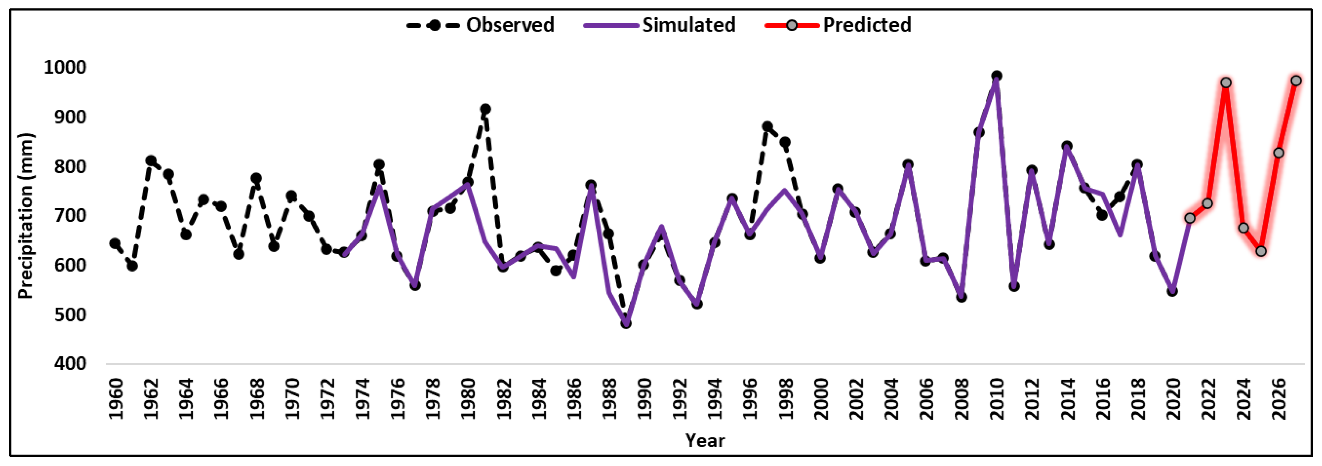
- Modeling and prediction of precipitation in the Marmara region for the next 7 years.
2. Data and Methods
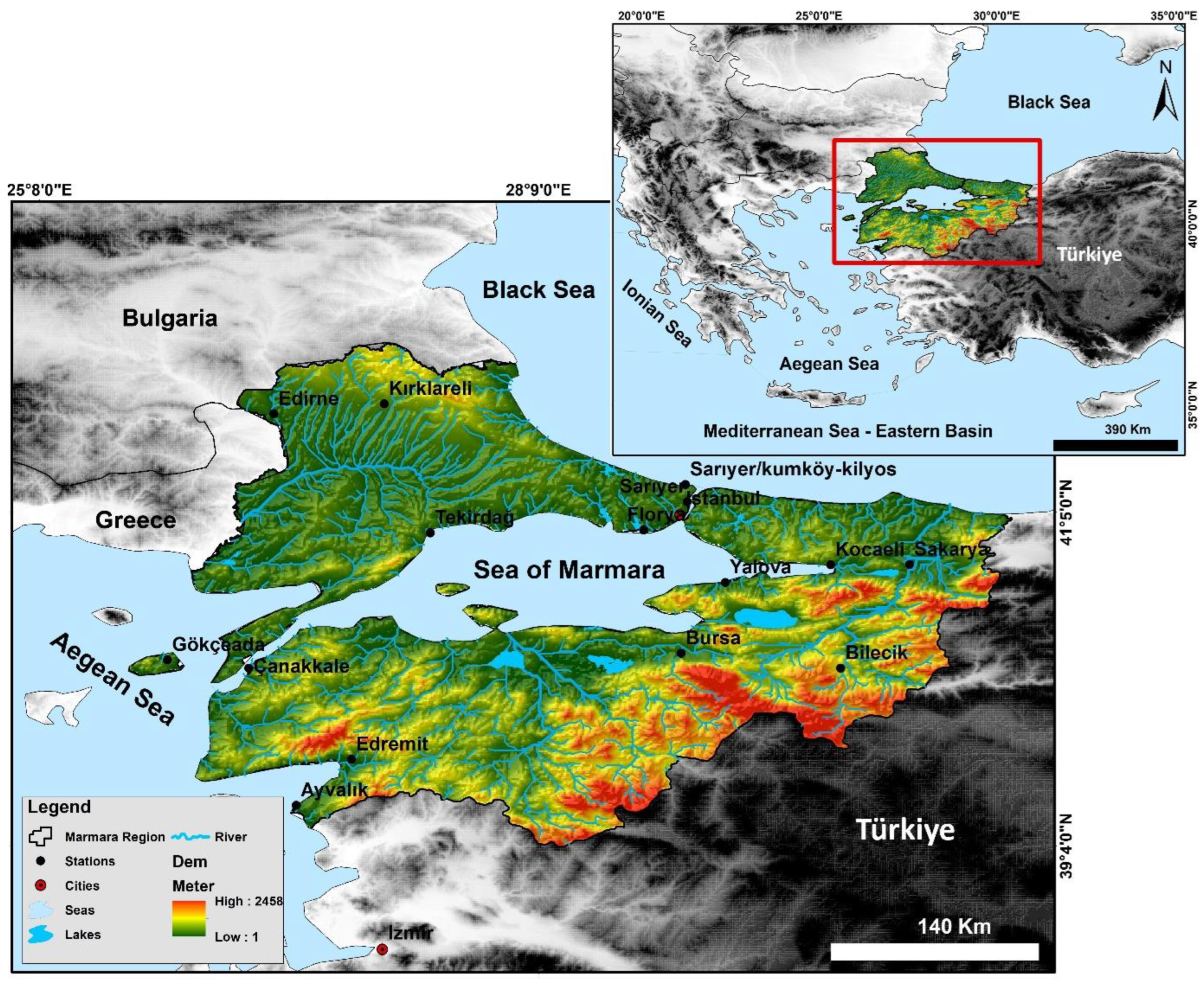
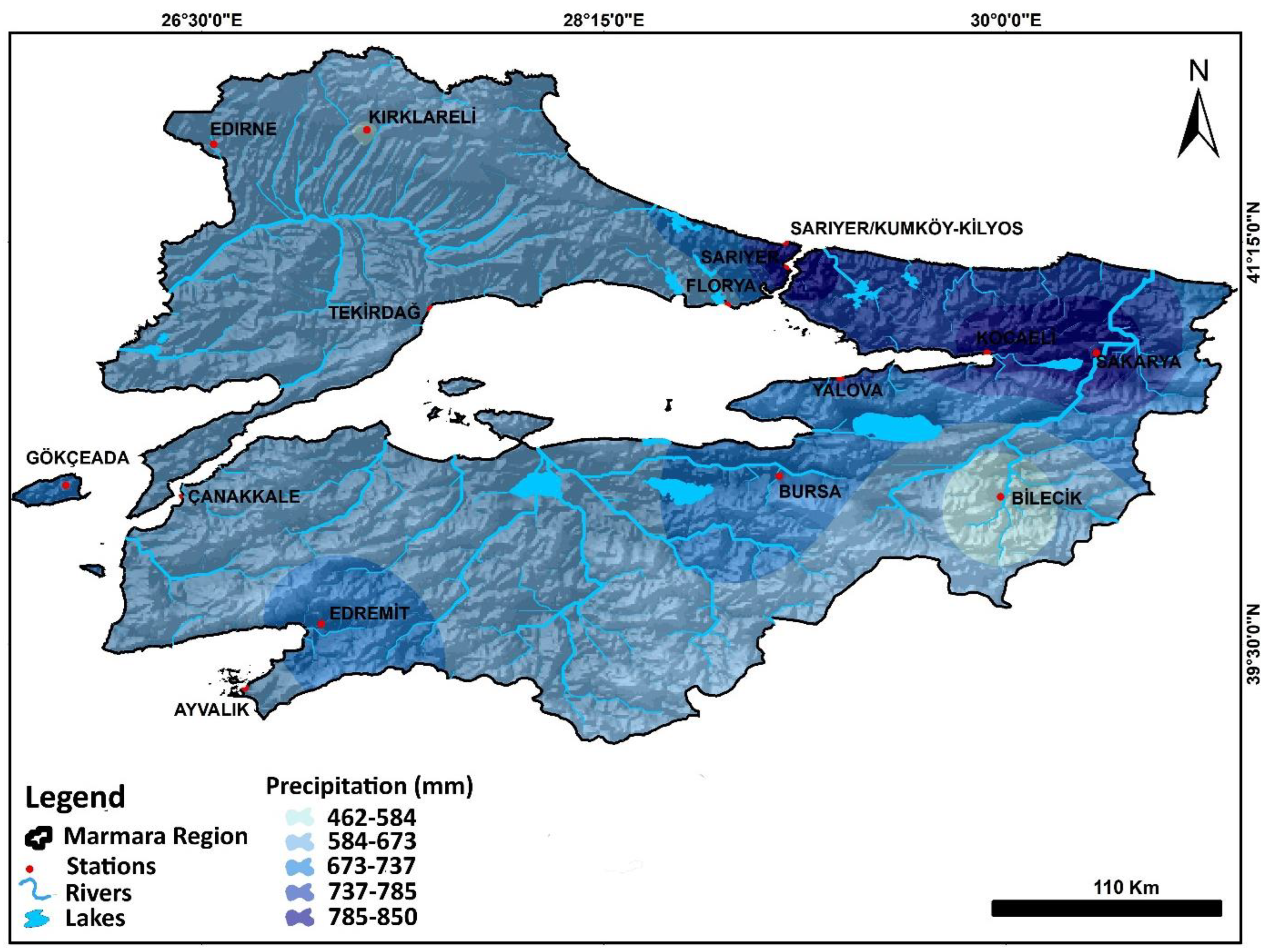
2.1. Study Area
2.2. Data
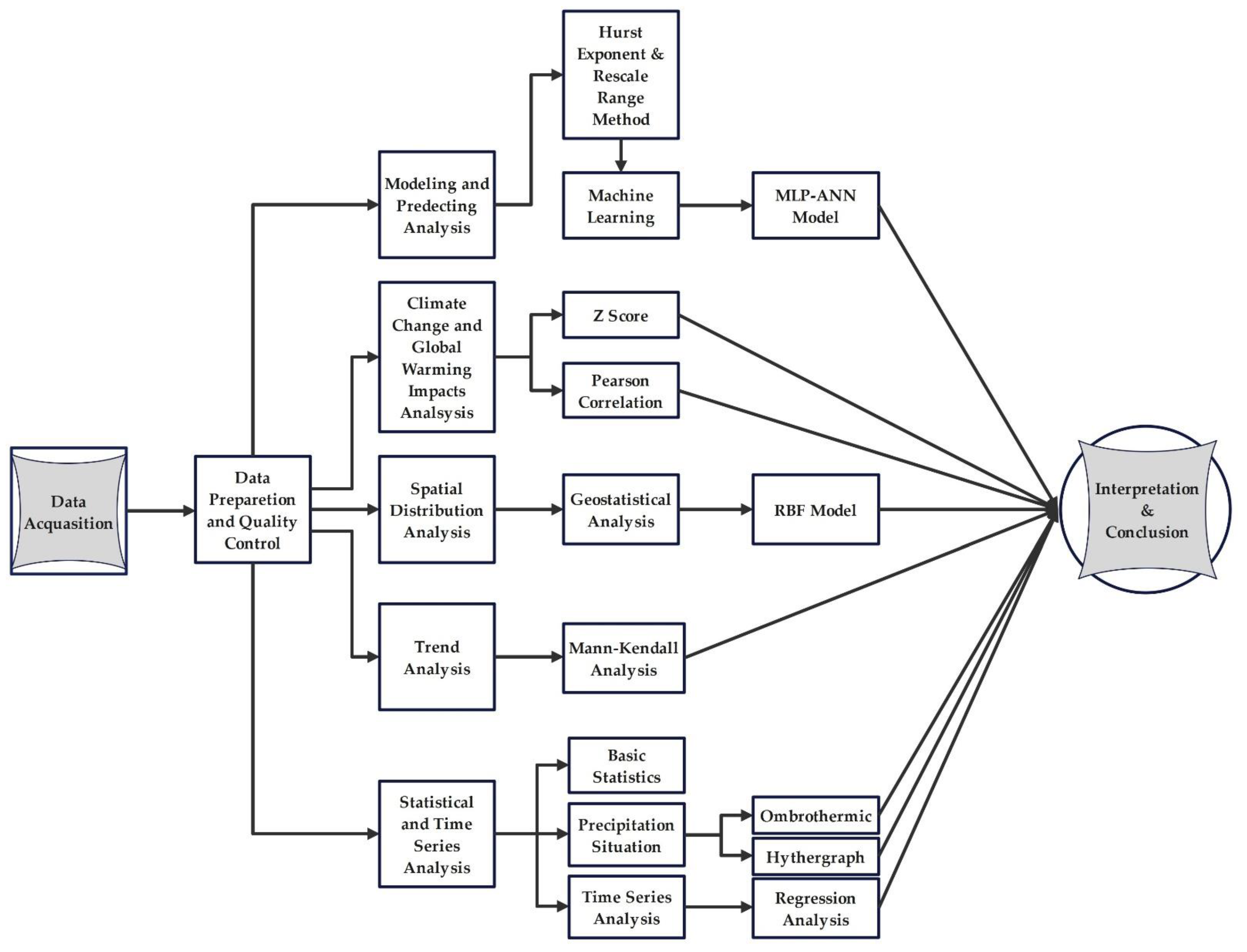
2.3. Methods
2.4. Nonparametric Testing
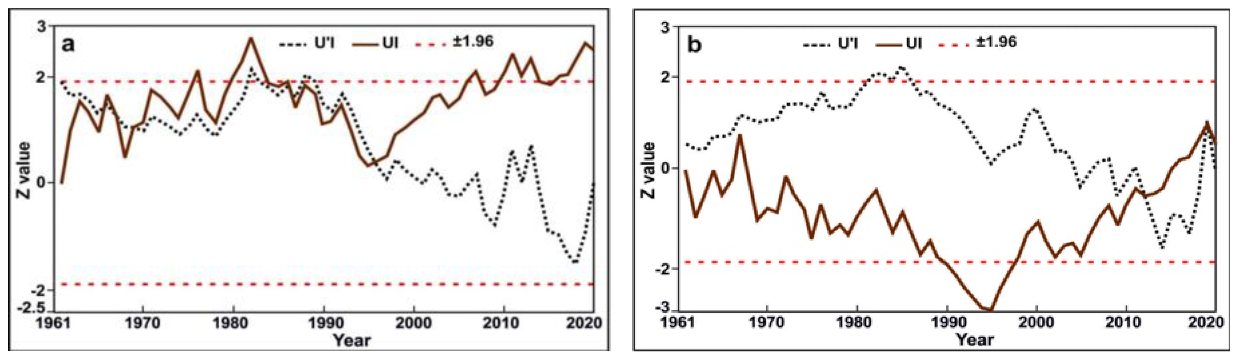
2.5. Mann-Kendall Test-Detection of Mutations
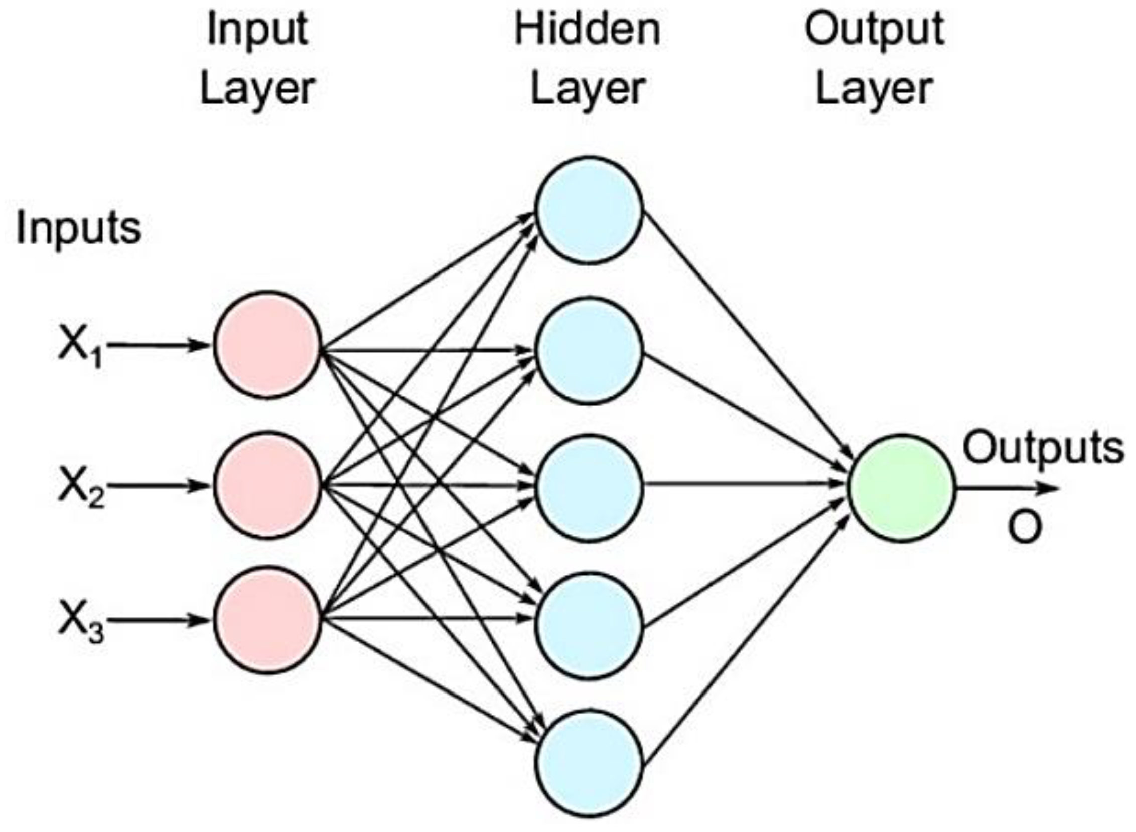
2.6. MLP-ANN Model

2.7. Broyden–Fletcher–Goldfarb–Shanno Algorithm (BFGS)
2.8. Normalization of Data
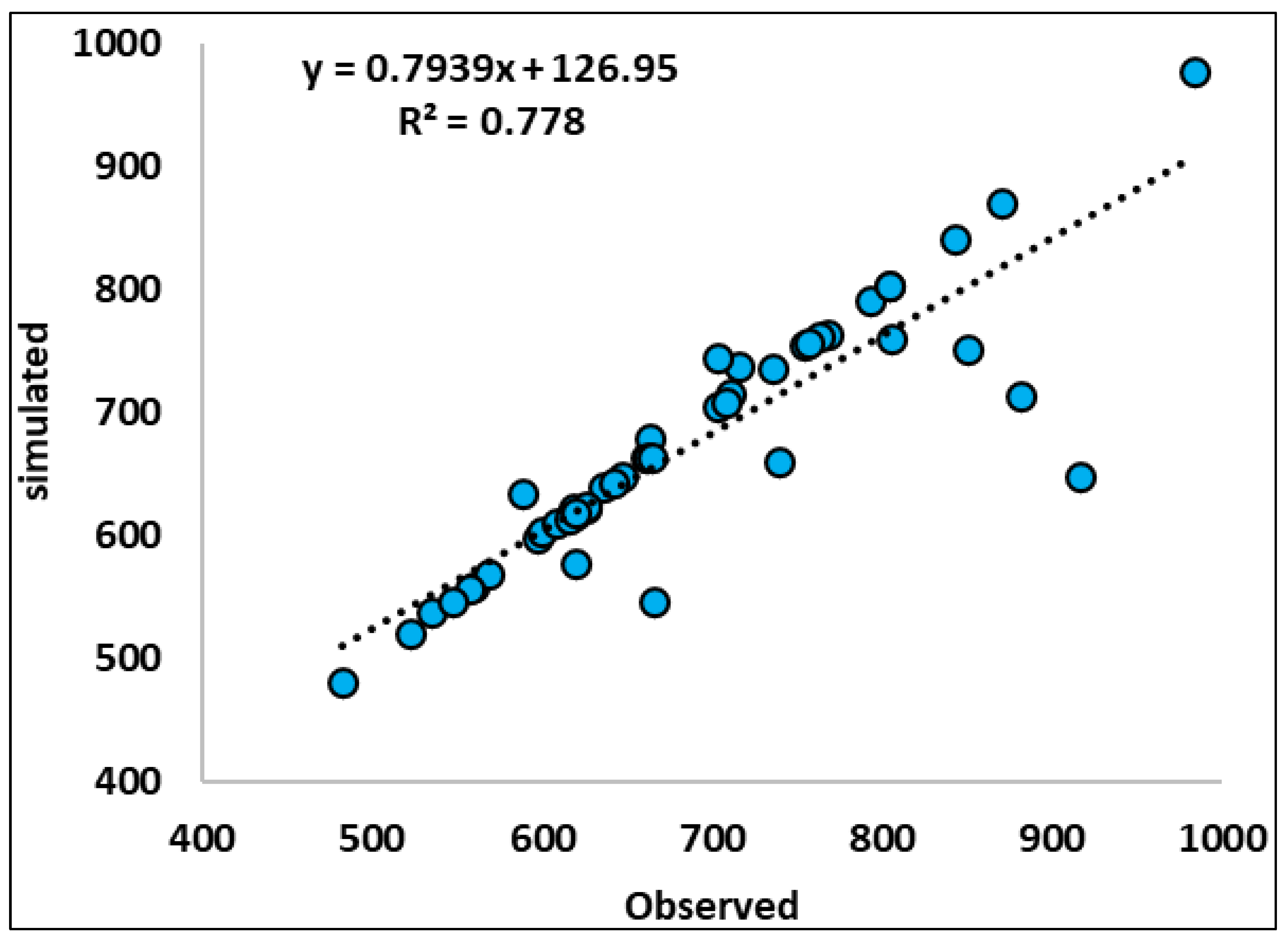
2.9. Measuring the Performance of the Model
2.10. Hurst Exponent Computation with Using of Rescale Range (R/S) Analysis Method
3. Results
3.1. Basic Statistics Analysis
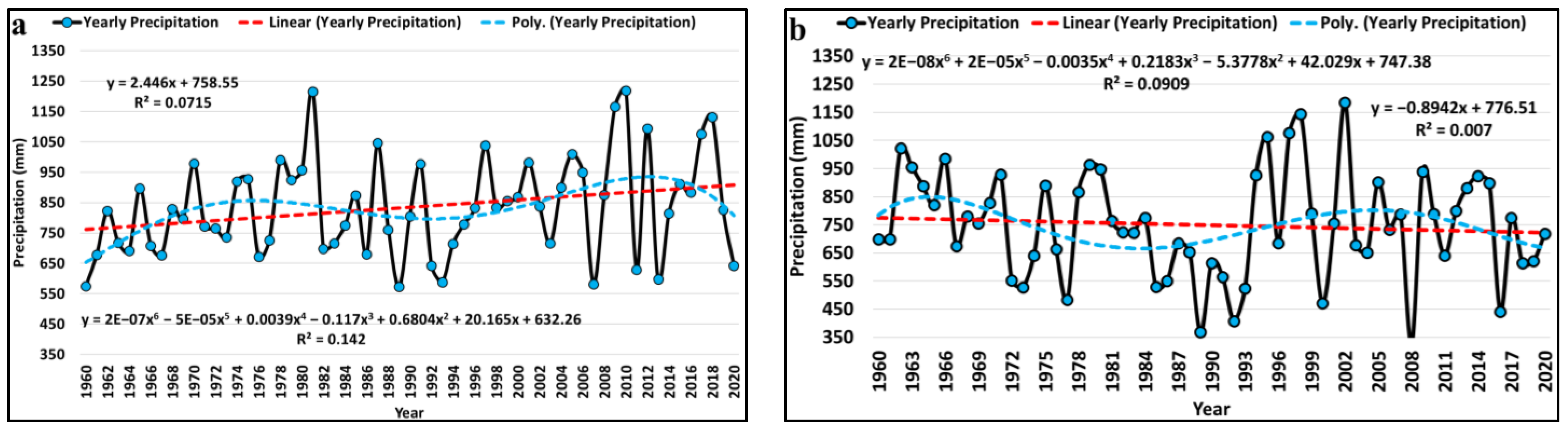
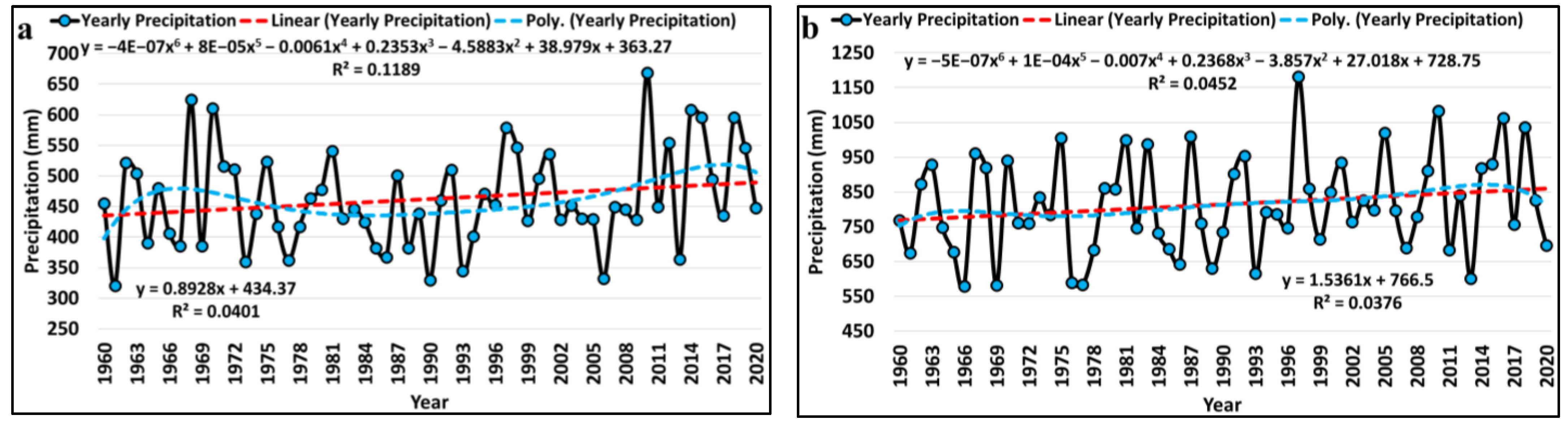
3.2. Time Series Analysis and Precipitation Situation in the Region
3.3. Man-Kendall Trend Analysis
3.4. Precipitation Distribution in the Study Area
3.4.1. Annual Precipitation Distribution
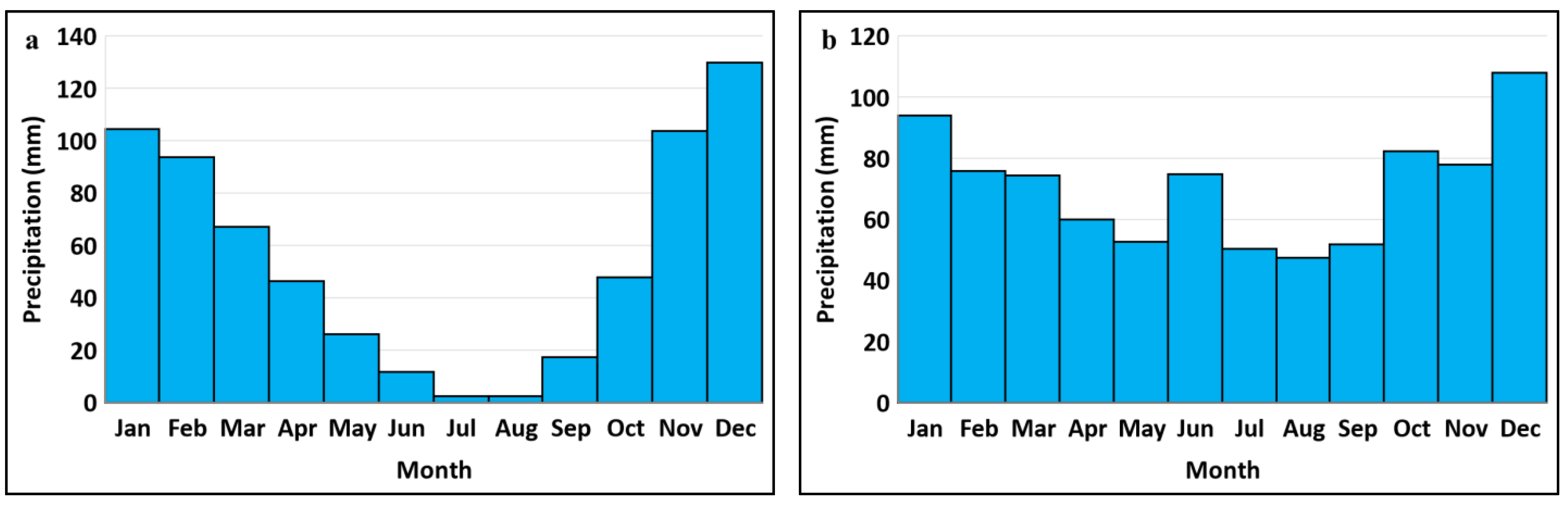
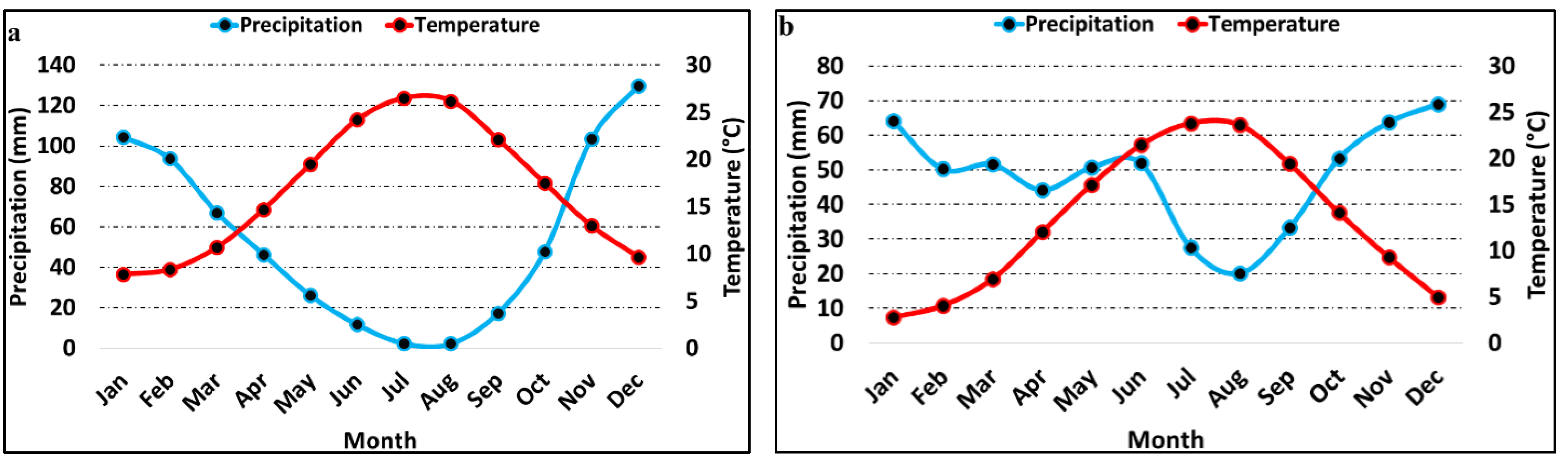
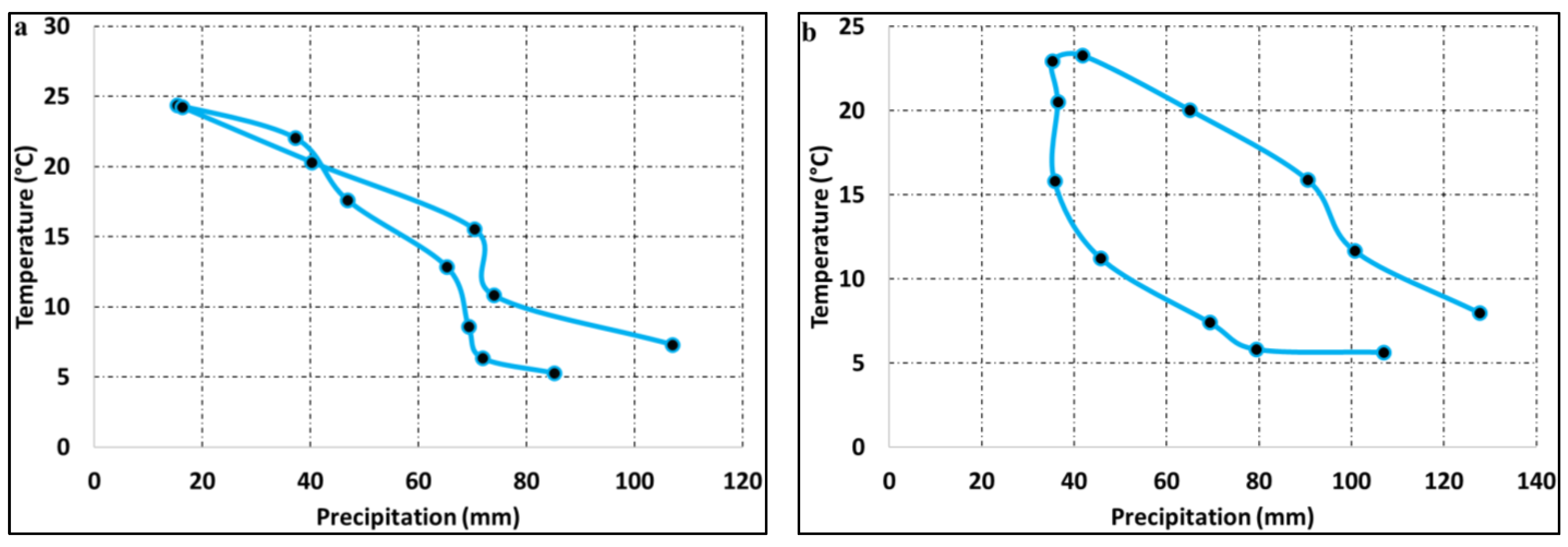
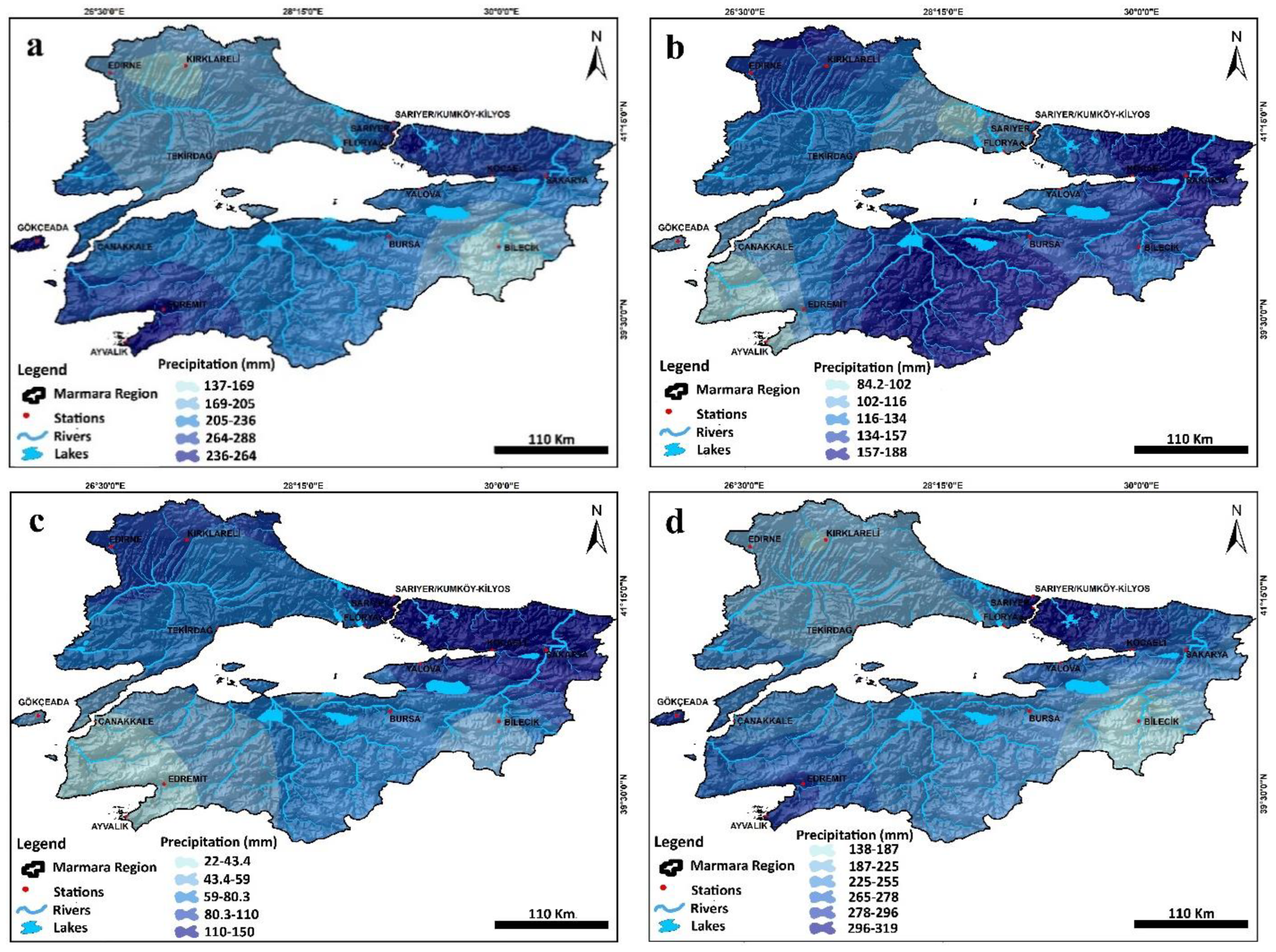
3.4.2. Seasonal Precipitation Distribution
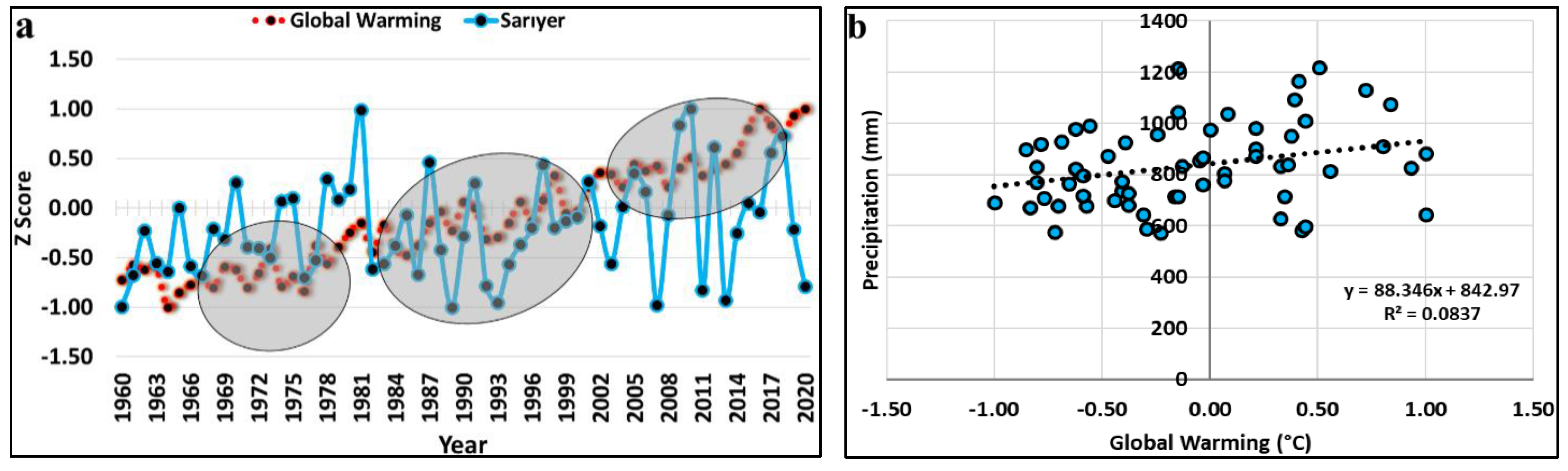
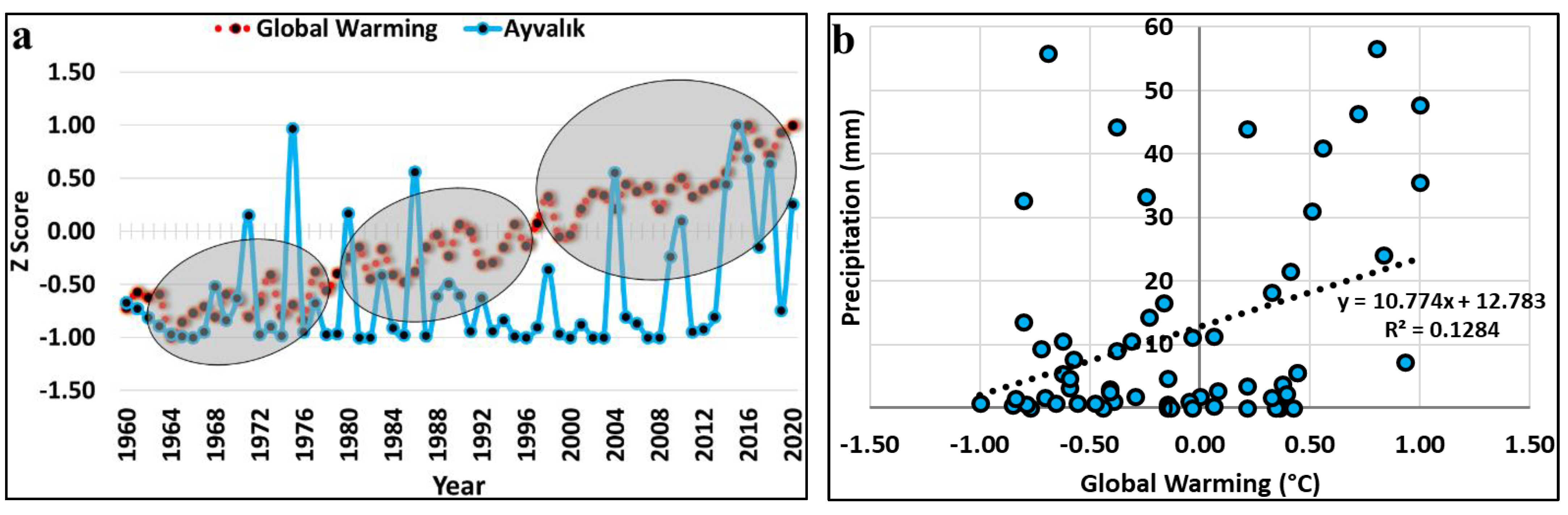
3.5. Exploring the Effects of GLOTI Index
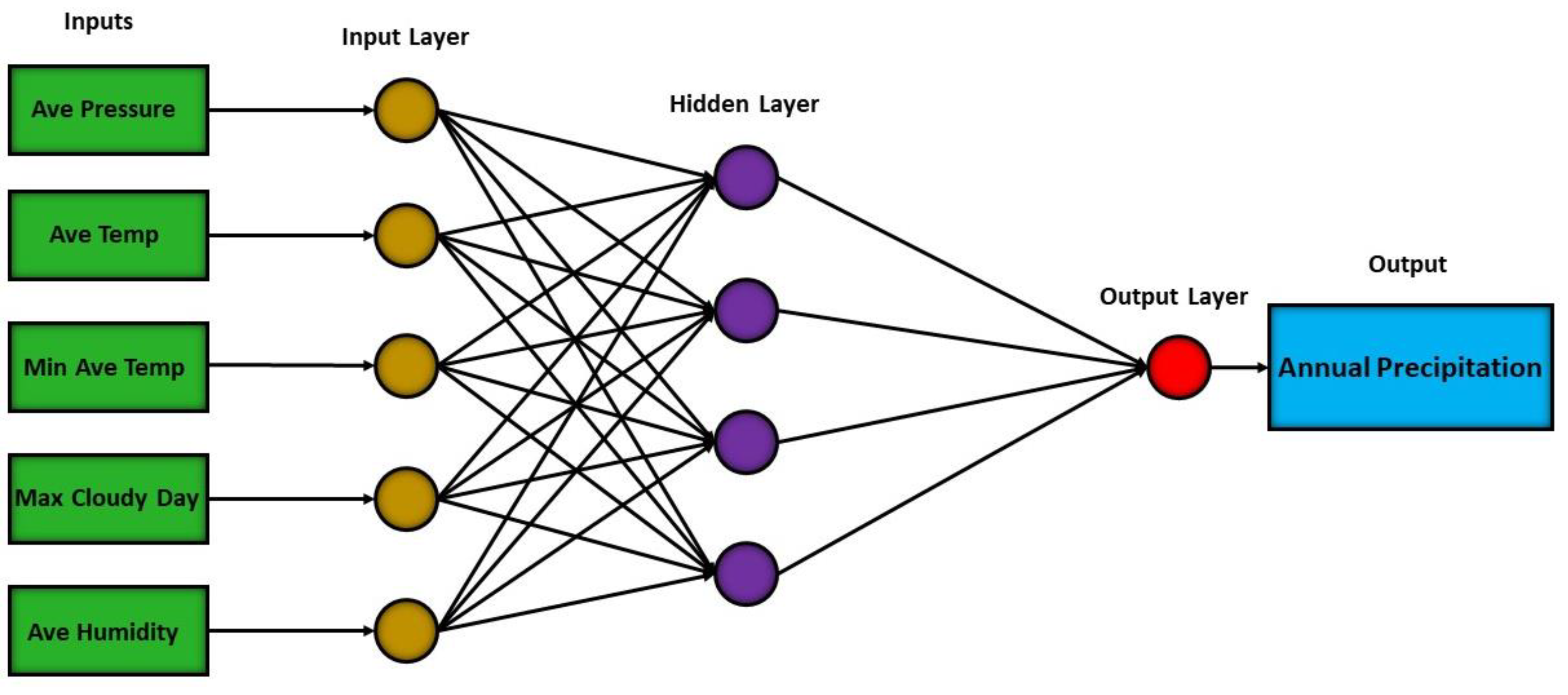
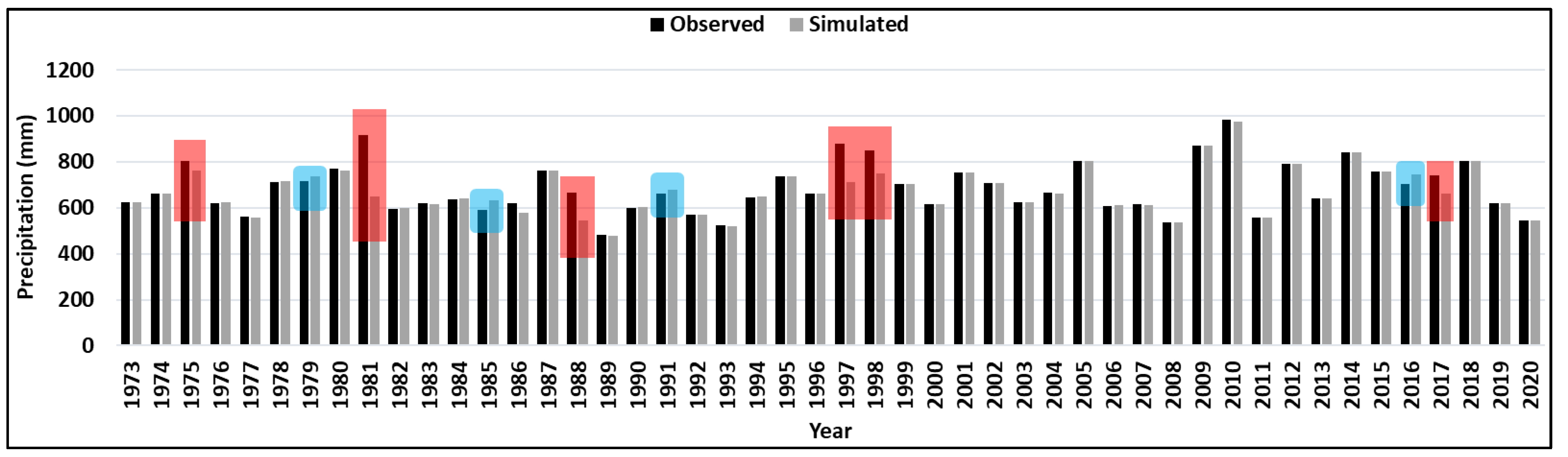
3.6. Precipitation Modeling with MLP-ANN
4. Discussion
5. Conclusions
Author Contributions
Funding
Institutional Review Board Statement
Informed Consent Statement
Data Availability Statement
Acknowledgments
Conflicts of Interest
References
- Frederick, K.D.; Major, D.C. Climate change and water resources. Clim. Chang. 1997, 37, 7–23. [Google Scholar] [CrossRef]
- Kansakar, S.R.; Hannah, D.M.; Gerrard, J.; Rees, G. Spatial pattern in the precipitation regime of Nepal. Int. J. Climatol. A J. R. Meteorol. Soc. 2004, 24, 1645–1659. [Google Scholar] [CrossRef]
- Xoplaki, E.; González-Rouco, J.F.; Luterbacher, J.; Wanner, H. Wet season Mediterranean precipitation variability: Influence of large-scale dynamics and trends. Clim. Dyn. 2004, 23, 63–78. [Google Scholar] [CrossRef] [Green Version]
- López-Díaz, F.; Conde, C.; Sánchez, O. Analysis of indices of extreme temperature events at Apizaco, Tlaxcala, Mexico: 1952–2003. Atmósfera 2013, 26, 349–358. [Google Scholar] [CrossRef] [Green Version]
- Chen, S.; Hu, J.; Zhang, A.; Min, C.; Huang, C.; Liang, Z. Performance of near real-time Global Satellite Mapping of Precipitation estimates during heavy precipitation events over northern China. Theor. Appl. Climatol. 2019, 135, 877–891. [Google Scholar] [CrossRef]
- Aalijahan, M.; Khosravichenar, A. A multimethod analysis for average annual precipitation mapping in the Khorasan Razavi Province (Northeastern Iran). Atmosphere 2021, 12, 592. [Google Scholar] [CrossRef]
- Aalijahan, M.; Lupo, A.R.; Salahi, B.; Rahimi, Y.G.; Asl, M.F. The long-term (142 years) spatiotemporal reconstruction and synoptic analysis of extreme low temperatures (−15 °C or lower) in the northwest region of Iran. Theor. Appl. Climatol. 2022, 147, 1415–1436. [Google Scholar] [CrossRef]
- Pachauri, R.K.; Reisinger, A. IPCC Fourth Assessment Report; IPCC: Geneva, Switzerland, 2007. [Google Scholar]
- Hartmann, D.L.; Klein Tank, A.M.G.; Rusticucci, M.; Alexander, L.V.; Brönnimann, S.; Charabi, Y.; Dentener, F.J.; Dlugokencky, E.J.; Easterling, D.R.; Kaplan, A.; et al. Observations: Atmosphere and surface. In Climate Change 2013 the Physical Science Basis: Working Group I Contribution to the Fifth Assessment Report of the Intergovernmental Panel on Climate Change; Cambridge University Press: Cambridge, UK, 2013; pp. 159–254. [Google Scholar]
- Allan, R.P.; Soden, B.J. Atmospheric warming and the amplification of precipitation extremes. Science 2008, 321, 1481–1484. [Google Scholar] [CrossRef] [Green Version]
- Min, S.K.; Zhang, X.; Zwiers, F.W.; Hegerl, G.C. Human contribution to more-intense precipitation extremes. Nature 2011, 470, 378–381. [Google Scholar] [CrossRef] [PubMed]
- Shiu, C.J.; Liu, S.C.; Fu, C.; Dai, A.; Sun, Y. How much do precipitation extremes change in a warming climate? Geophys. Res. Lett. 2012, 39. [Google Scholar] [CrossRef] [Green Version]
- Field, C.B.; Barros, V.; Stocker, T.F.; Dahe, Q. (Eds.) Managing the Risks of Extreme Events and Disasters to Advance Climate Change Adaptation: Special Report of the Intergovernmental Panel on Climate Change; Cambridge University Press: Cambridge, UK, 2012. [Google Scholar]
- Asadieh, B.; Krakauer, N.Y. Global trends in extreme precipitation: Climate models versus observations. Hydrol. Earth Syst. Sci. 2015, 19, 877–891. [Google Scholar] [CrossRef] [Green Version]
- Champion, A.J.; Blenkinsop, S.; Li, X.F.; Fowler, H.J. Synoptic-scale precursors of extreme UK summer 3-hourly rainfall. J. Geophys.Res. Atmos. 2019, 124, 4477–4489. [Google Scholar] [CrossRef]
- Margiorou, S.; Kastridis, A.; Sapountzis, M. Pre/Post-Fire Soil Erosion and Evaluation of Check-Dams Effectiveness in Mediterranean Suburban Catchments Based on Field Measurements and Modeling. Land 2022, 11, 1705. [Google Scholar] [CrossRef]
- Pastor, A.V.; Nunes, J.P.; Ciampalini, R.; Koopmans, M.; Baartman, J.; Huard, F.; Calheiros, T.; Le-Bissonnais, Y.; Keizer, J.J.; Raclot, D. Projecting future impacts of global change including fires on soil erosion to anticipate better land management in the forests of NW Portugal. Water 2019, 11, 2617. [Google Scholar] [CrossRef] [Green Version]
- Westra, S.; Alexander, L.V.; Zwiers, F.W. Global increasing trends in annual maximum daily precipitation. J. Clim. 2013, 26, 3904–3918. [Google Scholar] [CrossRef] [Green Version]
- Bocheva, L.; Pophristov, V. Seasonal analysis of large-scale heavy precipitation events in Bulgaria. In AIP Conference Proceedings; AIP Publishing LLC: Melville, NY, USA, 2019; Volume 2075, p. 200017. [Google Scholar]
- Solomon, S.; Manning, M.; Marquis, M.; Qin, D. Climate Change 2007-the Physical Science Basis: Working Group I Contribution to the Fourth Assessment Report of the IPCC; Cambridge University Press: Cambridge, UK, 2007; Volume 4. [Google Scholar]
- Pachauri, R.K.; Allen, M.R.; Barros, V.R.; Broome, J.; Cramer, W.; Christ, R.; Church, J.A.; Clarke, L.; Dahe, Q.; Dasgupta, P.; et al. Climate Change 2014: Synthesis Report. Contribution of Working Groups I, II and III to the Fifth Assessment Report of the Intergovernmental Panel on Climate Change; IPCC: Geneva, Switzerland, 2014; p. 151. [Google Scholar]
- Giorgi, F.; Lionello, P. Climate change projections for the Mediterranean region. Glob. Planet. Chang. 2008, 63, 90–104. [Google Scholar] [CrossRef]
- Palutikof, J.P.; Trigo, R.M.; Adcock, S.T. Scenarios of future rainfall over the Mediterranean: Is the region drying. In Proceedings of the Mediterranean Desertification, Research Results and Policy Implications, Crete, Greece, 29 October–1 November 1996; Volume 20, pp. 33–39. [Google Scholar]
- Piervitali, E.; Colacino, M.; Conte, M. Signals of climatic change in the central-western Mediterranean basin. Theor. Appl. Climatol. 1997, 58, 211–219. [Google Scholar] [CrossRef]
- Norrant, C.; Douguédroit, A. Monthly and daily precipitation trends in the Mediterranean (1950–2000). Theor. Appl. Climatol. 2006, 83, 89–106. [Google Scholar] [CrossRef]
- Philandras, C.M.; Nastos, P.T.; Kapsomenakis, J.; Douvis, K.C.; Tselioudis, G.; Zerefos, C.S. Long term precipitation trends and variability within the Mediterranean region. Nat. Hazards Earth Syst. Sci. 2011, 11, 3235–3250. [Google Scholar] [CrossRef] [Green Version]
- Alexandrov, V.; Schneider, M.; Koleva, E.; Moisselin, J.M. Climate variability and change in Bulgaria during the 20th century. Theor. Appl. Climatol. 2004, 79, 133–149. [Google Scholar] [CrossRef]
- Tomozeiu, R.; Stefan, S.; Busuioc, A. Winter precipitation variability and large-scale circulation patterns in Romania. Theor. Appl. Climatol. 2005, 81, 193–201. [Google Scholar] [CrossRef]
- Feidas, H.; Noulopoulou, C.; Makrogiannis, T.; Bora-Senta, E. Trend analysis of precipitation time series in Greece and their relationship with circulation using surface and satellite data: 1955–2001. Theor. Appl. Climatol. 2007, 87, 155–177. [Google Scholar] [CrossRef]
- Gönençgil, B.; İçel, G. Variations of total yearly precipitation in Eastern Mediterranean coasts of Turkey (1975–2006). Türk. Coğrafya Derg. 2010, 55, 2014. (In Turkish) [Google Scholar]
- Partal, T.; Kahya, E. Trend analysis in Turkish precipitation data. Hydrol. Process. Int. J. 2006, 20, 2011–2026. [Google Scholar] [CrossRef]
- Tayanç, M.; İm, U.; Doğruel, M.; Karaca, M. Climate change in Turkey for the last half century. Clim. Chang. 2009, 94, 483–502. [Google Scholar] [CrossRef]
- Türkeş, M. Spatial and temporal analysis of annual rainfall variations in Turkey. Int. J. Climatol. A J. R. Meteorol. Soc. 1996, 16, 1057–1076. [Google Scholar] [CrossRef]
- Özhan, S. Watershed Management; Publication No. 481; Istanbul University: Istanbul, Türkiye, 2004. (In Turkish) [Google Scholar]
- Atalay, I. Applied Climatology; META Basım Printing Services: Bornova, Türkiye, 2010. (In Turkish) [Google Scholar]
- Abbasnia, M.; Toros, H. Analysis of Long-Term Changes in Extreme Climatic Indices: A Case Study of the Mediterranean Climate, Marmara Region, Turkey. In Meteorology and Climatology of the Mediterranean and Black Seas; Springer Nature: Cham, Switzerland, 2019; pp. 141–153. [Google Scholar]
- Babai-Fini, O.M.; Najafpour, B. Climate Maps and Diagrams; Payam Noor University: Tehran, Iran, 2014. [Google Scholar]
- Farajzadeh Asl, M. Climatology Techniques; Samt: Tehran. Iran, 2015. (In Persian) [Google Scholar]
- Lanzante, J.R. Resistant, robust and non-parametric techniques for the analysis of climate data: Theory and examples, including applications to historical radiosonde station data. Int. J. Climatol. A J. R. Meteorol. Soc. 1996, 16, 1197–1226. [Google Scholar] [CrossRef]
- Davis, J.C.; Sampson, R.J. Statistics and Data Analysis in Geology; Wiley: New York, NY, USA, 1986; Volume 646. [Google Scholar]
- Rossi, R.E.; Mulla, D.J.; Journel, A.G.; Franz, E.H. Geostatistical tools for modeling and interpreting ecological spatial dependence. Ecol. Monogr. 1992, 62, 277–314. [Google Scholar] [CrossRef]
- Yadav, R.; Tripathi, S.K.; Pranuthi, G.; Dubey, S.K. Trend analysis by Mann-Kendall test for precipitation and temperature for thirteen districts of Uttarakhand. J. Agrometeorol. 2014, 16, 164. [Google Scholar] [CrossRef]
- Pohlert, T. Non-parametric trend tests and change-point detection. CC BY-ND 2016, 4, 1–18. [Google Scholar]
- Zaghloul, M.S.; Ghaderpour, E.; Dastour, H.; Farjad, B.; Gupta, A.; Eum, H.; Achari, G.; Hassan, Q.K. Long-Term Trend Analysis of River Flow and Climate in Northern Canada. Hydrology 2022, 9, 197. [Google Scholar] [CrossRef]
- Shawky, M.; Ahmed, M.R.; Ghaderpour, E.; Gupta, A.; Achari, G.; Dewan, A.; Hassan, Q.K. Remote sensing-derived land surface temperature trends over South Asia. Ecol. Inform. 2023, 74, 101969. [Google Scholar] [CrossRef]
- Li, L.J.; Zhang, L.; Wang, H.; Wang, J.; Yang, J.W.; Jiang, D.J.; Li, J.Y.; Qin, D.Y. Assessing the impact of climate variability and human activities on streamflow from the Wuding River basin in China. Hydrol. Process. Int. J. 2007, 21, 3485–3491. [Google Scholar] [CrossRef]
- Tian, F.; Yang, Y.; Han, S. Using runoff slope-break to determine dominate factors of runoff decline in Hutuo River Basin, North China. Water Sci. Technol. 2009, 60, 2135–2144. [Google Scholar] [CrossRef] [PubMed]
- Ye, X.; Zhang, Q.; Liu, J.; Li, X.; Xu, C.Y. Distinguishing the relative impacts of climate change and human activities on variation of streamflow in the Poyang Lake catchment, China. J. Hydrol. 2013, 494, 83–95. [Google Scholar] [CrossRef]
- Zhang, X.; Li, P.; Li, D. Spatiotemporal variations of precipitation in the southern part of the Heihe river basin (China), 1984–2014. Water 2018, 10, 410. [Google Scholar] [CrossRef] [Green Version]
- Efe, B.; Gözet, E.; Özgür, E.; Lupo, A.R.; Deniz, A. Spatiotemporal Variation of Tourism Climate Index for Türkiye during 1981–2020. Climate 2022, 10, 151. [Google Scholar] [CrossRef]
- Liu, J.; Xue, B.; Sun, W.; Guo, Q. Water balance changes in response to climate change in the upper Hailar River Basin, China. Hydrol. Res. 2020, 51, 1023–1035. [Google Scholar] [CrossRef]
- Feyzi, V. Analysis of Spatial-Temporal Distribution of Climate Change in Iran. Master’s Thesis, Faculty of Literature and Humanities, Department of Physical Geography, Tarbiat Modares University, Tehran, Iran, 2009. (In Persian). [Google Scholar]
- Wang, W.; Van Gelder, P.H.; Vrijling, J.K.; Ma, J. Forecasting daily streamflow using hybrid ANN models. J. Hydrol. 2006, 324, 383–399. [Google Scholar] [CrossRef]
- Alberto Meda-Campana, J. On the estimation and control of nonlinear systems with parametric uncertainties and noisy outputs. IEEE Access 2018, 6, 31968–31973. [Google Scholar] [CrossRef]
- Chiang, H.S.; Chen, M.Y.; Huang, Y.J. Wavelet-based EEG processing for epilepsy detection using fuzzy entropy and associative petri net. IEEE Access 2019, 7, 103255–103262. [Google Scholar] [CrossRef]
- Velasco LC, P.; Serquiña, R.P.; Zamad MS, A.A.; Juanico, B.F.; Lomocso, J.C. Performance analysis of multilayer perceptron neural network models in week-ahead rainfall forecasting. Int. J. Adv. Comput. Sci. Appl. 2019, 10, 578–588. [Google Scholar] [CrossRef] [Green Version]
- Elias, I.; Rubio, J.D.J.; Martinez, D.I.; Vargas, T.M.; Garcia, V.; Mujica-Vargas, D.; Meda-Campaña, J.A.; Pacheco, J.; Gutierrez, G.J.; Zacarias, A. Genetic algorithm with radial basis mapping network for the electricity consumption modeling. Appl. Sci. 2020, 10, 4239. [Google Scholar] [CrossRef]
- Ojo, O.S.; Adeyemi, B.; Oluleye, D.O. Artificial neural network models for prediction of net radiation over a tropical region. Neural Comput. Appl. 2021, 33, 6865–6877. [Google Scholar] [CrossRef]
- Ali, Z.; Hussain, I.; Faisal, M.; Nazir, H.M.; Hussain, T.; Shad, M.Y.; Mohamd Shoukry, A.; Hussain Gani, S. Forecasting drought using multilayer perceptron artificial neural network model. Adv. Meteorol. 2017, 2017, 5681308. [Google Scholar] [CrossRef] [Green Version]
- Luk, K.C.; Ball, J.E.; Sharma, A. A study of optimal model lag and spatial inputs to artificial neural network for rainfall forecasting. J. Hydrol. 2000, 227, 56–65. [Google Scholar] [CrossRef]
- Esteves, J.T.; de Souza Rolim, G.; Ferraudo, A.S. Rainfall prediction methodology with binary multilayer perceptron neural networks. Clim. Dyn. 2019, 52, 2319–2331. [Google Scholar] [CrossRef]
- Shah, H.; Ghazali, R. Prediction of earthquake magnitude by an improved ABC-MLP. In 2011 Developments in E-Systems Engineering; IEEE: New York, NY, USA, 2011; pp. 312–317. [Google Scholar]
- Yamany, W.; Tharwat, A.; Hassanin, M.F.; Gaber, T.; Hassanien, A.E.; Kim, T.H. A new multi-layer perceptrons trainer based on ant lion optimization algorithm. In Proceedings of the 2015 Fourth International Conference on Information Science and Industrial Applications (ISI), Busan, Republic of Korea, 20–22 September 2015; pp. 40–45. [Google Scholar]
- Miksovsky, J.; Raidl, A. Testing the performance of three nonlinear methods of time seriesanalysis for prediction and downscaling of European daily temperatures. Nonlinear Process. Geophys. 2005, 12, 979–991. [Google Scholar] [CrossRef] [Green Version]
- Hernández, G.; Zamora, E.; Sossa, H.; Téllez, G.; Furlán, F. Hybrid neural networks for big data classification. Neurocomputing 2020, 390, 327–340. [Google Scholar] [CrossRef]
- Faris, H.; Alkasassbeh, M.; Rodan, A. Artificial Neural Networks for Surface Ozone Prediction: Models and Analysis. Pol. J. Environ. Stud. 2014, 23, 341–348. [Google Scholar]
- Mukherjee, I.; Routroy, S. Comparing the performance of neural networks developed by using Levenberg–Marquardt and Quasi-Newton with the gradient descent algorithm for modelling a multiple response grinding process. Expert Syst. Appl. 2012, 39, 2397–2407. [Google Scholar] [CrossRef]
- Fletcher, R. Practical Methods of Optimization; John Wiley & Sons: Singapore, 2013. [Google Scholar]
- Asirvadam, V.S.; McLoone, S.F.; Irwin, G.W. Memory efficient BFGS neural-network learning algorithms using MLP-network: A survey. In Proceedings of the 2004 IEEE International Conference on Control Applications, Taipei, Taiwan, 2–4 September 2004; Volume 1, pp. 586–591. [Google Scholar]
- Hery, M.A.; Ibrahim, M.; June, L.W. BFGS method: A new search direction. Sains Malays. 2014, 43, 1591–1597. [Google Scholar]
- Sudheer, K.P.; Srinivasan, K.; Neelakantan, T.R.; Srinivas, V.V. A nonlinear data-driven model for synthetic generation of annual streamflows. Hydrol. Process. Int. J. 2008, 22, 1831–1845. [Google Scholar] [CrossRef]
- Vivekanandan, N. Prediction of rainfall using mlp and rbf networks. Int. J. Adv. Netw. Appl. 2014, 5, 1974. [Google Scholar]
- Chicco, D.; Warrens, M.J.; Jurman, G. The coefficient of determination R-squared is more informative than SMAPE, MAE, MAPE, MSE and RMSE in regression analysis evaluation. PeerJ Comput. Sci. 2021, 7, e623. [Google Scholar] [CrossRef]
- Valle, M.V.; García, G.M.; Cohen, I.S.; Klaudia Oleschko, L.; Ruiz Corral, J.A.; Korvin, G. Spatial variability of the Hurst exponent for the daily scale rainfall series in the state of Zacatecas, Mexico. J. Appl. Meteorol. Climatol. 2013, 52, 2771–2780. [Google Scholar] [CrossRef]
- Balkissoon, S.; Fox, N.; Lupo, A. Fractal characteristics of tall tower wind speeds in Missouri. Renew. Energy 2020, 154, 1346–1356. [Google Scholar] [CrossRef]
- Taqqu, M.S.; Teverovsky, V.; Willinger, W. Estimators for long-range dependence: An empirical study. Fractals 1995, 3, 785–798. [Google Scholar] [CrossRef]
- Kendziorski, C.M.; Bassingthwaighte, J.B.; Tonellato, P.J. Evaluating maximum likelihood estimation methods to determine the Hurst coefficient. Phys. A Stat. Mech. Its Appl. 1999, 273, 439–451. [Google Scholar] [CrossRef] [Green Version]
- Feng, L.; Zhou, J. Trend predictions in water resources using rescaled range (R/S) analysis. Environ. Earth Sci. 2013, 68, 2359–2363. [Google Scholar] [CrossRef]
- Tatli, H. Detecting persistence of meteorological drought via the Hurst exponent. Meteorol. Appl. 2015, 22, 763–769. [Google Scholar] [CrossRef]
- Pal, S.; Dutta, S.; Nasrin, T.; Chattopadhyay, S. Hurst exponent approach through rescaled range analysis to study the time series of summer monsoon rainfall over northeast India. Theor. Appl. Climatol. 2020, 142, 581–587. [Google Scholar] [CrossRef]
- Rao, A.R.; Bhattacharya, D. Comparison of Hurst exponent estimates in hydrometeorological time series. J. Hydrol. Eng. 1999, 4, 225–231. [Google Scholar] [CrossRef]
- Setty, V.A.; Sharma, A.S. Characterizing detrended fluctuation analysis of multifractional Brownian motion. Phys. A Stat. Mech. Its Appl. 2015, 419, 698–706. [Google Scholar] [CrossRef]
- Hurst, H.E. Long-term storage capacity of reservoirs. Trans. Am. Soc. Civ. Eng. 1951, 116, 770–808. [Google Scholar] [CrossRef]
- Kanounikov, I.E.; Antonova, E.V.; Kiselev, B.V.; Belov, D.R. Dependence of one of the fractal characteristics (Hurst exponent) of the human electroencephalogram on the cortical area and type of activity. In Proceedings of the IJCNN’99. International Joint Conference on Neural Networks. Proceedings (Cat. No. 99CH36339), Washington, DC, USA, 10–16 July 1999; Volume 1, pp. 243–246. [Google Scholar]
- Yurtseven, İ.; Serengil, Y. Changes and trends of seasonal total rainfall in the province of Istanbul, Turkey. J. Fac. For. Istanb. Univ. 2017, 67, 1–12. [Google Scholar] [CrossRef] [Green Version]
- Caloiero, T.; Caloiero, P.; Frustaci, F. Long-term precipitation trend analysis in Europe and in the Mediterranean basin. Water Environ. J. 2018, 32, 433–445. [Google Scholar] [CrossRef]
- Kastridis, A.; Kamperidou, V.; Stathis, D. Dendroclimatological Analysis of Fir (A. borisii-regis) in Greece in the frame of Climate Change Investigation. Forests 2022, 13, 879. [Google Scholar] [CrossRef]
- Mersin, D.; Tayfur, G.; Vaheddoost, B.; Safari, M.J.S. Historical trends associated with annual temperature and precipitation in Aegean Turkey, where are we heading? Sustainability 2022, 14, 13380. [Google Scholar] [CrossRef]
- Todaro, V.; D’Oria, M.; Secci, D.; Zanini, A.; Tanda, M.G. Climate change over the Mediterranean region: Local temperature and precipitation variations at five pilot sites. Water 2022, 14, 2499. [Google Scholar] [CrossRef]
- Varlas, G.; Stefanidis, K.; Papaioannou, G.; Panagopoulos, Y.; Pytharoulis, I.; Katsafados, P.; Papadopoulos, A.; Dimitriou, E. Unravelling precipitation trends in Greece since 1950s using ERA5 climate reanalysis data. Climate 2022, 10, 12. [Google Scholar] [CrossRef]
- Bacanli, U.G.; Tanrikulu, A. Trends in Yearly Precipitation and Temperature on the Aegean Region, Turkey. In Ovidius University Annals, Series Civil Engineering; Ovidius University Press: Constanța, Romania, 2016; Volume 18. [Google Scholar]
- Güner Bacanli, Ü. Trend analysis of precipitation and drought in the A egean region, Turkey. Meteorol. Appl. 2017, 24, 239–249. [Google Scholar] [CrossRef]
- Abu Hammad, A.H.; Salameh, A.A.; Fallah, R.Q. Precipitation Variability and Probabilities of Extreme Events in the Eastern Mediterranean Region (Latakia Governorate-Syria as a Case Study). Atmosphere 2022, 13, 131. [Google Scholar] [CrossRef]
- Balcıoğlu, Y.E.; Gönençgil, B. Trends of temperature and precipitation in the north and south of İstanbul as a transitional climate zone. In Proceedings of the TÜCAUM 2022 International Geography Symposium, Ankara, Turkey, 12–14 October 2022. [Google Scholar]
- Drori, R.; Ziv, B.; Saaroni, H.; Etkin, A.; Sheffer, E. Recent changes in the rain regime over the Mediterranean climate region of Israel. Clim. Chang. 2021, 167, 15. [Google Scholar] [CrossRef]
- Lionello, P.; Malanotte-Rizzoli, P.; Boscolo, R.; Alpert, P.; Artale, V.; Li, L.; Luterbacher, J.; May, W.; Trigo, R.; Tsimplis, M.; et al. The Mediterranean climate: An overview of the main characteristics and issues. Dev. Earth Environ. Sci. 2006, 4, 1–26. [Google Scholar]
- Türkeş, M.; Deniz, Z.A. Climatology of South Marmara Division (North West Anatolia) and observed variations and trends. J. Hum. Sci. 2011, 8, 1579–1600. [Google Scholar]
- Asikoglu, O.L.; Ciftlik, D. Recent rainfall trends in the Aegean region of Turkey. J. Hydrometeorol. 2015, 16, 1873–1885. [Google Scholar] [CrossRef]
- Çağlıyan, A.; Gülsen, A. Spatial analysis of precipitation in Turkey. In Proceedings of the International Geography Symposium on the 30th Anniversary of TUCAUM, Ankara, Türkiye, 3–6 October 2018. [Google Scholar]
- Atalay, I.; Efe, R. Structural and distributional evaluation of forest ecosystems in Türkiye. J. Environ. Biol. 2010, 31, 61. [Google Scholar]
- Atalay, I. Climate Atlas of Turkey; İnkılap Publishing House: Istanbul, Türkiye, 2011. (In Turkish) [Google Scholar]
- Bilgili, M.; Sahin, B. Prediction of long-term monthly temperature and rainfall in Turkey. Energy Sources Part A 2009, 32, 60–71. [Google Scholar] [CrossRef]
- Moustris, K.P.; Larissi, I.K.; Nastos, P.T.; Paliatsos, A.G. Precipitation forecast using artificial neural networks in specific regions of Greece. Water Resour. Manag. 2011, 25, 1979–1993. [Google Scholar] [CrossRef]
- Yıldıran, A.; Yerel Kandemir, S. Prediction of Precipitation with Artificial Neural Networks. Bilecik Şeyh Edebali Univ. J. Sci. 2018, 5, 97–104. [Google Scholar]
- Estevez, J.; Liu, X.; Bellido-Jimenez, J.A.; Garcia-Marin, A.P. Assessing Wavelet Analysis for Precipitation Forecasts Using Artificial Neural Networks in Mediterranean Coast. In Proceedings of the ITISE 2019, Granada, Spain, 25–27 September 2019; Volume 2. [Google Scholar]
- Elbeltagi, A.; Zerouali, B.; Bailek, N.; Bouchouicha, K.; Pande, C.; Santos, C.A.G.; Towfiqul Islam, A.R.M.; Al-Ansari, N.; El-kenawy, E.S.M. Optimizing hyperparameters of deep hybrid learning for rainfall prediction: A case study of a Mediterranean basin. Arab. J. Geosci. 2022, 15, 933. [Google Scholar] [CrossRef]


| Row | Station No | Station | Altitude (m) | Latitude (Degree) | Longitude (Degree) |
|---|---|---|---|---|---|
| 1 | 17,175 | Ayvalık | 4 | 39.3113 | 26.6861 |
| 2 | 17,120 | Bilecik | 539 | 40.1414 | 29.9772 |
| 3 | 17,116 | Bursa | 100 | 40.2308 | 29.0133 |
| 4 | 17,112 | Çanakkale | 6 | 40.141 | 26.3993 |
| 5 | 17,050 | Edirne | 51 | 41.6767 | 26.5508 |
| 6 | 17,145 | Edremit | 21 | 39.5895 | 27.0192 |
| 7 | 17,636 | Florya | 37 | 40.9758 | 28.7865 |
| 8 | 17,110 | Gökçeada | 79 | 40.191 | 25.9075 |
| 9 | 17,052 | Kırklareli | 232 | 41.7382 | 27.2178 |
| 10 | 17,066 | Kocaeli | 74 | 40.7663 | 29.9173 |
| 11 | 17,059 | Sarıyer/Kumköy-Kilyos | 38 | 41.2505 | 29.0384 |
| 12 | 17,069 | Sakarya | 30 | 40.7676 | 30.3934 |
| 13 | 17,061 | Sarıyer | 59 | 41.1464 | 29.0502 |
| 14 | 17,056 | Tekirdağ | 4 | 40.9585 | 27.4965 |
| 15 | 17,119 | Yalova | 4 | 40.6589 | 29.2796 |
| Station | Mean (mm) | Std. Deviation (mm) | Minimum (mm) | Maximum (mm) | Range (mm) | CV (%) |
|---|---|---|---|---|---|---|
| Ayvalık | 652.70 | 140.90 | 304.60 | 992.30 | 687.70 | 0.22 |
| Bilecik | 462.10 | 79.20 | 320.40 | 668.70 | 348.30 | 0.17 |
| Bursa | 698.60 | 139.50 | 446.40 | 1328.20 | 881.80 | 0.20 |
| Çanakkale | 615.60 | 137.90 | 343.90 | 977.70 | 633.80 | 0.22 |
| Edirne | 601.70 | 129.00 | 387.00 | 958.60 | 571.60 | 0.21 |
| Edremit | 700.00 | 174.10 | 377.00 | 1220.30 | 843.30 | 0.25 |
| Florya | 643.80 | 122.60 | 420.10 | 969.10 | 549.00 | 0.19 |
| Gökçeada | 748.80 | 189.40 | 326.00 | 1185.10 | 859.10 | 0.25 |
| Kırklareli | 580.10 | 142.00 | 326.60 | 990.30 | 663.70 | 0.24 |
| Kocaeli | 814.10 | 140.60 | 579.30 | 1180.80 | 601.50 | 0.17 |
| Kumköy-Kilyos | 807.60 | 170.40 | 470.60 | 1231.20 | 760.60 | 0.21 |
| Sakarya | 849.70 | 139.30 | 600.70 | 1268.50 | 667.80 | 0.16 |
| Sarıyer | 834.40 | 162.30 | 574.20 | 1218.80 | 644.60 | 0.19 |
| Tekirdağ | 579.90 | 132.80 | 334.60 | 896.30 | 561.70 | 0.23 |
| Yalova | 745.80 | 154.00 | 472.40 | 1293.20 | 820.80 | 0.21 |
| Station | Jan | Feb | Mar | Apr | May | Jun | Jul | Aug | Sep | Oct | Nov | Dec | Annually |
|---|---|---|---|---|---|---|---|---|---|---|---|---|---|
| Ayvalık | 0.122 | 0.010 | −0.187 | −0.041 | −0.020 | 0.358 ** | 0.113 | −0.048 | −0.026 | 0.347 ** | 0.023 | −0.170 | 0.085 |
| Bilecik | 0.063 | 0.154 | −0.012 | −0.022 | −0.049 | 0.335 ** | −0.040 | −0.188 | 0.116 | 0.177 | −0.113 | −0.016 | 0.220 |
| Bursa | 0.020 | 0.081 | 0.050 | −0.025 | 0.171 | 0.272 * | −0.007 | −0.200 | 0.153 | 0.225 | −0.155 | −0.176 | 0.123 |
| Çanakkale | −0.039 | 0.066 | −0.039 | 0.036 | −0.068 | 0.208 | −0.088 | −0.109 | −0.076 | 0.185 | −0.010 | −0.183 | −0.043 |
| Edirne | 0.161 | 0.062 | 0.048 | −0.039 | 0.078 | 0.013 | 0.209 | −0.192 | 0.013 | 0.286 * | −0.034 | −0.059 | 0.183 |
| Edremit | 0.094 | 0.011 | −0.057 | −0.036 | −0.079 | 0.098 | 0.095 | −0.152 | −0.027 | 0.304 * | 0.031 | −0.189 | 0.018 |
| Florya | −0.021 | 0.150 | 0.007 | −0.148 | 0.128 | 0.121 | 0.045 | −0.112 | 0.091 | 0.116 | −0.088 | −0.194 | 0.000 |
| Gökçeada | 0.087 | −0.203 | 0.007 | 0.045 | 0.085 | 0.186 | −0.081 | 0.006 | −0.007 | 0.197 | −0.040 | −0.128 | −0.011 |
| Kırklareli | 0.079 | 0.024 | −0.082 | −0.179 | 0.092 | 0.186 | 0.205 | −0.153 | 0.166 | 0.266 * | −0.014 | −0.106 | 0.139 |
| Kocaeli | 0.228 | 0.122 | 0.065 | 0.005 | 0.218 | 0.234 | 0.204 | −0.004 | −0.051 | 0.056 | −0.100 | 0.003 | 0.274 * |
| Kumköy-Kilyos | −0.049 | 0.134 | −0.054 | −0.060 | 0.005 | 0.079 | 0.202 | −0.122 | 0.276 * | 0.095 | 0.037 | −0.065 | 0.131 |
| Sakarya | 0.156 | 0.124 | −0.033 | 0.017 | 0.303 * | 0.172 | 0.051 | −0.067 | −0.009 | 0.091 | −0.141 | 0.012 | 0.208 |
| Sarıyer | 0.049 | 0.216 | 0.026 | −0.145 | 0.065 | 0.288 * | 0.127 | −0.032 | 0.245 | 0.154 | 0.074 | −0.031 | 0.289 * |
| Tekirdağ | −0.081 | 0.146 | −0.148 | −0.072 | −0.006 | 0.021 | 0.210 | −0.126 | 0.087 | 0.274 * | −0.133 | −0.142 | 0.021 |
| Yalova | −0.010 | −0.110 | −0.086 | −0.116 | 0.223 | 0.170 | −0.084 | −0.005 | 0.029 | 0.198 | 0.020 | −0.109 | 0.043 |
| Row | Pressure | Humid | Cloud Cover | Sunshine | Temperature | Wind |
|---|---|---|---|---|---|---|
| 1 | Average | Average | Average | Monthly-Sum | Average | Average |
| 2 | Maximum | Maximum | Maximum | Daily Sum-Monthly Ave | Maximum | - |
| 3 | Minimum | Minimum | Minimum | - | Minimum | - |
| 4 | - | Ave-Max | - | - | Ave-Max | - |
| 5 | - | Ave-Min | - | - | Ave-Min | - |
| Variables | Ave-Pressure | Ave-Temp | Min/Ave-Temp | Max-Cloud | Ave-Humid |
|---|---|---|---|---|---|
| Correlation | −0.482 ** | 0.28 * | 0.312 * | 0.281 * | 0.301 * |
| Name | Hidden Layer | Number of Neuron | Training Algorithm | Error Function | Hidden Activation | Output Activation |
|---|---|---|---|---|---|---|
| MLP | 1 | 4 | BFGS | SOS | Exponential | Tanh |
Disclaimer/Publisher’s Note: The statements, opinions and data contained in all publications are solely those of the individual author(s) and contributor(s) and not of MDPI and/or the editor(s). MDPI and/or the editor(s) disclaim responsibility for any injury to people or property resulting from any ideas, methods, instructions or products referred to in the content. |
© 2023 by the authors. Licensee MDPI, Basel, Switzerland. This article is an open access article distributed under the terms and conditions of the Creative Commons Attribution (CC BY) license (https://creativecommons.org/licenses/by/4.0/).
Share and Cite
Aalijahan, M.; Karataş, A.; Lupo, A.R.; Efe, B.; Khosravichenar, A. Analyzing and Modeling the Spatial-Temporal Changes and the Impact of GLOTI Index on Precipitation in the Marmara Region of Türkiye. Atmosphere 2023, 14, 489. https://doi.org/10.3390/atmos14030489
Aalijahan M, Karataş A, Lupo AR, Efe B, Khosravichenar A. Analyzing and Modeling the Spatial-Temporal Changes and the Impact of GLOTI Index on Precipitation in the Marmara Region of Türkiye. Atmosphere. 2023; 14(3):489. https://doi.org/10.3390/atmos14030489
Chicago/Turabian StyleAalijahan, Mehdi, Atilla Karataş, Anthony R. Lupo, Bahtiyar Efe, and Azra Khosravichenar. 2023. "Analyzing and Modeling the Spatial-Temporal Changes and the Impact of GLOTI Index on Precipitation in the Marmara Region of Türkiye" Atmosphere 14, no. 3: 489. https://doi.org/10.3390/atmos14030489