ENSO and PDO Effect on Stratospheric Dynamics in Isca Numerical Experiments

Abstract

The deterministic forecast of the stratospheric polar vortex intensity (iSPV) is limited by 2 weeks, but it can be probabilistically predicted for a longer period due to low-frequency components of the climate system, such as large-scale sea surface temperature anomalies (SSTAs) (e.g., El Niño Southern Oscillation (ENSO) and Pacific Decadal Oscillation (PDO)). For a qualitative and quantitative assessment of the effect of the large-scale Pacific SSTAs on the iSPV anomalies formation, idealized model experiments were carried out using the Isca platform. There is no statistically significant response of the SPV dynamics to the SSTAs corresponding to PDO phases, but they noticeably correct the effect of ENSO modes when added to it. The effect of the El Niño (EN) and La Niña (LN) events with neutral PDO phases on the iSPV is asymmetric; in the “single” EN experiment the vortex is 40% weaker relative to the control values, and, in the “single” LN, the SPV is weakened by no more than 20%. When EN accompanied with the positive PDO phase, iSPV is reduced by 58%. When the negative PDO phase is added, the EN effect is significantly weakened. The LN effect is weakened by both positive and negative PDO phases.

1. Introduction

The stratosphere has a prognostic potential for weather forecasting on sub-seasonal time scales [1,2,3,4,5]. These time scales are considered to be a so-called predictability “grey zone” for which the predictions are highly inaccurate [6,7]. The extreme states of the stratospheric polar vortex (SPV) affect the location of the Northern Hemisphere storm tracks on the periods from 10 days to 2 months [2,8,9,10,11,12,13,14,15,16,17,18,19], thus providing potential predictability for mid-latitudinal states of the troposphere. This causes diagnostics and understanding the mechanisms of SPV variability to be crucial for predications of the troposphere dynamics. At present, the deterministic predictability of the stratospheric processes is limited by 1–2 weeks [20,21,22]. However, probabilistic predictions are possible for longer periods if they account for low-frequency components of the climate system; for example, large-scale sea surface temperature (SST) anomalies [23]. Natural modes of SST variability, such as the El Niño Southern Oscillation (ENSO) and the Pacific Decadal Oscillation (PDO), are predicted for up to 6 years [24,25]. The understanding of the formation of the SPV intensity anomalies in response to large-scale SST anomalies would lead to refining and expanding both weather and climate forecasts on the timescales from a season to decades.

During the El Niño years, the polar vortex tends to weaken [26,27]. The observational diagnostics and model experiments show that during El Niño events the Aleutian Low deepens, implying intensification of the Pacific-North American mode. This region is co-located with the mean climatological position of the trough of the quasi-stationary planetary wave 1. This wave is amplified here concurrently with the intensification of the vertical wave activity propagation into the stratosphere [28], which perturbs and weakens the vortex. This is also reflected in the Brewer–Dobson circulation strengthening [29,30]. Additionally, it was shown that the El Niño Modoki forms two Walker cells contrasting the canonical El Niño with the convection areas being formed in different parts of the Pacific Ocean [31,32] and affecting the troposphere-stratosphere interaction processes. Quasi-biennial oscillation (QBO) also strongly affects the propagation of quasi-stationary planetary waves correcting the effect of El Niño. The authors of [33] showed that, according to the observational data during La Niña and the neutral phase of the ENSO, the vortex in the eastern QBO is weaker than in the western QBO, but no such tendencies were found for the El Niño years.

The impact of the mid-latitude SST anomalies on the tropospheric dynamics is smaller compared to internal atmospheric variability [34] but may lead to a change in the probability distribution of some large-scale troposphere variability characteristics. Since only waves with small wave numbers propagate into the stratosphere from the troposphere, a kind of signal filtering occurs; the footprints of the mid-latitudes’ SST anomalies impact can be found in the characteristics of the stratospheric dynamics.

In [35,36,37,38,39], the effect of PDO on the SPV intensity were investigated. A weakened vortex is more often observed during the positive phase of the PDO [37]. When there are positive SST anomalies in the central Pacific Ocean in mid-latitudes, the polar stratosphere is warmer, but these works analyze the PDO index from observational data and cannot accurately separate the ENSO effect from the PDO effect. The model experiments [36] demonstrated that the warm North Pacific Ocean (negative PDO phase) leads to a less disturbed vortex on a seasonal scale. The authors of [35,40] showed that, in the negative PDO phase, the intensity of the vertical propagation of wave 1 can be a predictor of the SPV intensity on a monthly time scale, and, in the positive PDO phase, this does not occur.

The authors of [41] showed that the response in the North American region to changes in the meridional SST gradient is higher than to changes in the zonal SST characteristics. Previously, it was shown that an increase in the meridional SST gradient is associated with also increasing the meridional gradient in the tropical troposphere. The zonal wind in the upper troposphere intensifies due to the thermal wind balance, which in turn leads to an intensification of the planetary wave’s propagation into the polar region [42,43].

Some works investigate the combined effects of the ENSO and the PDO [44], but they are primarily based on the analysis of the observational data, in which the analysis of different factors is complicated.

All these results suggest that PDO has a significant impact on the dynamics of the troposphere and stratosphere through the transformation of the spatial structure and the intensity of the quasi-stationary planetary wave propagation. The major mechanisms are associated with the change of the meridional temperature gradient, with a local effect on baroclinicity, synoptic eddies, and the mean flow interaction.

Thus, for now, we do not have quantitative estimates of the impact of the large-scale SST anomalies on stratospheric dynamics. Additionally, no predictors of the SPV intensity anomalies formation under various boundary conditions, such as the ENSO and the PDO, have been identified.

The main goal of this work is to investigate the physical processes behind the effect of large-scale SST anomalies in the tropical and extratropical zones of the Pacific Ocean on the SPV intensity using the idealized modeling. These experiments do not reflect the influence of the PDO as a complex process of interaction between the ocean and the atmosphere with feedbacks [45,46] but, rather, the influence of SST anomalies in various regions of the Pacific Ocean.

2. Materials and Methods

2.1. Datasets

The merged dataset (Merged Hadley-NOAA/OI SST & SIC) [47], which consists of data from the Hadley Center of the Met Office (HadISST1) [48] and data with optimal interpolation from the National Oceanic and Atmospheric Administration (NOAA Optimal Interpolation v2) [49], was used for constructing the boundary conditions for the model experiments. The AMIP climatology data [50], which are represented by monthly average fields, were chosen as the climatological mean values of the SST and sea ice concentration data. The JRA-55 reanalysis data [51] were used to validate the model and assess the reliability of the reconstruction of the processes of the stratosphere-troposphere interaction obtained during the numerical experiments.

2.2. Isca Model

The idealized model experiments were performed using the Isca framework [52] to quantify the effect of the large-scale Pacific SST anomalies on the SPV variability through large-scale quasi-stationary planetary waves dynamics.

Isca is a framework for the idealized modeling of the global circulation of planetary atmospheres at varying levels of complexity and realism with the GFDL model as the dynamical core. The following model configuration was used in this work. The horizontal spectral resolution was T42 and the vertical resolution of the model was 40 levels, 18 of which were above the tropopause. The top of the model was a “sponge” layer at level of ~73 km (0.02 hPa), while the lower boundary of the dissipative layer was at a level of 150 Pa. The T42 ERA-Interim land mask and topography were used as the orography [53].

The same parametrizations as in [54] were used: radiative transfer: RRTM; moisture transformation: Bets-Miller convection scheme, Monin-Obukhov boundary layer scheme, mixed layer ocean, and large-scale condensation. Ozone is a key element in the processes of stratospheric heating and is important for reproducing the dynamics of atmospheric layers above 20 km and its variability can significantly affect the SPV dynamics. Therefore, in the experiments, a constant zonally symmetric ozone distribution was used, which was created from the CIRA datasets and observations from radiosondes [55,56].

In this work, we conducted “single” experiments with SST anomalies associated with El Niño (EN), La Niña (LN), positive phase of the PDO (PDO+), negative PDO phase (PDO−), and “merged” experiments: El Niño and positive PDO phase (EN&PDO+), El Niño and negative PDO phase (EN&PDO−), La Niña and positive PDO phase (LN&PDO+), and La Niña and negative PDO phase (LN&PDO−) (

Table 1. Table of experiments.

Boundary Conditions		Pacific Decadal Oscillation
		Neutral	Positive Phase	Negative Phase
ENSO	Neutral	+ (control)	+	+
	El Niño	+	+	+
	La Niña	+	+	+

). To validate the model and estimate the effect of the large-scale SST anomalies on the SPV dynamics, a control experiment (CTRL) was conducted, which had the same model configuration as in the experiments on the sensitivity of the dynamics of the stratosphere-troposphere interaction to large-scale Pacific Ocean SST anomalies. The climatological mean AMIP SST data were used as the boundary conditions in the control experiment. The duration of each experiment was 100 years.

2.3. Experiments Boundary Condition

The specific SST fields were created as boundary conditions. Doubled SST anomalies, corresponding to certain modes of the SST large-scale variability in the Pacific Ocean, in various combinations were added to the AMIP climatological mean values for each month in a year.

The El Niño Southern Oscillation (ENSO) is the most powerful SST oscillation in the World Ocean with amplitudes reaching 5–6 °C. In this work, the El Niño anomalies in the Nino-3 region were used [57,58,59].

Algorithm for constructing SST fields for boundary conditions:

• According to the calendars in the works [57,58], the years with events of maximum intensity were selected: for El Niño—1997/1998, and for La Niña—1975/1976. The algorithm used in [57,58] for selecting extreme events years coincides with that presented [60].
• The SST values in the region [20° N–20° S, 140° E–80° W] (EN region) were extracted from the monthly mean field of the SST anomalies for the selected years.
• The values in this region have been doubled and added to the climatological mean monthly SST values from AMIP data (Equation (1)).

$${\mathrm{SST}}_{\exp }={ \mathrm{SST}}_{\mathrm{AMIP}}+2 {\ast \mathrm{anSST}}_{\mathrm{ENSO}/\mathrm{PDO}}$$

(1)

Since the anomalies along the border of the EN region are almost equal to zero, doubling them did not lead to the appearance of sharp gradients (Figure S1).

Similarly, the SST fields corresponding to the Pacific Decadal Oscillation, one of the most extended SST anomalies in the mid-latitudes of the Northern Hemisphere in the World Ocean, were obtained.

• The PDO index was calculated as the principal component of the first empirical orthogonal function of the SST anomalies in the northern part of the Pacific Ocean [61,62] for the region [20° N–60° N, 120° E–250° E] (Figure S2).
• The years with the maximum and minimum values of the PDO index were determined: for the positive phase, it is 1949, while, for the negative phase, it is 1941.
• For the above-mentioned area, the SST anomalies were doubled and added to the climatological mean AMIP SST fields (Figure S3).

2.4. Analysis Methods

The Fourier method was used to analyze the amplitudes and phases of quasi-stationary planetary waves 1 and 2. The geopotential height values for 500 hPa surface along 60° N were decomposed into the principal harmonics. The vertical propagation of quasi-stationary planetary waves was estimated as the vertical component of the three-dimensional Plumb flux [63]. All the analysis results were evaluated for statistical significance using a Student’s t-test.

3. Results

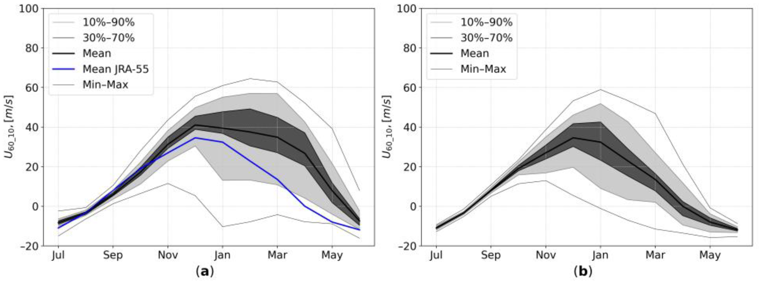
3.1. Model Validation

To assess the reliability of the stratospheric dynamics reconstructions in model experiments using the Isca framework, the main meteorological parameters obtained during the control experiment were compared with the corresponding values in the JRA-55 reanalysis.

The validation of the model showed that the dynamics of the SPV is realistically reproduced. As the effects of the ENSO phases are not symmetric and the observational data account also for such factors as PDO and QBO, there are noticeable differences in the climatological mean values between the control experiment and JRA-55 reanalysis. The monthly mean intensity of the SPV, estimated as the zonal mean zonal wind along the 60° N at the level of 10 hPa (U_{60_10}), in the control experiment, is higher than in the reanalysis data during the whole year (Figure 1a). The maximum differences are observed in the late winter months and in spring. The stronger vortex in model experiment can be explained by neutral boundary conditions without large-scale SST anomalies such as ENSO events that can strongly perturb the vortex and reduce its average intensity [26,27]. In the control experiment, the SPV dynamics reflects the dynamic processes of thermal relaxation in the polar stratosphere. At the same time, Figure 1 shows that, in the control experiment, the variability of the SPV is much higher than in the observational data.

Figure 2 shows the zonal mean structure of the Northern hemisphere atmosphere. In the model data, a colder polar lower stratosphere is observed, while, at the same time, the upper stratosphere (above 30 hPa) is much warmer (Figure 2a,b).

The intensity of the polar night jet is higher in the model data on the heights from the tropopause up to 35 km (Figure 2c,d). In addition, the model does not reproduce the quasi-biennial oscillations (Figure 2e,f) because this requires resolution in the lower stratosphere being no more than 1 km and the sufficiently strong forcing provided by the parameterized nonorographic gravity wave drag [64,65]. Note, however, that it is not our goal, as we aimed to analyze isolated SSTAs’ effect on the stratospheric dynamics, and parameterized gravity wave drag is not included in our Isca configuration.

The analysis of the spatial structure of the vortex shows that SPV at 30 hPa level is centered over the pole and is more intense in the control experiment compared to the reanalysis data (Figure 3).

The shift of the center of the vortex away from the pole partly explains the warmer polar lower stratosphere in the observational data (Figure 3b). This difference in the mean position of the vortex relative to the pole can be explained by the fact that, in the JRA-55 construction, the years with El-Niño and La-Niña events are used, which lead to a shift of the vortex, so the reanalysis data show the deformation of the vortex and its displacement from the pole toward the North Atlantic or Eurasia.

3.2. Intensity of the SPV

First of all, we analyzed the influence of various SST anomalies on the SPV intensity quantified by U_{60_10}. In the “single” experiments with SST anomalies corresponding to the PDO phases (PDO+ and PDO−), there are no statistically significant differences in the SPV intensity with the control experiment data (Figure 4a,c).

The EN experiment shows a weaker vortex than the CTRL experiment (Figure 4a). During the winter months, the average U_{60_10} values in the EN experiment are 40% lower than the control values. For example, in January, U_{60_10} is 39.5 m/s according to the control experiment, which is 15.0 m/s higher than in the experiment with EN anomalies. At the same time, the differences for the CTRL and the EN experiments are statistically significant for the entire extended winter period (November–April) (Figure 4b).

The SPV is weaker both in EN&PDO+ and EN&PDO−, compared to the control experiment. The differences with the CTRL data are statistically significant over the entire extended winter period, except for March in the EN&PDO− data (Figure 4b). Thus, the addition of the positive PDO phase SST anomalies to El Niño anomalies enhances the effect of weakening of the SPV by El Niño (the intensity decreases by 58% in the winter months compared to the control values), while the addition of the negative PDO phase anomalies, on the contrary, weakens this effect (in the EN&PDO− experiment, the vortex is stronger on average by 12% relative to the EN experiment). However, the impact of the negative PDO phase SST anomalies is not stable; for example, for the months of November, December, January, and April, the difference in the intensity of the SPV with the EN experiment is not statistically significant, while, for EN and EN&PDO+, the differences in the SPV intensity are statistically significant throughout the extended winter period except in November.

In the “single” LN experiment, the SPV intensity is lower than in the CTRL experiment, but the anomalies are smaller than in the “single” EN experiment (Figure 4c). The vortex for the winter period (December–February) is weaker than the control values by 19%. At the same time, the differences with the control values are statistically significant for the entire extended winter season (Figure 4d). In contrast to the “merged” experiments with EN, both graphs for the “merged” experiments with LN lie above the “single” LN experiment, i.e., the La Niña effect is weakened by the addition of SST anomalies in the mid-latitudes of the Pacific Ocean. The intensity of the vortex in the LN&PDO+ experiment is statistically indistinguishable from the control values for the winter months (December–March) (Figure 4d). For other “merged” experiments, the effect of the weakening of the SPV is not stable over an extended winter period. Thus, firstly, the response of the SPV to the El Niño and La Niña anomalies is not symmetrical both in terms of the effect (strengthening/weakening of the vortex) and in terms of the intensity. The vortex is weaker in both “single” experiments, but the effect of the El Niño is much more intense than that of the La Niña. The SST anomalies in the mid-latitudes of the Pacific Ocean (PDO+ and PDO−) do not lead to significant changes in the intensity of the SPV in “single” experiments, but, in the “merged” experiments, they significantly correct the effect of SST anomalies in the equatorial zone on the SPV intensity. While the positive phase of the PDO intensifies the effect of the El Niño on the SPV, the negative phase weakens this effect. The SST anomalies corresponding to both phases of the PDO weaken the effect of the La Niña.

This section may be divided by subheadings. It should provide a concise and precise description of the experimental results, their interpretation, and the experimental conclusions that can be drawn.

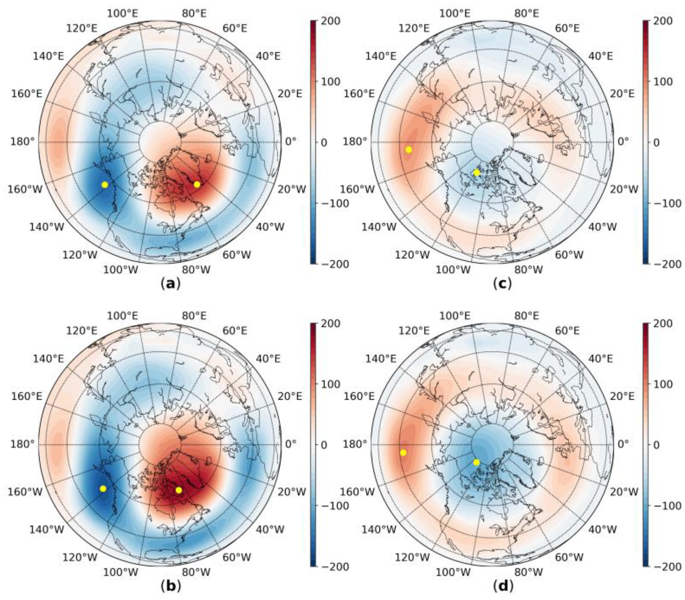
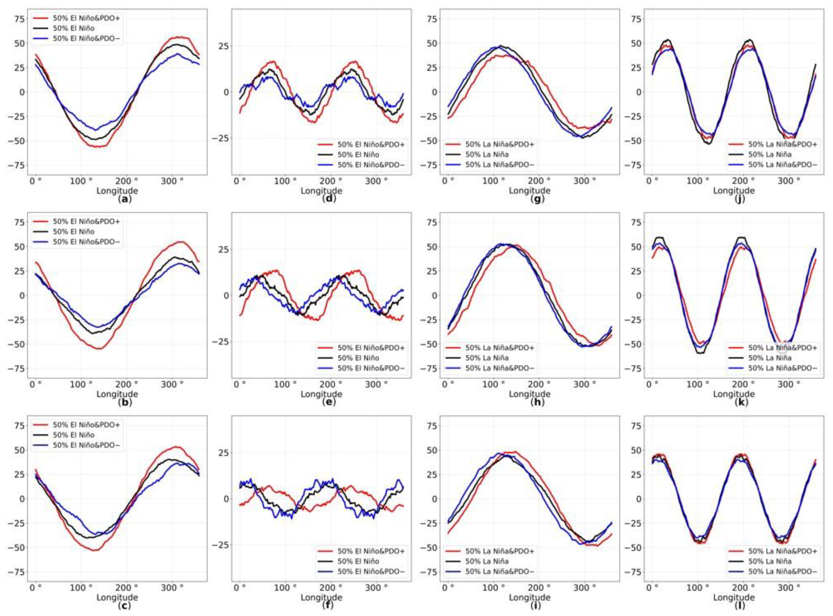
3.3. Planetary Waves Structure

The spatial structure and peculiarities of the quasi-stationary planetary waves’ propagation form the SPV intensity anomalies [66].

The response of the large-scale atmosphere dynamics in the lower and middle troposphere differs significantly in the experiments. Figure 5 shows that with SST anomalies corresponding to the El Niño events, the anomalies of the geopotential heights (hgt) of the surface 500 hPa have the structure of a wave propagating from the tropical zone of the Pacific Ocean to the north-east: with positive anomalies in the central part of the tropics, negative anomalies in the Aleutian Low region, and, again, positive anomalies near the southern tip of Greenland and over the Labrador Sea. This spatial distribution of the hgt anomalies is similar to the Pacific-North American mode, but is slightly shifted to the east. Thus, the strengthening of the Aleutian minimum (the surface of 850 hPa lowers by 100–159 m) and the weakening of the Icelandic minimum (the surface of 850 hPa raises by 100–152 m) are observed (Figure 5a).

In the LN experiments, the response of the pressure field in the lower troposphere is more zonally symmetrical. Figure 5b shows a ring structure of positive hgt anomalies for the surface of 850 hPa, located on average between 40 and 60 N. That is, the distribution of the response resembles the Northern annular mode (NAM). In the polar region, the 850 hPa surface deepens by 50 m on average, while the positive anomalies of the 850 hPa surface in the mid-latitudes of the Northern Hemisphere range from 5 m in the Atlantic Ocean to 90 m in the central Pacific Ocean.

In the “merged” experiments, the pattern of the large-scale pressure field response is the same as in the “single” ones. However, the hgt anomalies are higher by 12% in the region of the Aleutian Low and by 20% in the region of the North Atlantic in the EN&PDO+ experiment compared to anomalies in the EN experiment. In the LN&PDO− experiment, the height anomalies of the surface of 850 hPa in the polar region are 60% higher and their maximum absolute value is 106 m, and, in the mid-latitudes, the anomalies are 11% higher compared to the “single” LN experiment (Figure 5c,d).

As only planetary waves with small wave numbers can penetrate the stratosphere, we analyzed the amplitudes and phases of waves 1 and 2. Figure 6a–f show the amplifications of both waves if the positive phase of the PDO is added to the El Niño (red color), and their weakening if the negative phase is added (in blue). The amplitude of wave 2 increases from December to February in the EN&PDO− experiment (blue color) and decreases in the EN&PDO+ experiment (red color). Wave 2 is fixed in space in the EN&PDO+ experiment and shifts to the west in “single” EN and EN&PDO−.

In contrast to the EN experiments, we do not see much difference between the LN experiments. Only wave 1 shifts to the east in the LN&PDO+.

While comparing experiments with the La Niña boundary condition to the El Niño, we can see that wave 2′s amplitude is much higher (comparable to the amplitude of wave 1) in experiments with the La Niña boundary conditions (Figure 5g–l). Wave 1 in the “single” and “merged” EN and LN experiments are out of phase.

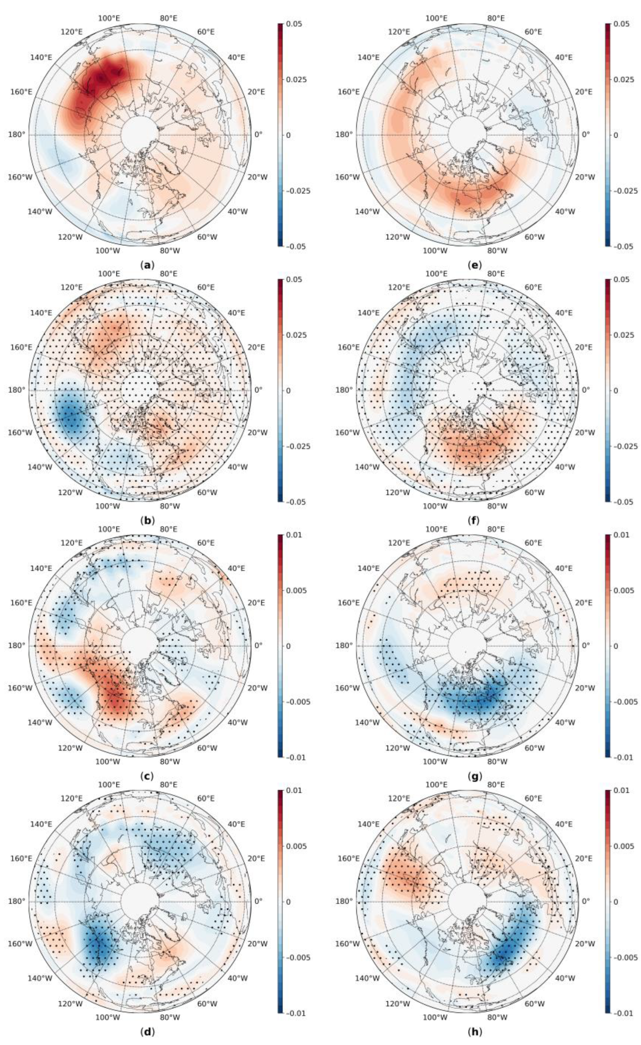
3.4. Planetary Waves Activity

The spatial structure and the intensity of the planetary wave’s propagation were analyzed using Plumb flux analysis. We consider the vertical component of the Plumb flux (Fz) only. In the “single” experiments, the Fz is greater in EN, compared to LN. Moreover, in the EN experiment, the maximum values of the vertical component of the wave activity flux are over eastern Siberia, in LN—over the Labrador Peninsula (Figure 7a,b). Compared to the CTRL experiment, the intensity of the Fz during the El Niño event increases in the region of the eastern Siberia, with the area of the maximum climatological mean Fz values. Whereas during the La Niña events, the vertical flux weakens in this area (Figure 7e,f).

The region of the maximum values of the Fz corresponds to the trough of the planetary wave 1 in the middle troposphere (500 hPa) (Figure S4). During the El Niño events, this is the region of Eastern Siberia and Primorsky Krai (100–120° E, 40–60° N) during the La Niña; it is the area of the Canadian Arctic Archipelago and the Labrador Sea (60–80° W, 50–60° N).

Figure 7c,d shows that the combination of the El Niño and the positive phase of the PDO (EN&PDO+) is characterized by an intensification of the waves’ activity vertical propagation over the western part of Canada and over the Urals, while, in the combination of the El Niño and the negative phase of the PDO (EN&PDO−), the effect is the opposite.

With the SST anomalies formed by the La Niña and the positive PDO phase (LN&PDO+) (Figure 7g), a weakening of the vertical waves’ activity flux is observed over the Canadian Arctic Archipelago and southern Greenland; additionally, in the region of the Urals and Western Siberia, the flow increases compared to the “single” LN. The large-scale SST anomalies corresponding to the La Niña and the negative PDO phase (LN&PDO−) lead to the intensification of the Fz over the western part of the Pacific Ocean in mid-latitudes and to its weakening over the northern North Atlantic, compared to the “single” LN experiment (Figure 7h).

Figure 8 shows the first and second empirical orthogonal functions of the vertical component of the Plumb flux (first and second EOF Fz) at 100 hPa level for the “single” EN and LN experiments. The spatial distribution of the first EOF Fz during the El Niño corresponds to planetary wave 2 and explains up to 23% of the waves’ activity vertical flux variability (Figure 8a), while the second EOF corresponds to wave 1 and explains up to 17% (Figure 8b). In the La Niña events, the situation is the opposite: the first EOF Fz (28%) corresponds to wave 1 (Figure 8c), and the seco EOF Fz (15%) corresponds to wave 2 (Figure 8d).

In order to determine which wave plays the leading role in the formation of the SPV intensity anomalies, the coefficients of determination (R2) between the principal components (PC) of the first and second EOF Fz and the SPV intensity (as U_{60_10}) were calculated.

Table 2. The coefficients of determination (R2) between the principal components of the first and second EOF Fz and U_{60_10} (December–February). Values above 0.15 are bold.

		PC 1	PC 2
CTRL		0.04	0.00
El Niño	N	0.38	0.20
	PDO+	0.10	0.26
	PDO−	0.10	0.18
La Niña	N	0.00	0.20
	PDO+	0.06	0.01
	PDO−	0.18	0.01

shows, that in the CTRL experiment, the roles of the waves cannot be distinguished, and, in the “single” EN experiment, R2 with the PC of the first EOF is 0.38, so it can be concluded that the variability of the intensity of the vertical propagation of wave 2 plays a leading role in the formation of the SPV anomalies. The same can be seen for the La Niña events, where R2 = 0.20 for the second EOF. However, in the “merged” EN&PDO+ and EN&PDO− experiments, the main role goes to the propagation intensity of wave 1, while, at the same time, the coupling is higher in the case of the positive PDO phase. In the “merged” experiments with the La Niña events, a connection between the intensity of the SPV and the PC of the first EOF Fz, which corresponds to wave 2, can be seen only during the negative PDO phase cases.

4. Conclusions

The following results were obtained based on the idealized modeling experiments with different boundary conditions corresponding to the large-scale SST anomalies, such as the ENSO and the PDO:

• It was shown that the large-scale extratropical SST anomalies do not show a statistically significant effect on the dynamics of the stratospheric polar vortex, but they significantly correct the effect of the ENSO modes when added to them. This contradicts the results obtained in [37], which show that the vortex is often weakened during the positive phase of the PDO. However, these works are based on the observational data, in which it is difficult to distinguish the influence of the various factors. It also contradicts the results obtained in the numerical experiments presented in [36].
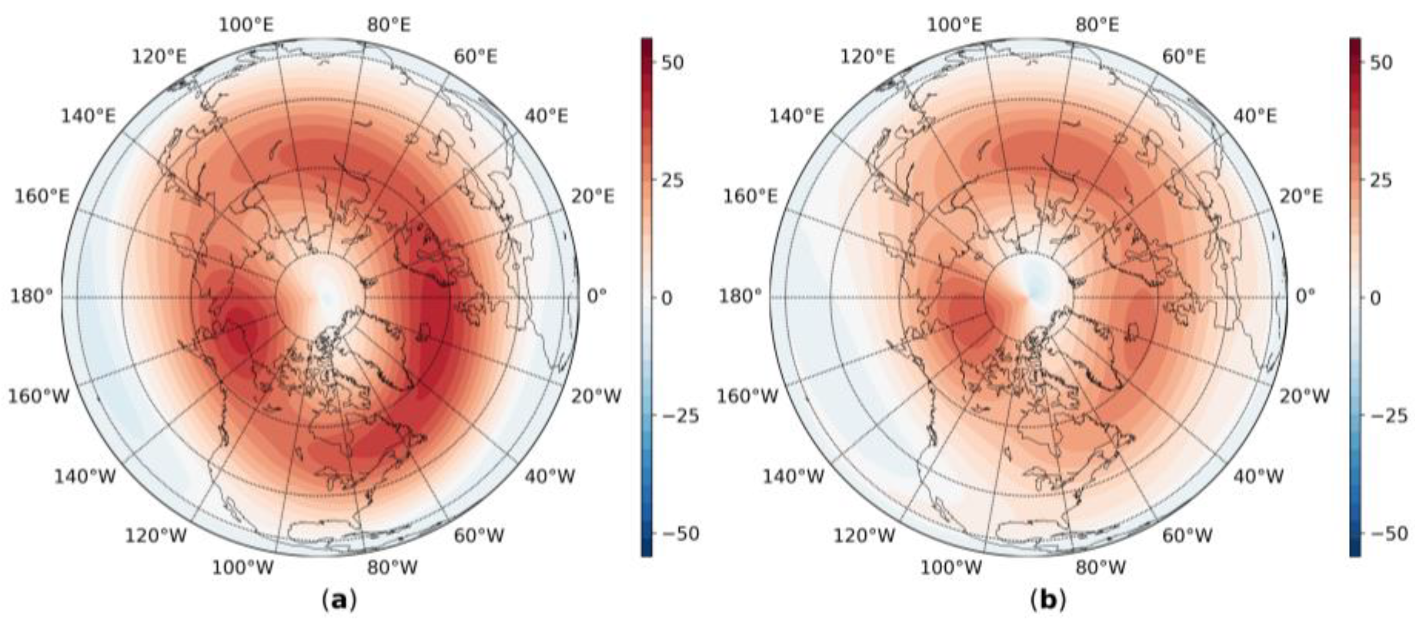
• In the middle troposphere, the El Niño leads to the PNA mode pattern pressure anomalies formation, which is consistent with the previously obtained results ([67,68,69]). At the same time, in our work, we obtained that, when the El Niño occurs during the positive PDO phase, these anomalies increase, and, during the negative phase, the anomalies weaken. The “single” La Niña experiment showed the NAM-pattern pressure anomalies and that they intensify when PDO− added. However, when PDO+ is added, the spatial pattern of the pressure field anomalies is absolutely different and we can find the features of the PNA mode there.
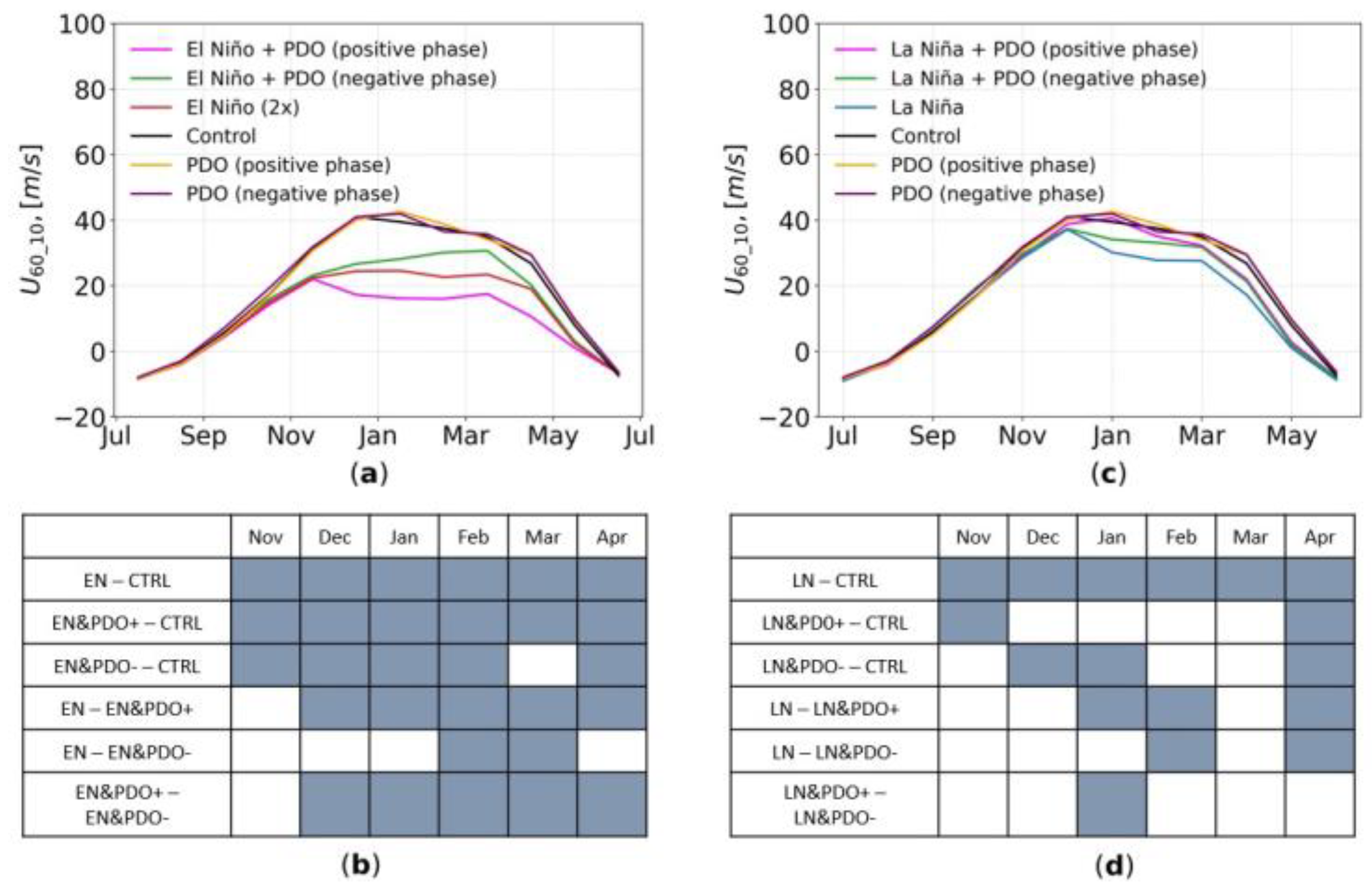
• The intensity of the SPV, expressed as U_{60_10}, is weaker in both EN and LN experiments compared to the CTRL one. The previous papers have shown that, during the La Niña events, the SPV is stronger than the climatic mean [30]. This is explained by the fact that the average intensity of the vortex is lower according to the reanalysis data, compared to the CTRL experiment, since, in averaging over the observational data, weakened SPV states during the El Niño events are used. However, we showed that the effect of the El Niño and La Niña events on the SPV intensity is asymmetrical, so that, in the “single” EN experiment, the vortex is weaker by 40% than in the CTRL, and, in the “single” LN, the decrease is on average 19%. However, this characteristic is sensitive both to the intensity of the polar night jet and to the position of the SPV relative to the pole. Therefore, an additional analysis of the change in the spatial structure of the vortex and its centering over to the pole is required. Additionally, it is important to remember that, in the SST, the anomalies in this study’s experiments conducted were doubled and, in reality, the response of the stratosphere dynamics could be weaker.
• We showed that asymmetry is seen in the PDO mode’s influence on the effect of the ENSO on stratosphere dynamics. During the positive phase of the PDO, the impact of the El Niño events increases. When the negative PDO phase is added, the El Niño effect weakens: the vortex is stronger than in the “single” EN experiments, but is weaker than in the control experiment. The La Niña effect weakens during both positive and negative PDO phases.
• The formation of the SPV intensity anomalies during the El Niño events in “single” experiments occurs mainly due to planetary wave 2 variability, which explains up to 38% of the SPV intensity variability. In the case of the “merged” experiments, in EN&PDO+, wave 1 adopts the leading role in the formation of the SPV intensity anomalies, which explains up to 26% of the SPV intensity variability.
• In the “single” LN experiments, the formation of the SPV intensity anomalies occurs mainly due to wave 1 variability, which explains up to 20% of its variability. However, only in the LN&PDO− experiments can a connection between wave 2 and the SPV intensity be seen (18%).
• Our analysis showed that the dynamical response of the stratosphere-troposphere interaction is very sensitive to the meridional gradient of the SST anomalies between the tropical zone and mid-latitudes. The PDO mode can significantly correct the ENSO effect. The El Niño and positive PDO phase lead to the strongest meridional SST gradient between the tropical zone and the mid-latitudes and the strongest effect on the vortex. On the contrary, the El Niño and negative PDO phase lead to the weakest gradient and a weakening effect on the vortex.

This study is based on the idealized modeling using doubled SST anomalies corresponding to the ENSO (Niño-3 region) and the PDO modes. The SST anomalies in other areas of the World Ocean and processes such as QBO, Maden-Julian oscillations, etc., also influence the dynamics of the quasi-stationary planetary waves. Additionally, these effects can non-linearly interact with the effect of the ENSO and the PDO. The question of the linearity of the response to the amplitude of the ENSO and the PDO anomalies also remains open. Therefore, further study of these processes is needed.

References

1. Smith, K.L.; Kushner, P.J. Linear interference and the initiation of extratropical stratosphere-troposphere interactions. J. Geophys. Res. 2012, 117, D13107. [Google Scholar] [CrossRef] [Green Version]
2. Kidston, J.; Scaife, A.A.; Hardiman, S.C.; Mitchell, D.M.; Butchart, N.; Baldwin, M.P.; Gray, L.J. Stratospheric influence on tropospheric jet streams, storm tracks and surface weather. Nat. Geosci. 2015, 8, 433–440. [Google Scholar] [CrossRef]
3. Scaife, A.A.; Comer, R.E.; Dunstone, N.J.; Knight, J.R.; Smith, D.M.; MacLachlan, C.; Martin, N.; Peterson, K.A.; Rowlands, D.; Carroll, E.B.; et al. Tropical rainfall, Rossby waves and regional winter climate predictions. Q. J. R. Meteorol. Soc. 2016, 143, 1–11. [Google Scholar] [CrossRef]
4. Nie, Y.; Scaife, A.A.; Ren, H.L.; Comer, R.E.; Andrews, M.B.; Davis, P.; Martin, N. Stratospheric initial conditions provide seasonal predictability of the North Atlantic and Arctic Oscillations. Environ. Res. Lett. 2019, 14, 034006. [Google Scholar] [CrossRef]
5. Xiong, X.; Liu, X.; Wu, W.; Knowland, K.E.; Yang, F.; Yang, Q.; Zhou, D.K. Impact of Stratosphere on Cold Air Outbreak: Observed Evidence by CrIS on SNPP and Its Comparison with Models. Atmosphere 2022, 13, 876. [Google Scholar] [CrossRef]
6. Vitart, F.; Brown, A. S2S Forecasting: Towards Seamless Prediction. WMO Bull. 2019, 68, 70–74. [Google Scholar]
7. Vitart, F.; Robertson, A.W. The sub-seasonal to seasonal prediction project (S2S) and the prediction of extreme events. NPJ Clim. Atmos. 2018, 1, 3. [Google Scholar] [CrossRef] [Green Version]
8. Baldwin, M.P.; Dunkerton, T.J. Stratospheric harbingers of anomalous weather regimes. Science 2001, 294, 581–584. [Google Scholar] [CrossRef] [PubMed]
9. Thompson, D.W.; Wallace, J.M. Regional climate impacts of the Northern Hemisphere annular mode. Science 2001, 293, 85–89. [Google Scholar] [CrossRef] [PubMed] [Green Version]
10. Wallace, J.M.; Thompson, D.W. Annular modes and climate prediction. Phys. Today 2002, 55, 28–34. [Google Scholar] [CrossRef] [Green Version]
11. Baldwin, M.P.; Stephenson, D.B.; Thompson, D.W.; Dunkerton, T.J.; Charlton, A.J.; O’Neill, A. Stratospheric memory and skill of extended-range weather forecasts. Science 2003, 301, 636–640. [Google Scholar] [CrossRef]
12. Kolstad, E.W.; Breiteig, T.; Scaife, A.A. The association between stratospheric weak polar vortex events and cold air outbreaks in the Northern Hemisphere. Q. J. R. Meteorol. Soc. 2010, 136, 886–893. [Google Scholar] [CrossRef] [Green Version]
13. Gerber, E.P.; Butler, A.; Calvo, N.; Charlton-Perez, A.; Giorgetta, M.; Manzini, E.; Perlwitz, J.; Polvani, L.M.; Sassi, F.; Scaife, A.A.; et al. Assessing and understanding the impact of stratospheric dynamics and variability on the Earth system. Bull. Am. Meteorol. Soc. 2012, 93, 845–859. [Google Scholar] [CrossRef] [Green Version]
14. Tomassini, L.; Gerber, E.P.; Baldwin, M.P.; Bunzel, F.; Giorgetta, M. The role of stratosphere-troposphere coupling in the occurrence of extreme winter cold spells over northern Europe. J. Adv. Model. Earth Syst. 2012, 4. [Google Scholar] [CrossRef]
15. Hitchcock, P.; Simpson, I.R. The downward influence of stratospheric sudden warmings. J. Atmos. Sci. 2014, 71, 3856–3876. [Google Scholar] [CrossRef]
16. Nakamura, T.; Yamazaki, K.; Iwamoto, K.; Honda, M.; Miyoshi, Y.; Ogawa, Y.; Tomikawa, Y.; Ukita, J. The stratospheric pathway for Arctic impacts on midlatitude climate. Geophys. Res. Lett. 2016, 43, 3494–3501. [Google Scholar] [CrossRef] [Green Version]
17. Charlton-Perez, A.J.; Ferranti, L.; Lee, R.W. The influence of the stratospheric state on North Atlantic weather regimes. Q. J. R. Meteorol. Soc. 2018, 144, 1140–1151. [Google Scholar] [CrossRef] [Green Version]
18. Kretschmer, M.; Coumou, D.; Agel, L.; Barlow, M.; Tziperman, E.; Cohen, J. More-persistent weak stratospheric polar vortex states linked to cold extremes. Bull. Am. Meteorol. Soc. 2018, 99, 49–60. [Google Scholar] [CrossRef]
19. Kretschmer, M.; Cohen, J.; Matthias, V.; Runge, J.; Coumou, D. The different stratospheric influence on cold-extremes in Eurasia and North America. NPJ Clim. Atmos. 2018, 1, 44. [Google Scholar] [CrossRef] [Green Version]
20. Gerber, E.P.; Orbe, C.; Polvani, L.M. Stratospheric influence on the tropospheric circulation revealed by idealized ensemble forecasts. Geophys. Res. Lett. 2009, 36, L24801. [Google Scholar] [CrossRef] [Green Version]
21. Karpechko, A.Y. Predictability of sudden stratospheric warmings in the ECMWF Extended-Range Forecast System. Mon. Weather Rev. 2018, 146, 1063–1075. [Google Scholar] [CrossRef]
22. Tripathi, O.P.; Baldwin, M.; Charlton-Perez, A.; Charron, M.; Eckermann, S.D.; Gerber, E.; Harrison, R.G.; Jackson, D.R.; Kim, B.M.; Kuroda, Y.; et al. The predictability of the extratropical stratosphere on monthly time-scales and its impact on the skill of tropospheric forecasts. Q. J. R. Meteorol. Soc. 2015, 141, 987–1003. [Google Scholar] [CrossRef]
23. Scaife, A.A.; Karpechko, A.Y.; Baldwin, M.P.; Brookshaw, A.; Butler, A.; Eade, R.; Gordon, M.E.; MacLachlan, C.; Martin, N.A.; Dunstone, N.; et al. Seasonal winter forecasts and the stratosphere. Atmos. Sci. Lett. 2016, 17, 51–56. [Google Scholar] [CrossRef] [Green Version]
24. Volodin, E.M. Natural climate oscillations on decadal time scales. Fund. Appl. Climatol. 2015, 1, 78–95. [Google Scholar]
25. Kim, H.M.; Webster, P.J.; Curry, J.A. Evaluation of short-term climate change prediction in multi-model CMIP5 decadal hindcasts. Geophys. Res. Lett. 2012, 39. [Google Scholar] [CrossRef]
26. Calvo, N.; García-Herrera, R.; Garcia, R.R. The ENSO signal in the stratosphere. Ann. N. Y. Acad. Sci. 2008, 1146, 16–31. [Google Scholar] [CrossRef] [Green Version]
27. Manzini, E. ENSO and the stratosphere. Nat. Geosci. 2009, 2, 749–750. [Google Scholar] [CrossRef]
28. Mo, K.C.; Livezey, R.E. Tropical-extratropical geopotential height teleconnections during the Northern Hemisphere winter. Mon. Weather Rev. 1986, 114, 2488–2515. [Google Scholar] [CrossRef]
29. Manzini, E.; Giorgetta, M.A.; Esch, M.; Kornblueh, L.; Roeckner, E. The influence of sea surface temperatures on the northern winter stratosphere: Ensemble simulations with the MAECHAM5 model. J. Clim. 2006, 19, 3863–3881. [Google Scholar] [CrossRef] [Green Version]
30. Rao, J.; Ren, R. Asymmetry and nonlinearity of the influence of ENSO on the northern winter stratosphere: 1. Observations. J. Geophys. Res. Atmos. 2016, 121, 9000–9016. [Google Scholar] [CrossRef] [Green Version]
31. Ashok, K.; Behera, S.; Rao, A.S.; Weng, H.; Yamagata, T. El Niño Modoki and its teleconnection. J. Geophys. Res. 2007, 112, C11007. [Google Scholar] [CrossRef]
32. Xie, F.; Li, J.; Tian, W.; Feng, J.; Huo, Y. Signals of El Niño Modoki in the tropical tropopause layer and stratosphere. Atmos. Chem. Phys. 2012, 12, 5259–5273. [Google Scholar] [CrossRef] [Green Version]
33. Garfinkel, C.I.; Hartmann, D.L. Different ENSO teleconnections and their effects on the stratospheric polar vortex. J. Geophys. Res. Atmos. 2008, 113, D18. [Google Scholar] [CrossRef] [Green Version]
34. Kushnir, Y.; Robinson, W.A.; Bladé, I.; Hall, N.M.J.; Peng, S.; Sutton, R. Atmospheric GCM response to extratropical SST anomalies: Synthesis and evaluation. J. Clim. 2002, 15, 2233–2256. [Google Scholar] [CrossRef]
35. Jadin, E.A.; Wei, K.; Zyulyaeva, Y.A.; Chen, W.; Wang, L. Stratospheric wave activity and the Pacific Decadal Oscillation. J. Atmos. Sol.-Terr. Phys. 2010, 72, 1163–1170. [Google Scholar] [CrossRef]
36. Hurwitz, M.M.; Newman, P.A.; Garfinkel, C.I. On the influence of North Pacific sea surface temperature on the Arctic winter climate. J. Geophys. Res. Atmos. 2012, 117, D19. [Google Scholar] [CrossRef]
37. Woo, S.H.; Sung, M.K.; Son, S.W.; Kug, J.S. Connection between weak stratospheric vortex events and the Pacific Decadal Oscillation. Clim. Dyn. 2015, 45, 3481–3492. [Google Scholar] [CrossRef]
38. Kren, A.C.; Marsh, D.R.; Smith, A.K.; Pilewskie, P. Wintertime Northern Hemisphere response in the stratosphere to the Pacific decadal oscillation using the Whole Atmosphere Community Climate Model. J. Clim. 2016, 29, 1031–1049. [Google Scholar] [CrossRef]
39. Wang, W.; Matthes, K.; Omrani, N.E.; Latif, M. Decadal variability of tropical tropopause temperature and its relationship to the Pacific Decadal Oscillation. Sci. Rep. 2016, 6, 29537. [Google Scholar] [CrossRef] [Green Version]
40. Zyulyaeva, Y.A.; Zhadin, E.A. Analysis of three-dimensional Eliassen-Palm fluxes in the lower stratosphere. Russ. Meteorol. Hydrol. 2009, 34, 483. [Google Scholar] [CrossRef]
41. Brierley, C.M.; Fedorov, A.V. Relative importance of meridional and zonal sea surface temperature gradients for the onset of the ice ages and Pliocene-Pleistocene climate evolution. Paleoceanography 2010, 25. [Google Scholar] [CrossRef] [Green Version]
42. Rind, D.; Suozzo, R.; Balachandran, N.K.; Prather, M.J. Climate change and the middle atmosphere. Part I: The doubled CO2 climate. J. Atmos. Sci. 1990, 47, 475–494. [Google Scholar] [CrossRef]
43. Olsen, M.A.; Schoeberl, M.R.; Nielsen, J.E. Response of stratospheric circulation and stratosphere-troposphere exchange to changing sea surface temperatures. J. Geophys. Res. Atmos. 2007, 112, D16. [Google Scholar] [CrossRef] [Green Version]
44. Rao, J.; Ren, R.; Xia, X.; Shi, C.; Guo, D. Combined impact of El Niño–Southern Oscillation and Pacific Decadal Oscillation on the northern winter stratosphere. Atmosphere 2019, 10, 211. [Google Scholar] [CrossRef] [Green Version]
45. Bond, N.A.; Overland, J.E.; Spillane, M.; Stabeno, P. Recent shifts in the state of the North Pacific. Geophys. Res. Lett. 2003, 30. [Google Scholar] [CrossRef] [Green Version]
46. Di Lorenzo, E.; Schneider, N.; Cobb, K.M.; Franks, P.J.S.; Chhak, K.; Miller, A.J.; McWilliams, J.C.; Bograd, S.J.; Arango, H.; Curchitser, E.; et al. North Pacific Gyre Oscillation links ocean climate and ecosystem change. Geophys. Res. Lett. 2008, 35. [Google Scholar] [CrossRef] [Green Version]
47. Hurrell, J.W.; Hack, J.J.; Shea, D.; Caron, J.M.; Rosinski, J. A new sea surface temperature and sea ice boundary dataset for the Community Atmosphere Model. J. Clim. 2008, 21, 5145–5153. [Google Scholar] [CrossRef]
48. Rayner, N.A.; Parker, D.E.; Horton, E.B.; Folland, C.K.; Alexander, L.V.; Rowell, D.P.; Kent, E.C.; Kaplan, A. Global analyses of sea surface temperature, sea ice, and night marine air temperature since the late nineteenth century. J. Geophys. Res. Atmos. 2003, 108, D14. [Google Scholar] [CrossRef] [Green Version]
49. Reynolds, R.W.; Smith, T.M.; Liu, C.; Chelton, D.B.; Casey, K.S.; Schlax, M.G. Daily high-resolution-blended analyses for sea surface temperature. J. Clim. 2007, 20, 5473–5496. [Google Scholar] [CrossRef]
50. Taylor, K.E.; Williamson, D.; Zwiers, F. The Sea Surface Temperature and Sea-Ice Concentration Boundary Conditions for AMIP II Simulations; Lawrence Livermore National Laboratory: Livermore, CA, USA, 2000; Volume 28.
51. Kobayashi, S.; Ota, Y.; Harada, Y.; Ebita, A.; Moriya, M.; Onoda, H.; Onogi, K.; Kamahori, H.; Kobayashi, C.; Endo, H.; et al. The JRA-55 reanalysis: General specifications and basic characteristics. J. Meteorol. Soc. 2015, 93, 5–48. [Google Scholar] [CrossRef] [Green Version]
52. Vallis, G.K.; Colyer, G.; Geen, R.; Gerber, E.; Jucker, M.; Maher, P.; Paterson, A.; Pietschnig, M.; Penn, J.; Thomson, S.I. Isca, v1. 0: A framework for the global modelling of the atmospheres of Earth and other planets at varying levels of complexity. Geosci. Model Dev. 2018, 11, 843–859. [Google Scholar] [CrossRef] [Green Version]
53. Dee, D.P.; Uppala, S.M.; Simmons, A.J.; Berrisford, P.; Poli, P.; Kobayashi, S.; Andrae, U.; Balmaseda, M.A.; Balsamo, G.; Bauer, P.; et al. The ERA-Interim reanalysis: Configuration and performance of the data assimilation system. Q. J. R. Meteorol. Soc. 2011, 137, 553–597. [Google Scholar] [CrossRef]
54. Thomson, S.I.; Vallis, G.K. Atmospheric response to SST anomalies. Part I: Background-state dependence, teleconnections, and local effects in winter. J. Atmos. Sci. 2018, 75, 4107–4124. [Google Scholar] [CrossRef]
55. Fortuin, J.P.; Langematz, U. Update on the global ozone climatology and on concurrent ozone and temperature trends. Proc. SPIE 1995, 2311, 207–216. [Google Scholar]
56. Jucker, M.; Gerber, E.P. Untangling the annual cycle of the tropical tropopause layer with an idealized moist model. J. Clim. 2017, 30, 7339–7358. [Google Scholar] [CrossRef]
57. Trenberth, K.E. The definition of El Niño. Bull. Am. Meteorol. Soc. 1997, 78, 2771–2778. [Google Scholar] [CrossRef]
58. Kug, J.S.; Jin, F.F.; An, S.I. Two types of El Niño events: Cold tongue El Niño and warm pool El Niño. J. Clim. 2009, 22, 1499–1515. [Google Scholar] [CrossRef]
59. Tseng, J.C.-H. An ISOMAP Analysis of Sea Surface Temperature for the Classification and Detection of El Niño & La Niña Events. Atmosphere 2022, 13, 919. [Google Scholar]
60. Meehl, G.A.; Teng, H. Multi-model changes in El Niño teleconnections over North America in a future warmer climate. Clim. Dyn. 2007, 29, 779–790. [Google Scholar] [CrossRef]
61. Hare, S.R. Low Frequency Climate Variability and Salmon Production. Ph.D. Dissertation, University of Washington, Seattle, WA, USA, 1996. [Google Scholar]
62. Zhang, Y. An Observational Study of Atmosphere-Ocean Interactions in the Northern Oceans on Interannual and Interdecadal Time-Scales. Ph.D. Dissertation, University of Washington, Seattle, WA, USA, 1996. [Google Scholar]
63. Plumb, R.A. On the three-dimensional propagation of stationary waves. J. Atmos. Sci. 1985, 42, 217–229. [Google Scholar] [CrossRef]
64. Anstey, J.A.; Scinocca, J.F.; Keller, M. Simulating the QBO in an atmospheric general circulation model: Sensitivity to resolved and parameterized forcing. J. Atmos. Sci. 2016, 73, 1649–1665. [Google Scholar] [CrossRef]
65. Lott, F.; Rani, R.; Podglajen, A.; Codron, F.; Guez, L.; Hertzog, A.; Plougonven, R. Direct comparison between a non orographic gravity wave drag scheme and constant level balloons. J. Geophys. Res. Atmos. 2022; in press. [Google Scholar]
66. Matsuno, T. A dynamical model of the stratospheric sudden warming. J. Atmos. Sci. 1971, 28, 1479–1494. [Google Scholar] [CrossRef]
67. Gushchina, D.; Kolennikova, M.; Dewitte, B.; Yeh, S.W. On the relationship between ENSO diversity and the ENSO atmospheric teleconnection to high-latitudes. Int. J. Climatol. 2022, 42, 1303–1325. [Google Scholar] [CrossRef]
68. Zhu, Z.; Li, T. A new paradigm for continental U.S. summer rainfall variability: Asia–North America teleconnection. J. Clim. 2016, 29, 7313–7327. [Google Scholar] [CrossRef]
69. Zhu, Z.; Li, T. Amplified contiguous United States summer rainfall variability induced by East Asian monsoon intedecadal change. Clim. Dyn. 2018, 50, 3523–3536. [Google Scholar] [CrossRef]
Figure 1. Long-term averaged monthly mean values of the intensity of the stratospheric polar vortex (SPV), zonal mean zonal wind along 60° N at 10 hPa [m/s] and its 10th, 30th, 70th, and 90th percentiles, according to the control experiment (a) and JRA-55 reanalysis data (b). The data for the control experiment are provided for 100 years, and the JRA-55 reanalysis data for the period [1958/59–2020/21].
Atmosphere 14 00459 g001
Figure 2. Winter (December–February) zonal mean temperature [K], (a), zonal wind [m/s], (c) and standard deviation of the zonal wind [m/s] (e) according to the control experiment and their difference with the winter (December–February) zonal mean temperature [K], (b), zonal wind [m/s], and (d) standard deviation of the zonal wind [m/s] (f) according to the reanalysis data JRA-55. The average values of the control experiment were calculated for 100 years, and for the JRA-55 reanalysis averaged period is [1958/59–2020/21]. Statistically significant differences at the 1% level (b,d) are marked with dots.
Atmosphere 14 00459 g002
Figure 3. Long-term averaged spatial structure of the zonal wind [m/s] for the winter period (December–February) at the level of 30 hPa according to the control experiment (averaging period 100 years) (a), according to the JRA-55 reanalysis data (averaging period [1958/59–2020/21]) (b).
Atmosphere 14 00459 g003
Figure 4. Monthly mean values of the SPV intensity, [m/s], averaged over 100 years according to the numerical experiments data: (a) CTRL (in black), EN (in red), PDO+ (yellow), PDO− (violet), EN&PDO+ (pink), and EN&PDO− (green); (c) CTRL (in black), LN (blue), PDO+ (yellow), PDO− (violet), LN&PDO+ (pink), and LN&PDO− (green). (b,d) are tables of statistically significant differences between the intensity of the SPV obtained in different experiments, the months with statistically significant differences at 5% level are marked in dark gray.
Atmosphere 14 00459 g004
Figure 5. Differences of winter (December–February) geopotential heights for the surface 850 hPa between (a) EN and the CTRL experiments, (b) LN and the CTRL experiments, (c) EN&PDO+ and the CTRL experiment, and (d) LN&PDO− and the CTRL experiment, [m]. The position of the maximum absolute values of the hgt anomalies are marked by yellow dots.
Atmosphere 14 00459 g005
Figure 6. The 50th percentile of the phases and amplitudes of wave 1 in December (a), January (b), and February (c) and wave 2 in December (d), January (e), and February (f) along 60° N at 500 hPa in the EN experiment (black), EN&PDO+ (red), and EN&PDO− (blue) calculated over 99 model years. The 50th percentile of the phases and amplitudes of wave 1 in December (g), January (h), and February (i) and wave 2 in December (j), January (k), and February (l) along 60° N at 500 hPa in the experiments LN (black), LN&PDO+ (red), and LN&PDO− (blue) calculated over 99 model years.
Atmosphere 14 00459 g006
Figure 7. The vertical component of the Plumb flux (Fz) at the 100 hPa level in EN (a) and LN (e) experiments, and their differences from the Fz in the CTRL experiment (b,f), respectively. Statistically significant differences of the mean values at the 5% level (b,f) are marked with dots. The differences between the Fz in the EN&PDO+ (c), EN&PDO− (d), LN&PDO+ (g), and LN&PDO− (h) and the corresponding “single” ENSO experiments.
Atmosphere 14 00459 g007
Figure 8. The spatial structure of the first (a,c) and second (b,d) empirical orthogonal functions of the vertical component of the Plumb flux (first and second EOF Fz) obtained from the EN (a,b) and LN (c,d) experiments at the 100 hPa level.
Atmosphere 14 00459 g008