Article

Telluric Currents Generated by Solar Flare Radiation: Physical Model and Numerical Estimations

1
Pushkov Institute of Terrestrial Magnetism, Ionosphere, and Radio Wave Propagation, Russian Academy of Sciences, 108840 Moscow, Russia
2
Joint Institute for High Temperatures, Russian Academy of Sciences, 125412 Moscow, Russia
*
Author to whom correspondence should be addressed.
Atmosphere 2023, 14(3), 458; https://doi.org/10.3390/atmos14030458
Submission received: 30 November 2022 / Revised: 31 January 2023 / Accepted: 8 February 2023 / Published: 24 February 2023
(This article belongs to the Special Issue The Influence of Solar and Astronomical Factors on Earth)

Abstract

:
The current studies of solar-terrestrial relations and possible impact of space weather on the seismic activity are based on statistical analysis without detailed consideration of possible physical mechanism that results in fuzzy and contradictory conclusions. We propose to consider a hypothesis of electromagnetic earthquake triggering by a sharp rise of telluric currents in lithosphere including crust faults due to interaction of solar flare X-ray radiation with ionosphere-atmosphere-lithosphere system resulted in a rise of telluric currents in the crust faults. This hypothesis is based on field and laboratory experiments carried out in Russia within the last forty years and clearly demonstrated a possibility of earthquake triggering by electric current injected into the fault. We developed a mathematical model and computer code for numerical estimations of telluric currents generated by solar flare radiations. The obtained numerical results demonstrate that solar flares can cause variations in the density of telluric currents in the crust faults, comparable to the current densities generated in the Earth’s crust by artificial pulsed power sources capable to trigger earthquakes. Consequently, the triggering of seismic events is possible not only by artificial sources of electric current, but also by ionospheric disturbances caused by strong solar flares.

1. Introduction

It is well known that earthquakes can be triggered by external actions such as passing the seismic waves from distant strong earthquakes [1], variation of pore pressure in rocks [2], lunar-solar tides [3], etc., when the earthquake source is located in the crust fault close to the critical stress-strain state [4]. It is natural to suppose that the Sun similarly may provoke earthquakes during strong solar flares resulted in variations of solar wind density and followed by strong geomagnetic storms [5]. Since Aristotle’s observations [6] that earthquakes occur more frequently at the night than during the day, the search for solar-terrestrial relations resulted in earthquake triggering has continued [7,8,9,10,11,12,13,14,15,16,17,18,19,20,21,22,23,24,25,26]. There are some attempts to relate the seismic activity with the sunspot number [7,8,9,10,11,12], geomagnetic storms [13,14,15,16], diurnal Sq-variations [17,18], geomagnetic jerks [19,20], solar wind [21], high-energy particles flow density [22,23], and solar flares [24,25,26]. The results obtained to date are fuzzy, as indicated in [27], and in some cases – contradictive (e.g., in [13,14], a positive correlation between solar and seismic activities was found, and in [21], a negative correlation was demonstrated). Moreover, in [27,28], it is stated that no statistically significant correlation of the global seismicity with one of the possible mechanisms indicated above has been demonstrated yet. It should be noted that all studies ([7,8,9,10,11,12,13,14,15,16,17,18,19,20,21,22,23,24,25,26,27,28], and references therein) are statistical only. They tested statistically only simple hypothesis of possible correlation or an absence of correlation of solar activity and Earth’s seismicity. No physical mechanisms of solar-terrestrial relations resulted in the earthquake triggering were considered in details, and only phenomenological approach was employed. This simplified analysis of the solar-terrestrial relation may provide false results and wrong conclusions.
For a detailed analysis of solar-terrestrial relations that can affect seismic activity, it seems appropriate to consider the hypothesis of the possible earthquake triggering by electromagnetic action of a solar flare radiation on the earthquake preparation area proposed in [25]. This hypothesis is well substantiated by real field observations and laboratory experiments on the study of a new triggering phenomenon in seismology, namely, electromagnetic earthquake triggering due to interaction of electric and electromagnetic fields with rocks and faults in the Earth’s crust under critical stress-strain conditions [29].
For numerical estimations of telluric currents generated in the Earth crust by solar flare radiations and for analysis of their earthquake triggering potential we developed a mathematical model and computer code. The code provides a possibility of numerical simulation of electromagnetic impact of various space weather phenomena on the lithosphere resulted in earthquake triggering.

2. Electric Field Generated by the Perturbation of Ionospheric Conductivity

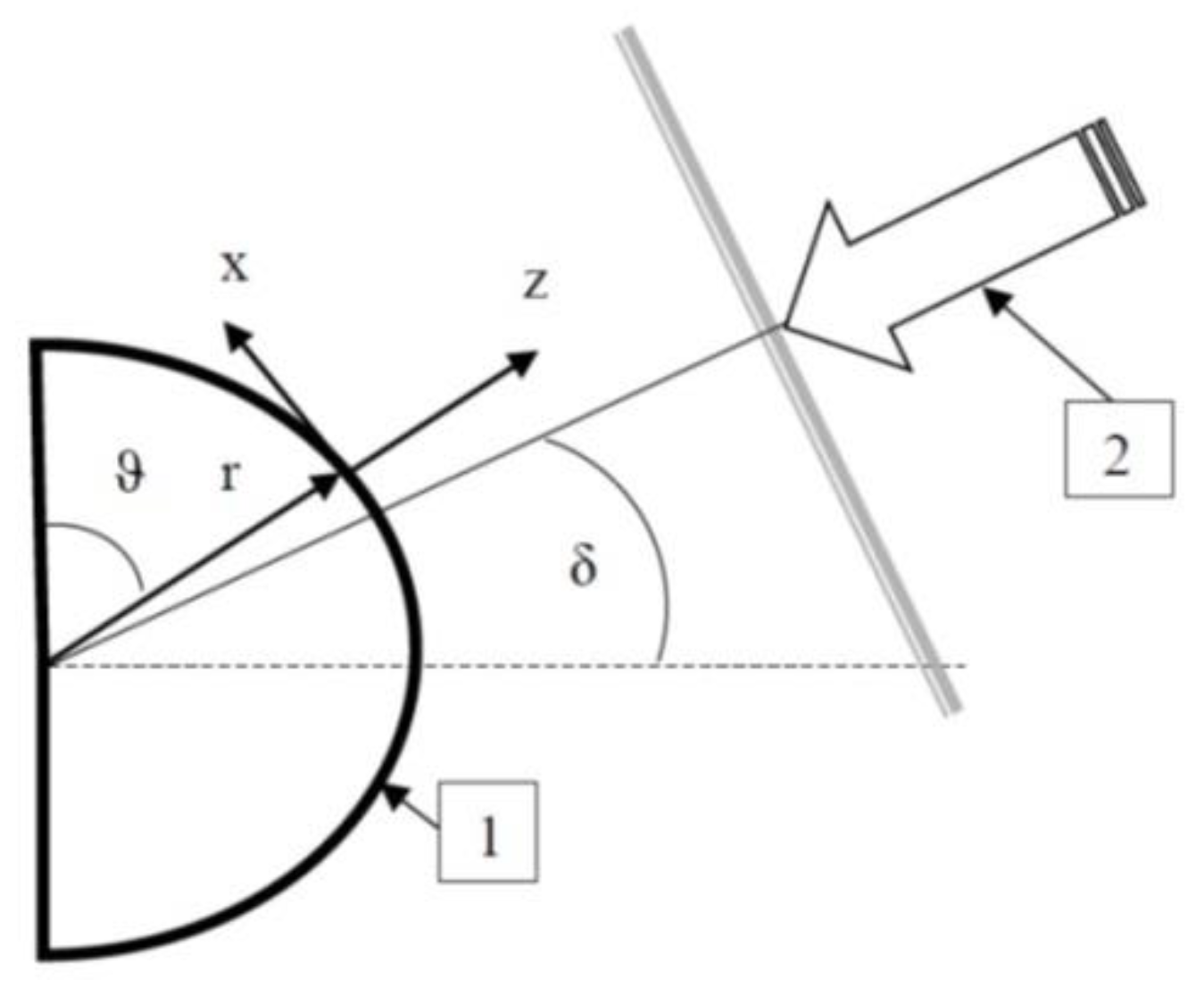
We assume that a flat flux of ionizing radiation from a solar flare falls on a spherical ionosphere, as shown in Figure 1, and introduce a spherical coordinate system (r, θ, φ), where r is the distance from the center of the Earth, ψ is the latitude, φ is the longitude, ϑ = π/2—ψ is the colatitude.
The electric field Eext in the ionosphere is directed parallel to the Earth surface. The absorption of solar flare radiation in the ionosphere results in its additional ionization and conductivity variations. The variation of ionosphere conductivity in an external electric field is accompanied by the occurrence of an additional electric current in the ionosphere and, accordingly, an electric field. The magnetic field induction B and the electric field E comply with Maxwell equation:
× E = B t   ;   × B = μ 0 [ σ ^ ( r , t ) E + j e x t ( r ) ]
where μ0 is the magnetic constant, σ ^ ( r , t ) is the conductivity tensor of the ionospheric plasma, jext is the external electric current that creates in the ionosphere with undisturbed conductivity σ ^ ( r ) an external constant electric and magnetic fields (Eext, Bext) satisfying stationary Maxwell equations:
× E e x t = 0   ;   × B e x t = μ 0 [ σ ^ ( r ) E e x t + j e x t ( r ) ]
Subtracting Equation (2) from Equation (1), we obtain a system of equations for perturbations of electric field e = EEext and magnetic field b = BBext in the following form:
× e = b t   ;   × b = μ 0 σ ^ ( r , t ) e + μ 0 [ σ ^ ( r , t ) σ ^ ( r ) ] E e x t
From the system of Equation (3) we derive the equation for the perturbation of the electric field:
× ( × e ) + μ 0 t σ ^ ( r , t ) e = μ 0 t σ ^ ( r , t ) E e x t
The horizontal size of the region of conductivity perturbed by a solar flare is of the order of the Earth radius Re, and the vertical size is of the order of the thickness of conductive layer of the ionosphere. Thus, in Equation (4), we may neglect the horizontal derivatives, that corresponds to the fact that during the characteristic period of the field change the ionospheric currents and fields diffuse in the horizontal direction to a distance much less than the horizontal size. We introduce a local Cartesian coordinate system with z-axis (z = rRe, |z| << Re) directed vertically upwards, x-axis directed to the equator, and y-axis directed to the east in the northern hemisphere. The lower boundary of the ionosphere is located in the plane z = z1, and the Earth surface is located in the plane z = 0. In this coordinate system, the ionospheric conductivity tensor has the following view [30]:
σ ^ = ( σ c o s 2 I + σ P s i n 2 I σ H s i n I ( σ σ P ) s i n I c o s I σ H s i n I σ P σ H c o s I ( σ σ P ) s i n I c o s I σ H c o s I σ s i n 2 I + σ P c o s 2 I )
where σ is the longitudinal conductivity along the geomagnetic field, σP, σH are the Pedersen and Hall conductivities of the ionospheric plasma, I is the geomagnetic field inclination connected with the colatitude by the formula s i n I = 2 c o s θ / 1 + 3 c o s 2 θ . The elements of the conductivity tensor depend on θ, φ, z, t. For the ionosphere the inequality σ>>σP,H is satisfied. When σ → ∞ in Equation (4) with the ionospheric plasma conductivity tensor (5) and neglecting the horizontal derivatives compared to the vertical derivative, we obtain the equation for the horizontal component of the electric field disturbance in the ionosphere:
2 e z 2 μ 0 t ( σ ^ h e ) = μ 0 t ( σ ^ h E e x t )
where σ ^ h = ( σ P s i n 2 I σ H s i n I σ H s i n I σ P ) .
Above the conducting layer of the ionosphere the elements of the conductivity tensor σP, σH tend to zero. Perturbations of the electric and magnetic fields in this region satisfy the Maxwell equations [31]:
× e = b t   ;   × b = ε ^ c 2 e t
The permittivity tensor ε ^ of the ionospheric plasma above the conducting layer in the second Equation (7) is
ε ^ = ( ε 0 0 0 ε 0 0 0 ε )
The components of the permittivity tensor longitudinal to the magnetic field ε is much larger than the component transverse to the magnetic field ε >> ε = 1 + c2 μ0 ρ/Bext2, where ρ is the plasma density, c is the light speed. In the limit ε → ∞ we derive from (7) an equation for the transverse components of the electric field perturbation:
× ( × e ) + 1 u 2 2 e t 2 = 0
where u = B e x t μ 0 ρ is the Alfvén speed. Neglecting the horizontal derivatives compared to the vertical derivative, we derive the following expression from Equation (8):
2 e z 2 1 u 2 m ^ 2 e t 2 = 0 ;   m ^ = ( 1 | s i n I | 0 0 1 )
The perturbation of the electric field e in the non-conductive “earth-ionosphere” layer is derived from the Laplace’s equation Δe = 0, which has the following form in the quasi-one-dimensional approximation:
2 e z 2 = 0
The perturbations of electric and magnetic fields in the Earth crust with conductivity σg(r), satisfy the quasi-stationary Maxwell’s equations:
× e = b t   ;   × b = μ 0 σ g ( r )
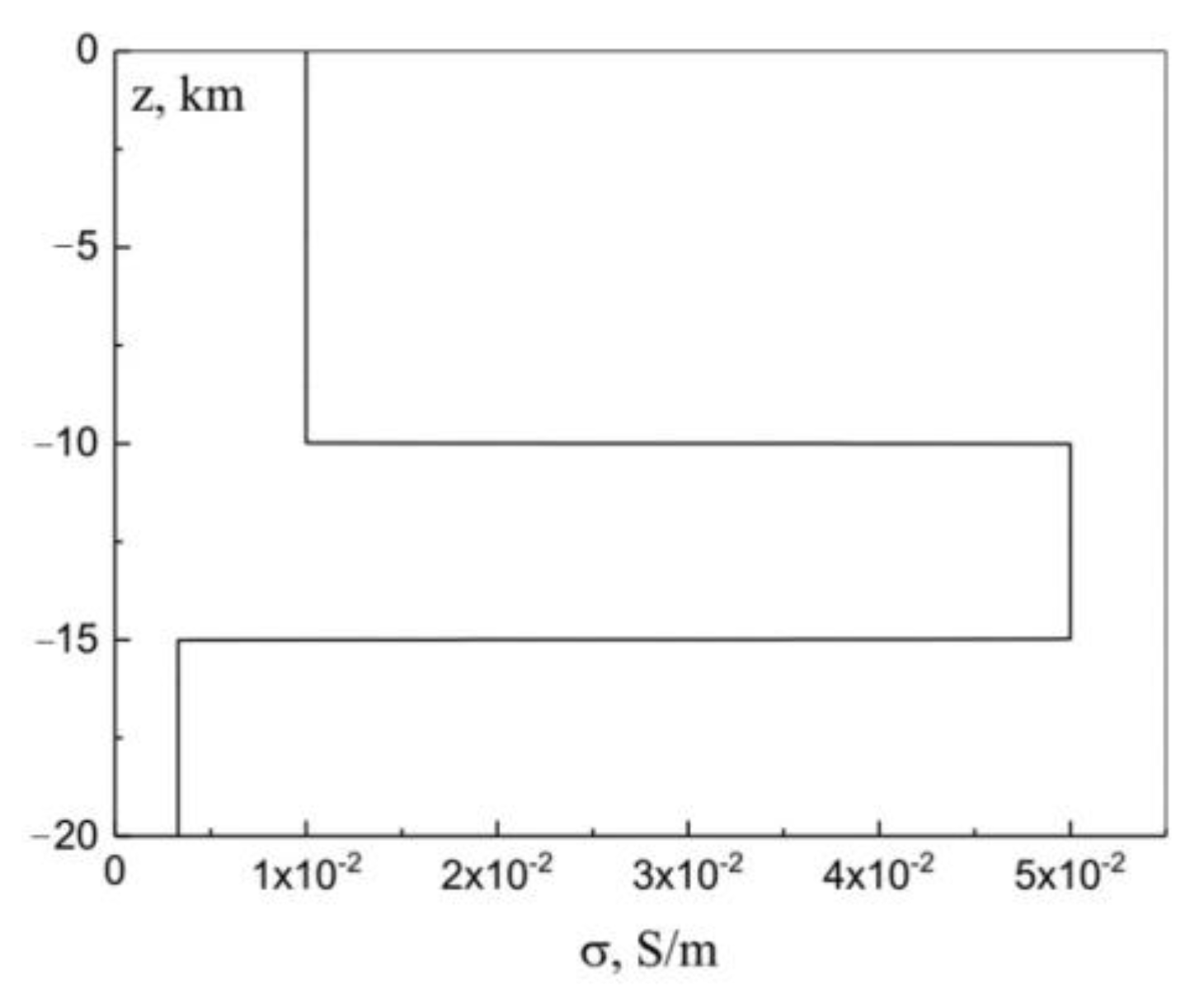
If the characteristic horizontal scale of the change in the conductivity of the earth’s crust exceeds the height of the lower boundary of the ionosphere of the order of 100 km, then it is possible to introduce a local dependence of the conductivity of the earth’s crust σ g ( z ) on the vertical coordinate. The model of layered inhomogeneous conductivity of the earth’s crust used for numerical study is shown in Figure 2.
In the quasi-1-D approximation the Maxwell’s equations lead to the electric field perturbation equation:
2 e z 2 μ 0 σ g ( z ) e t = 0
The system of Equations (6)–(12) makes it possible to find the perturbation of the electric field that occurs as a result of a non-stationary change in the ionosphere conductivity under an influence of its ionization by solar flare radiation.

3. Solution of Electric Field Perturbation Equations

We find the perturbation of the electric field in the atmosphere-ionosphere system. The solution of Equation (9) in the upper ionosphere above the conducting layer in the form of an upwardly propagating wave is determined by the expressions:
e x = e x ( z 1 , t z z 1 u | s i n I | ) ;   e y = e y ( z 1 , t z z 1 u )
In a non-conductive atmosphere in the height interval of 0 < z < z 1 , from Equation (10) we have the following solution:
e ( z , t ) = E 0 ( t ) + E 1 ( t ) z z 1
Between the atmosphere and the upper ionosphere there is a thin layer with Pedersen and Hall conductivities. Integrating Equation (6) over the thickness of this layer, we obtain the boundary conditions on the conducting ionosphere for the tangential components of the electric field disturbance:
{ e } = 0 ,   { e z } μ 0 t ( Σ ^ h e ) = μ 0 t ( Σ ^ h E e x t ) ,   Σ ^ h ( t ) = ( Σ P ( t ) s i n 2 I Σ H ( t ) s i n I Σ H ( t ) s i n I Σ P ( t ) ) ,
where Σ P и Σ H are the integral Pedersen and Hall conductivities of the ionosphere, and curly brackets denote the jump of the corresponding value when passing through the thin ionosphere. Substituting Equations (13) and (14) into the boundary conditions (15), we obtain the Equation for the electric field in the ionosphere E i = E 0 + E 1 at z = z 1 in the following form:
d d t ( Σ e E i ) + 1 μ 0 z 1 E i 1 μ 0 z 1 E 0 = d Σ h ( t ) d t E e x t ,
where Σ e ( t ) = ( Σ e a ( t ) Σ H ( t ) s i n I Σ H ( t ) s i n I Σ e m ( t ) ) ;   Σ e a = Σ P ( t ) s i n 2 I + 1 μ 0 u | s i n I | ;   Σ e m = Σ P ( t ) + 1 μ 0 u .
In the approximation of a perfectly conducting Earth, ( 0 , t ) = E 0 ( t ) 0 . In this case, the system of ordinary differential Equation (16) makes it possible to determine the perturbations of electric and magnetic fields as a result of a nonstationary change in the conductivity of the ionosphere by a solar flare throughout the space. In the case of the earth’s crust with conductivity σ g ( z ) , the distribution of the electric field in the lithosphere is determined from Equation (12). The connection between the electric fields on the Earth’s surface E 0 ( t ) and in the ionosphere E i ( t ) is obtained in the Appendix A, Equation (A2):
E 0 ( t ) = 0 t G ( t t ) E i ( t ) d t
where the kernel of the convolution operator G(t) depends on the vertical distribution of conductivity σ g ( z ) . The algorithm for its calculation is given in Appendix A. The system of equations and boundary conditions that determine the telluric electric field is obtained from (12), (14) and the continuity condition for the tangential component of the electric field and its normal derivative when passing through the Earth’s surface:
2 e z 2 μ 0 σ g ( z ) e t = 0 ;   < z < 0 e ( 0 , t ) = E 0 ( t ) ,   e ( , t ) = 0 ,   e ( z , t ) z | z = 0 = E 1 ( t ) z 1 ,   e ( z , 0 ) = 0
Substituting (17) into (16), we obtain a system of equations that determine the perturbation of the electric field in the ionosphere E i ( t ) :
d E i d t + [ Ω ^ 0 ( t ) + Ω ^ 1 ( t ) ] E i Ω ^ 0 ( t ) 0 t G ( t t ) E i ( t ) d t = Ω ^ 2 ( t ) E e x t
The explicit form of the matrices in the system of Equation (19) is given in Appendix B, Equations (A9) and (A10). Solving the system of Equation (19) and determining by Equation (17) the time dependence of the electric field perturbation on the Earth’s surface, it is possible to calculate its spatiotemporal dependence in the Earth. It is determined from the solution of the boundary value problem (18). The perturbation of the electric current density in the earth’s crust j and the specific power of heat release q by this current are determined by the electric field according to the formulas:
j ( z , t ) = σ g ( z ) E ( z , t ) ;   q ( z , t ) = σ g ( z ) | E ( z , t ) | 2
Equations (19) and (20) make it possible to calculate the space-time distribution of the electric current density on the Earth’s surface, generated by the absorption of ionizing radiation from solar flares in the ionosphere.

4. Model of Perturbation of Integral Conductivities of the Ionosphere

Equation (19) is used to calculate the electric field. The coefficients of this equation are determined by the dependence of the integral conductivities Σ P ( t ) ,   Σ H ( t ) which is a result of ionization of the conducting ionosphere layer by the ionizing radiation of a solar flare. To estimate the characteristics of the electric field and telluric current, we will employ the model of ionosphere ionization by a flat mono-energetic X-ray flux with energy of the flare spectrum maximum, which is absorbed in the lower ionosphere. Its absorption results in an additional ionization of the conducting layer. The time-averaged ionization rate Q ( z ) of a radiation pulse from an isothermal atmosphere at a point in an illuminated hemisphere with latitude ψ and longitude φ is determined by the Chapman’s equation [32]:
Q ( ψ , φ , z , δ ) = Q m   e x p [ 1 z z m H e x p ( z z m H ) ] ,   Q m = C W e H c o s   χ
where H is a homogeneous atmosphere height, W is time-integrated flare energy flux, z m = H ln ( H / l 0 c o s   χ ) ,   l 0 is a radiation quantum path at sea level, C = 1.89 × 10 17 J 1 , χ—zenith angle of the Sun, determined by the expression:
c o s   χ = s i n   ψ   s i n   δ + c o s   ψ   c o s   δ   c o s ( φ φ 0 )
where ψ , φ —latitude and longitude, φ 0 —longitude of the subsolar meridian, δ —angle of declination of the Sun, which is approximately determined by the Equation from [33] (see Figure 1):
δ = 0.41 c o s [ 2 π 365 ( N + 10 ) ]
where 0 N < 365 —number of the day of the year, and N = 0 , corresponds to January 1.
The length of the X-ray quantum path l 0 depends on its energy. It was calculated using the database [34]. The X-ray maximum is located at the height of the conductive layer. For the model of a thin conductive layer located at a height of z = z 1 , characterized by integral conductivities, the Equation (21) makes it possible to obtain the horizontal distribution of the ionization rate of this layer. Assuming z 1 = z m and substituting (22) into (21), we get:
Q ( ψ , φ , z m , δ ) = C W e H [ s i n   ψ   s i n   δ + c o s   ψ   c o s   δ   c o s ( φ φ 0 ) ]
Since the Pedersen and Hall conductivities are mainly determined by the electron concentrations n, then at the height of the thin conducting ionosphere we will assume Σ H ~ n ( z 1 ) ,   Σ P ~ n ( z 1 ) . Therefore, perturbed Σ P ( t ) ,   Σ H ( t ) and unperturbed Σ P 0 ,   Σ H 0 integral conductivities are determined by the formulas:
Σ P ( t ) = Σ P 0 n 0 ( z 1 ) n ( z 1 , t ) ;   Σ H ( t ) = Σ H 0 n 0 ( z 1 ) n ( z 1 , t ) ,
where: n ( z 1 , t ) is the electron concentration in the conducting layer of the ionosphere perturbed by ionizing radiation, n 0 ( z 1 ) = n ( z 1 , t = 0 ) is the electron concentration in the conducting layer of the ionosphere under calm conditions. The electron concentration in the lower ionosphere is determined from the equation of ionization-recombination balance:
d n ( z 1 , t ) d t = q ( z 1 , t ) α ( z 1 ) n 2 ( z 1 , t )
where q ( z 1 , t ) is the ionization rate of lower ionosphere, α ( z 1 ) is a coefficient of electron-ion recombination in the lower ionosphere. Let us represent the ionization rate of the lower ionosphere as the sum of its stationary value q 0 and the perturbation q 1 ( t ) , caused by the ionizing radiation pulse of the solar flare: q = q 0 + q 1 ( t ) . Therefore, denoting the change in the electron concentration as a result of additional ionization n 1 ( t ) = n ( t ) n 0 compared to its stationary value, from Equation (26) we obtain:
d n 1 ( t ) d t = q 1 ( t ) 2 α n 0 n 1 ( t ) α n 1 2 ( t ) ;   n 0 = q 0 α
From Equation (25) we obtain expressions for the integral conductivities:
Σ P ( t ) = Σ P 0 [ 1 + n 1 ( t ) n 0 ] ;   Σ H ( t ) = Σ H 0 [ 1 + n 1 ( t ) n 0 ]
For short flashes, the duration of which is shorter than the duration of the change in the field and current, the Equation (27) has an analytical solution. In this case, we choose the time dependence of the perturbation of the ionization rate in the form of a delta function:
q 1 ( t ) = Q δ ( t )
Substituting Equation (29) into Equation (27), we obtain the equation for the moments of time t > 0 and the initial condition at t = + 0 :
d n 1 ( t ) d t = 2 α n 0 n 1 ( t ) α n 1 2 ( t ) ;   n 1 ( t = + 0 ) = Q
The solution of Equation (30) has the form:
n 1 ( t ) = 2 n 0 1 ( 1 2 n 0 Q ) e x p ( 2 α n 0 t )
Substituting Equation (31) into Equation (28), we obtain the time dependence of the components of the integral conductivity of the lower ionosphere as a result of absorption of a pulsed ionizing radiation flux in it:
Σ p ( t ) = Σ p 0 [ 1 + 2 1 ( 1 2 n 0 Q ) e x p ( 2 α n 0 t ) ] ;   Σ H ( t ) = Σ H 0 [ 1 + 2 1 ( 1 2 n 0 Q ) e x p ( 2 α n 0 t ) ]
From Equation (32) it follows that at the initial moment t = +0, the integral conductivity changes abruptly to the value:
Σ P ( t = + 0 ) Σ P 0 = Σ H ( t = + 0 ) Σ H 0 = 1 + Q n 0
At t the integral conductivity tends to a stationary value according to the law:
Σ P ( t ) Σ P 0 = Σ H ( t ) Σ H 0 = 1 2 Q Q 2 n 0 e x p ( 2 α n 0 t )
The dependence of integral conductivities on latitude and longitude Σ P , H ( ψ , φ , t ) is determined by the corresponding dependence of the ionization rate Q(ψ, φ) according to Equation (32). Substituting Equation (32) into Equation (A10), we obtain the coefficients of Equation (19), the solution of which makes it possible to calculate the characteristics of the electric field and telluric current resulting from the absorption of ionizing radiation from solar flares in the ionosphere.

5. Results of Estimation of Telluric Current Parameters

For estimation of telluric current, the databases of the spatial distribution of the integral conductivities of the ionosphere and the electric field in it were formed. The following Internet resources were used [35,36,37]:
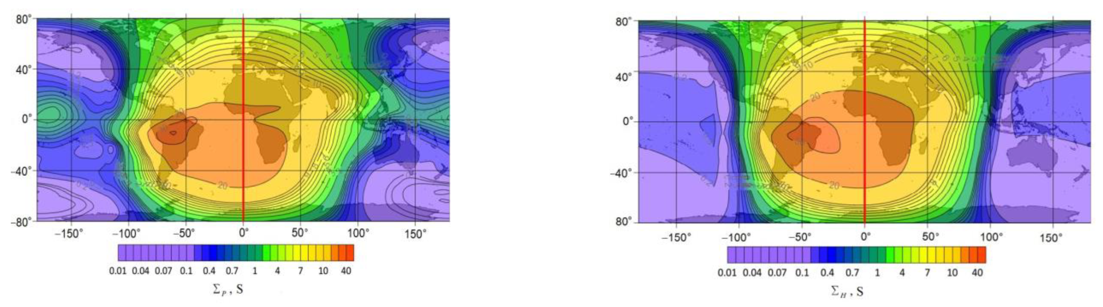
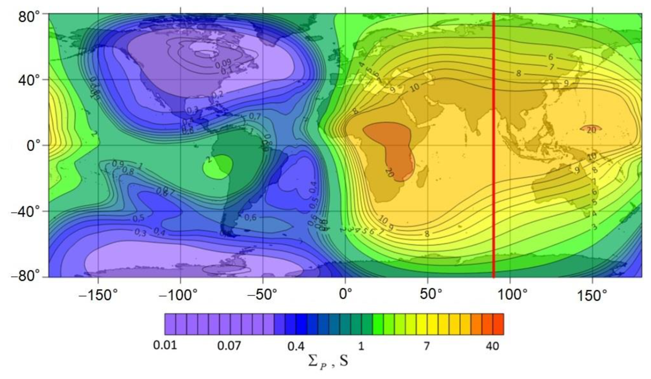
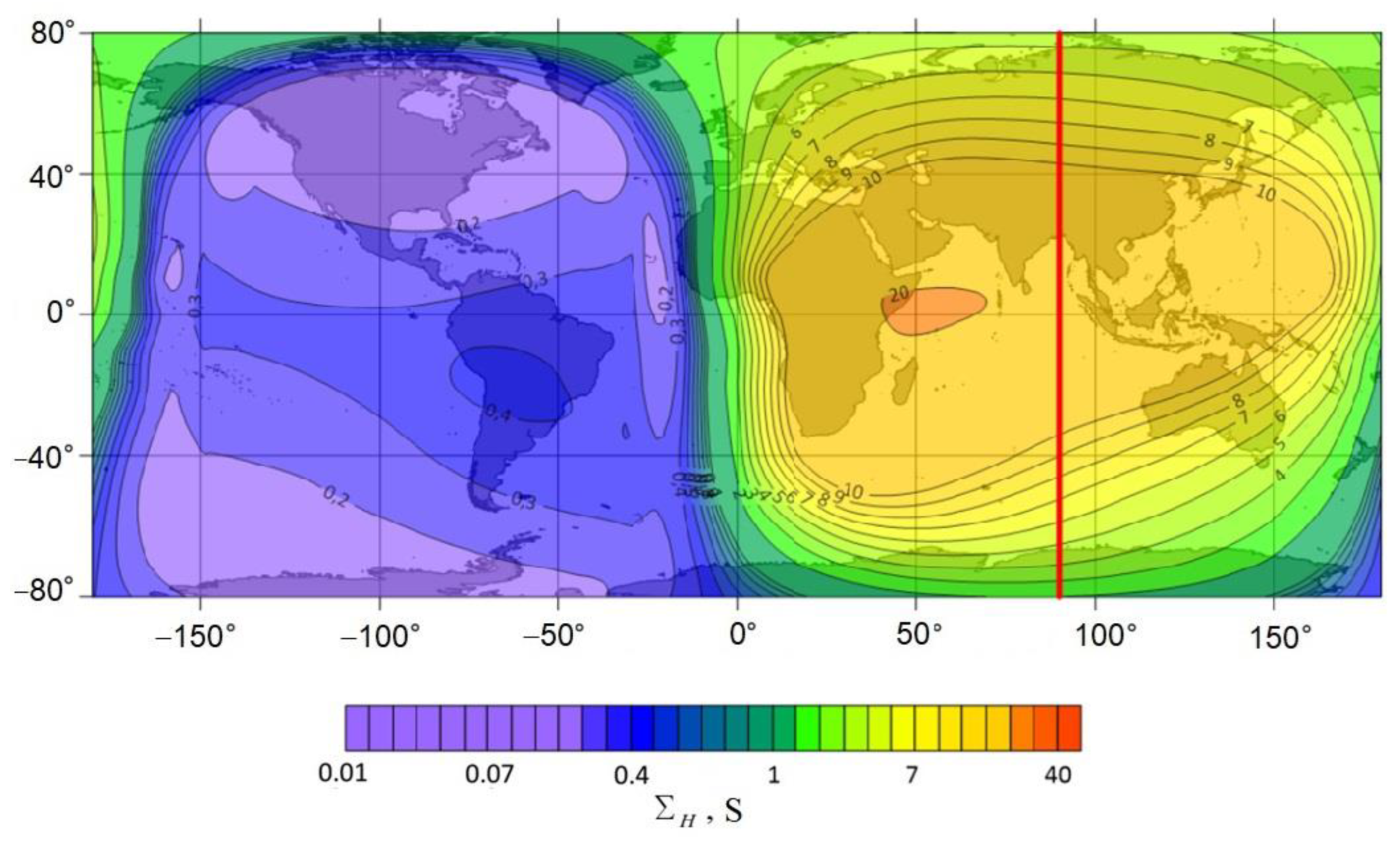
Figure 3 shows the global spatial distribution of the integrated Pedersen and Hall conductivities in the latitude range −80–80° for the universal time 12UT. The red vertical line shows the position of the subsolar meridian.
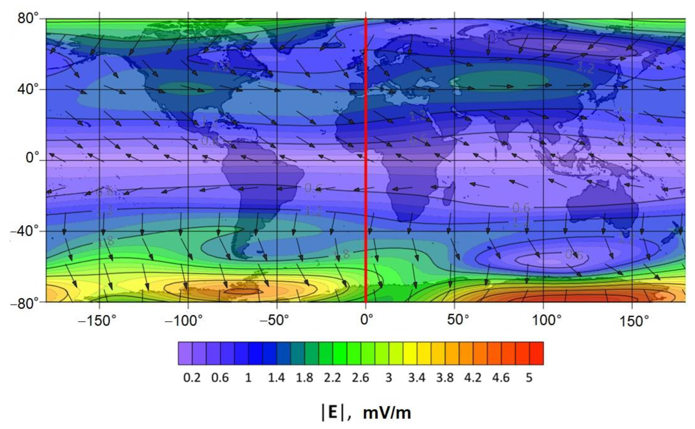
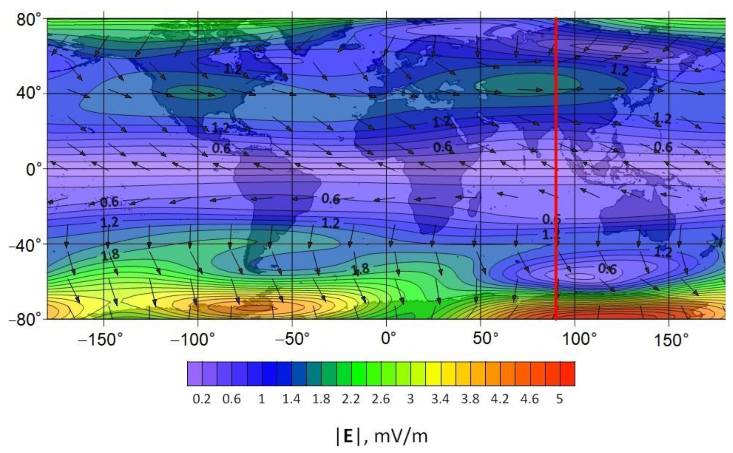
Figure 4 shows the spatial distribution of the amplitude of the electric dynamo field and its vector in the lower ionosphere for the same parameters.
Calculations of the disturbance of electromagnetic field and current were made using the model described in Section 2, Section 3 and Section 4 and Appendix A and Appendix B. They were carried out using the Wolfram Mathematica system for analytical and numerical calculations. In most cases, the built-in tools of the system were used, such as procedures for analytical operations with matrices and the numerical solution of differential equations, both ordinary and with partial derivatives. The procedure for the numerical inversion of the Laplace transform was carried out using the Stehfest algorithm (see Appendix A for details). The calculations were carried out for the San Andreas fault area (USA, California) with coordinates 35°07′ N; 119°39′ W. The fault is oriented at an angle of approximately φ = 30° to the meridian. All the background parameters of the environment necessary for the calculations were determined using databases obtained from the Internet resources mentioned above. In addition, according to [38], the recombination coefficient α = 10−13 m3. The value of the time-integrated flare energy flux density W = 0.005 J/m2 was also chosen. The calculations were carried out for the date 20.07.2020 and two moments of universal time: 15:00 UT and 18:00 UT. Environment parameters are shown in Table 1.
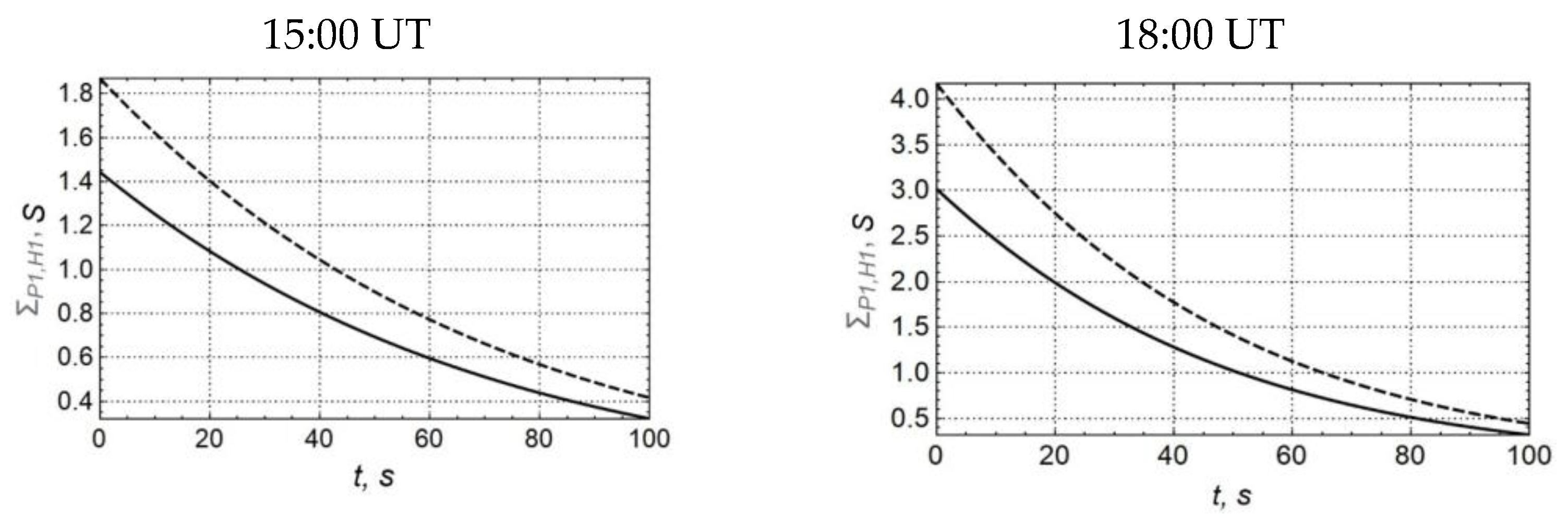
Below are graphs illustrating the results of calculations of the time dependences of disturbances in the Hall and Pedersen conductivities of the ionosphere, the components of the electric current density, its absolute value, as well as the hodograph of the current density vector.
The following conclusions may be drawn from the calculation results. 
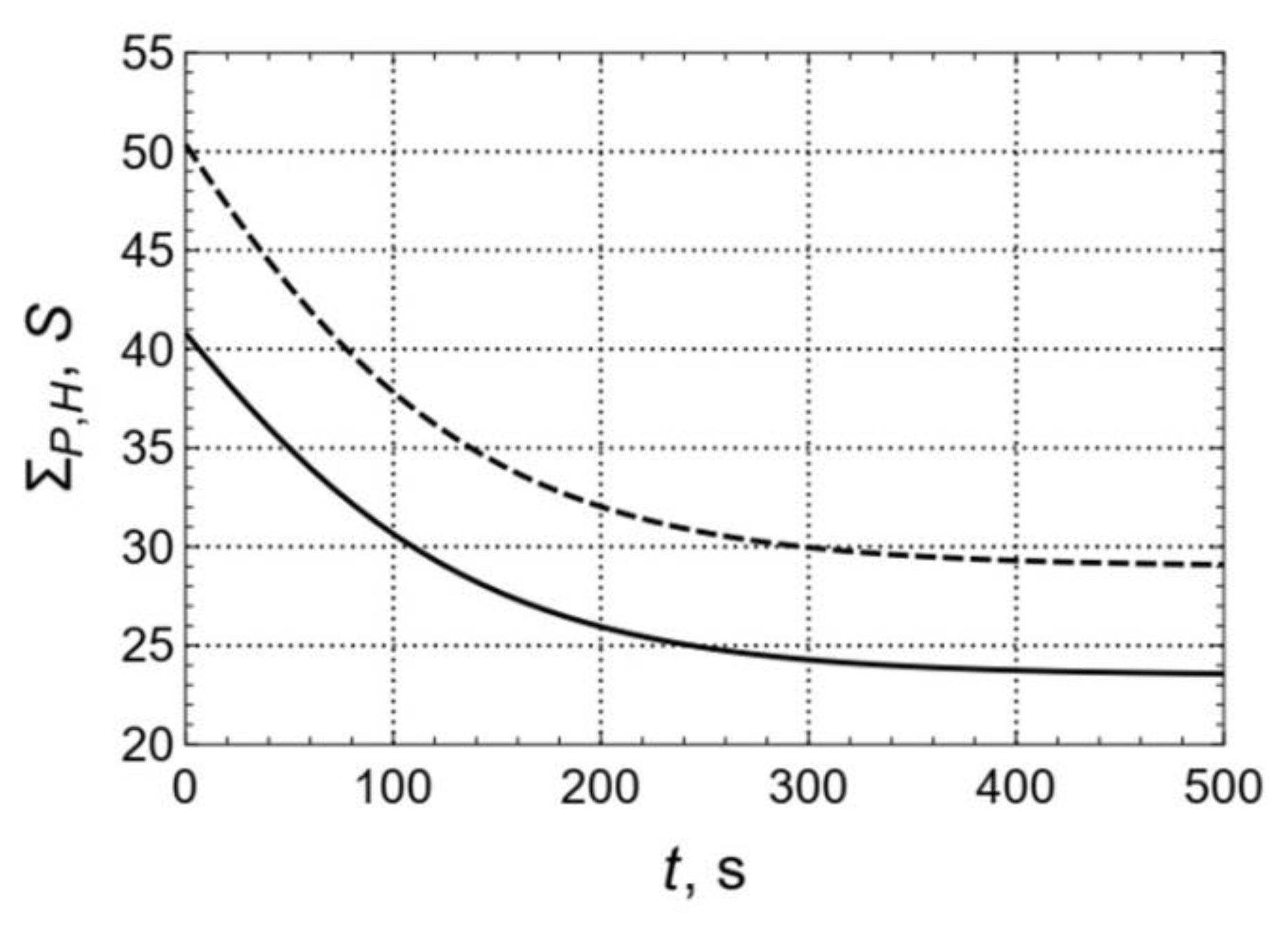
Figure 5 demonstrates that the perturbations of the integral ionosphere conductivities reach about 2 S for 15UT and 4 S for 18UT. At the same time, their relaxation time is about 40–50 s and somewhat less for 18UT, which is explained by the higher value of the background electron concentration.
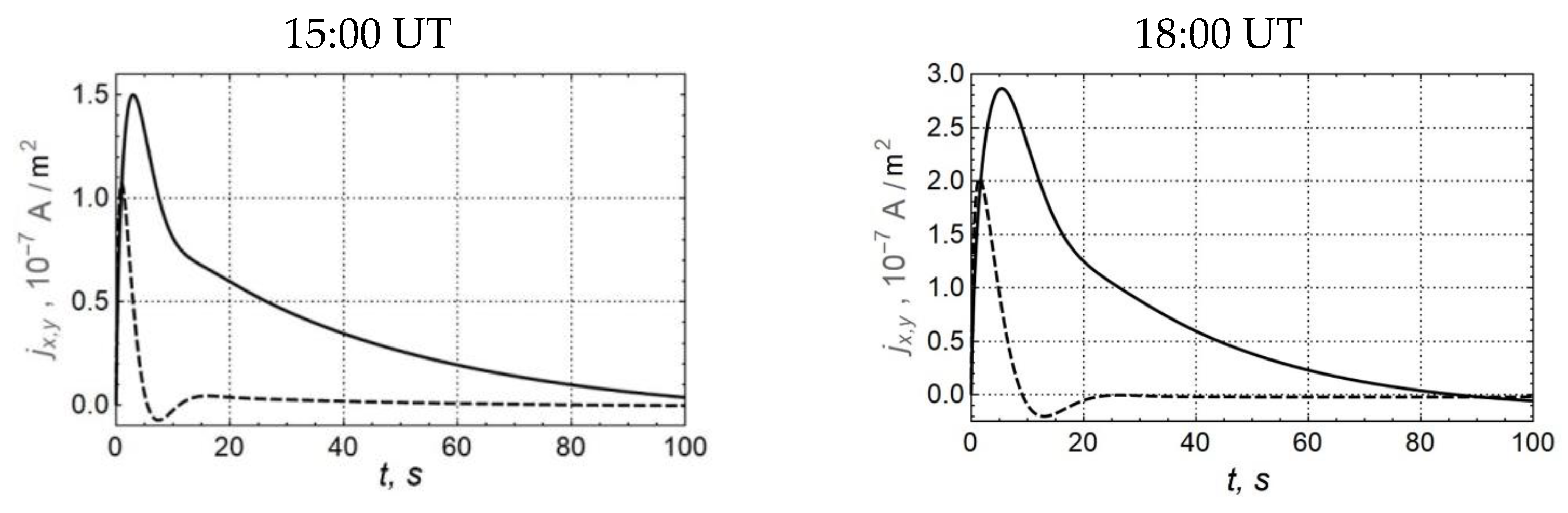
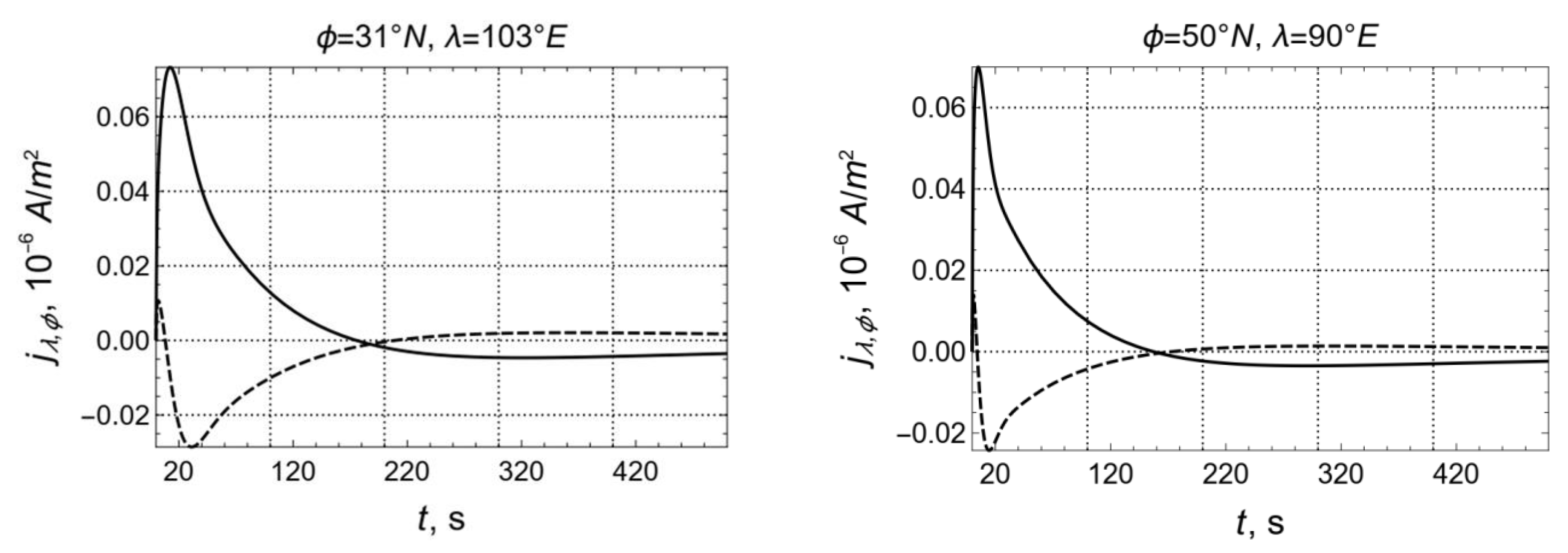
The duration and, to a lesser extent, the amplitude of the pulse of the j x component oriented along the geomagnetic meridian is greater than that of the j y component (see Figure 6). There is a small oscillatory component in the time dependence of the j y component, which is explained by the Hall current effects in the ionosphere.
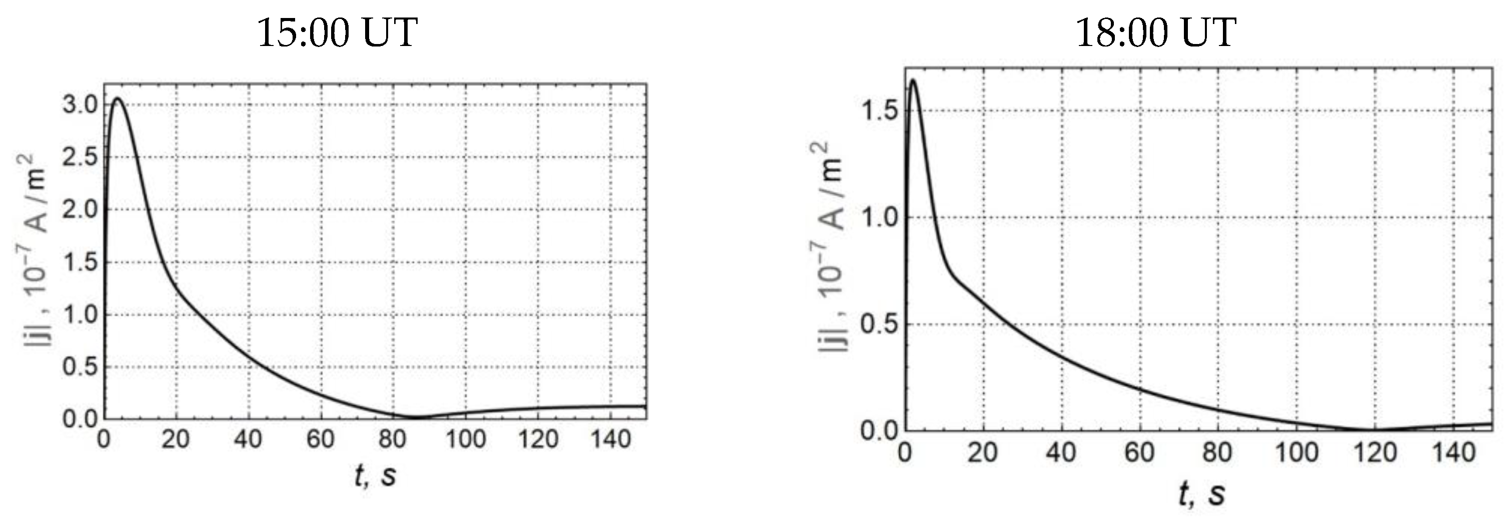
The amplitude of the current density reaches 1.5·10−7 A/m2 for 15:00 UT and 3·10−7 A/m2 for 18:00 UT, increasing similarly to the conductivity perturbation by 2 times (Figure 7). The duration of the current density pulse is 10 to 40 s, and it is longer for 18:00 UT, that is explained by the large values of the integral conductivities of the ionosphere.
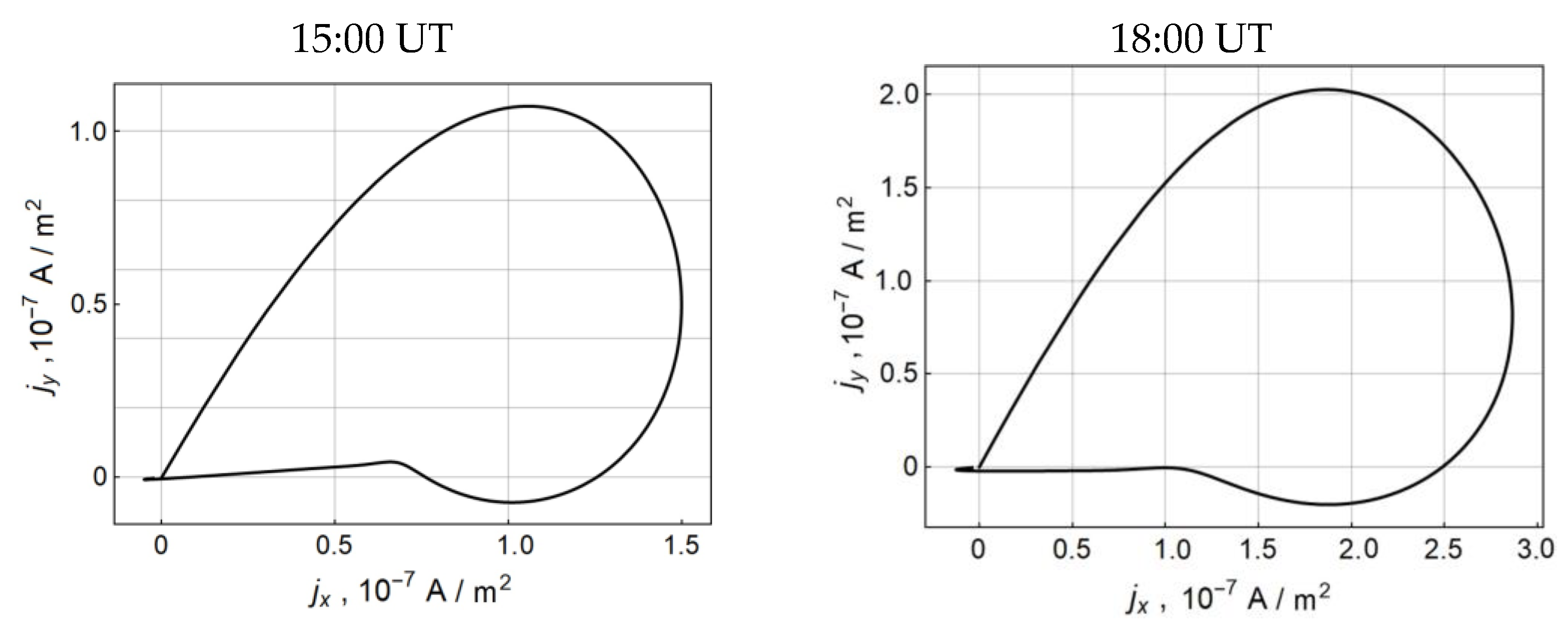
Figure 8 shows the hodograph vectors of the telluric current density at 15:00 UT and 18:00 UT.

6. Calculation of the Spatial Distribution of the Telluric Current

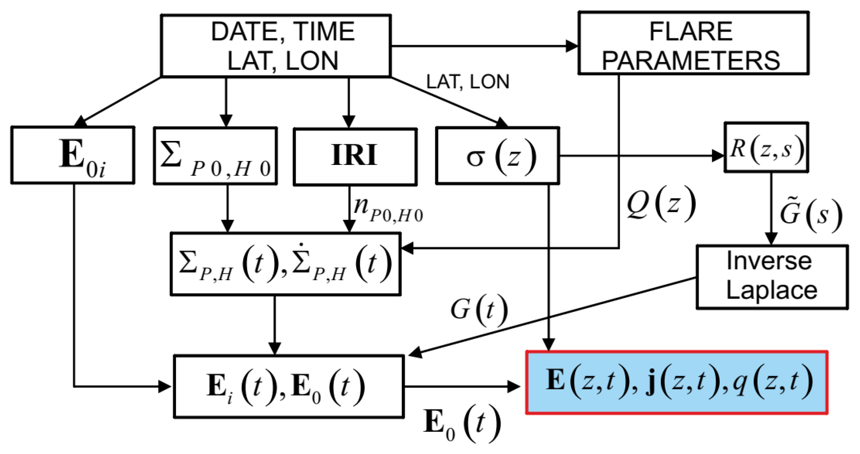
The calculation was performed with employment of the developed software package, which consists of several parts [39,40], a code written in C++ (see the flowchart in Figure 9) and an external software module written in the system [41] incorporated into a single computer code.
The code starts its operation upon receipt of the following initial data: date, time, and power of the solar flare. Based on these initial data the code calculates the subsolar point, and the background parameters of the ionosphere at altitudes of 100 and 140 km, the Pedersen and Hall conductivities, and also builds a model of the earth’s electric field according to Volland [42,43,44]. With employment of the IGRF (International Reference Geomagnetic Field) model [39], which is a series of mathematical models of the Earth’s main field and its annual rate of change (secular course), the main parameters of the magnetic field at a specified point in time are calculated. Further, according to the IRI (International Reference Ionosphere) model [40], the electron density, electron temperature, ion temperature, ionic composition (O+, H+, He+, N+, NO+, O+2, cluster ions), equatorial vertical ion drift, vertical electron content in the ionosphere, probability F1, propagation probability F, aurora boundaries, an influence of ionospheric storms on the peak densities of F and E are calculated. Then, surface conduction currents are calculated based on the Earth’s conductivity profile in the subsolar region. Based on these calculations the current depth profile is constructed.
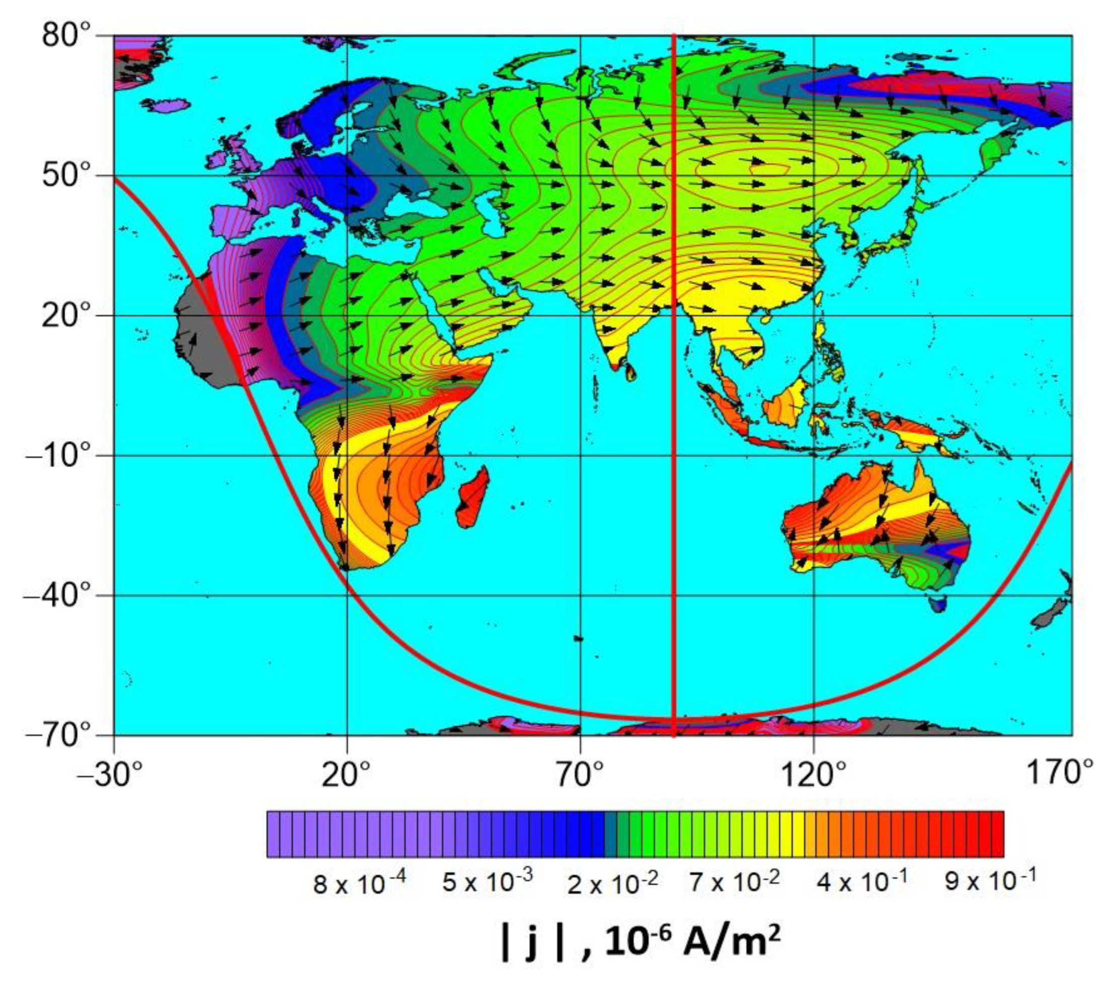
The calculations were made for the following parameter values: date—19 June 2020, time—06:00 UT (longitude of the subsolar meridian 90°), height of the conducting layer of the ionosphere is 120 km, time-integrated flare energy flux density is 0.005 J/m2 (strong solar flare of X-class). As a result of mathematical modeling, the results of numerical modeling are shown in Figure 10, Figure 11, Figure 12, Figure 13, Figure 14, Figure 15, Figure 16 and Figure 17.

7. Discussion

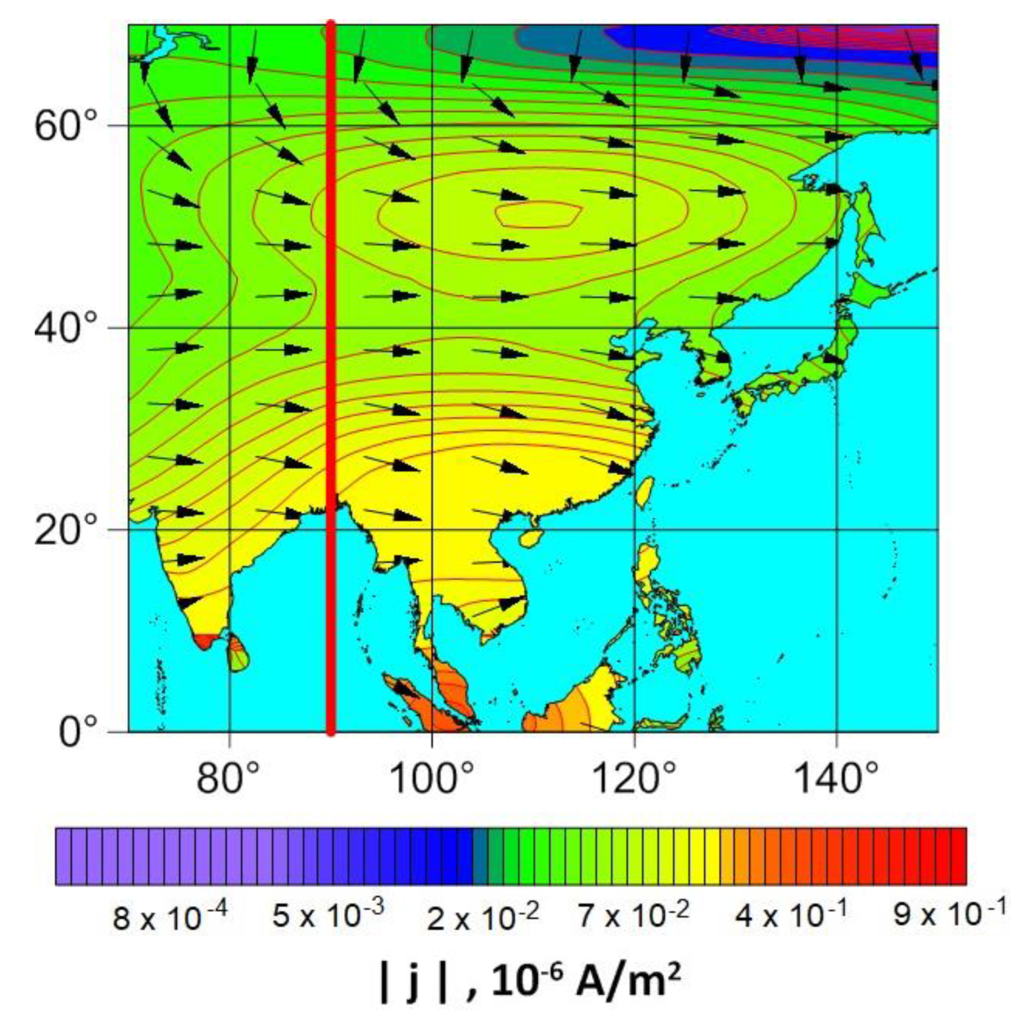
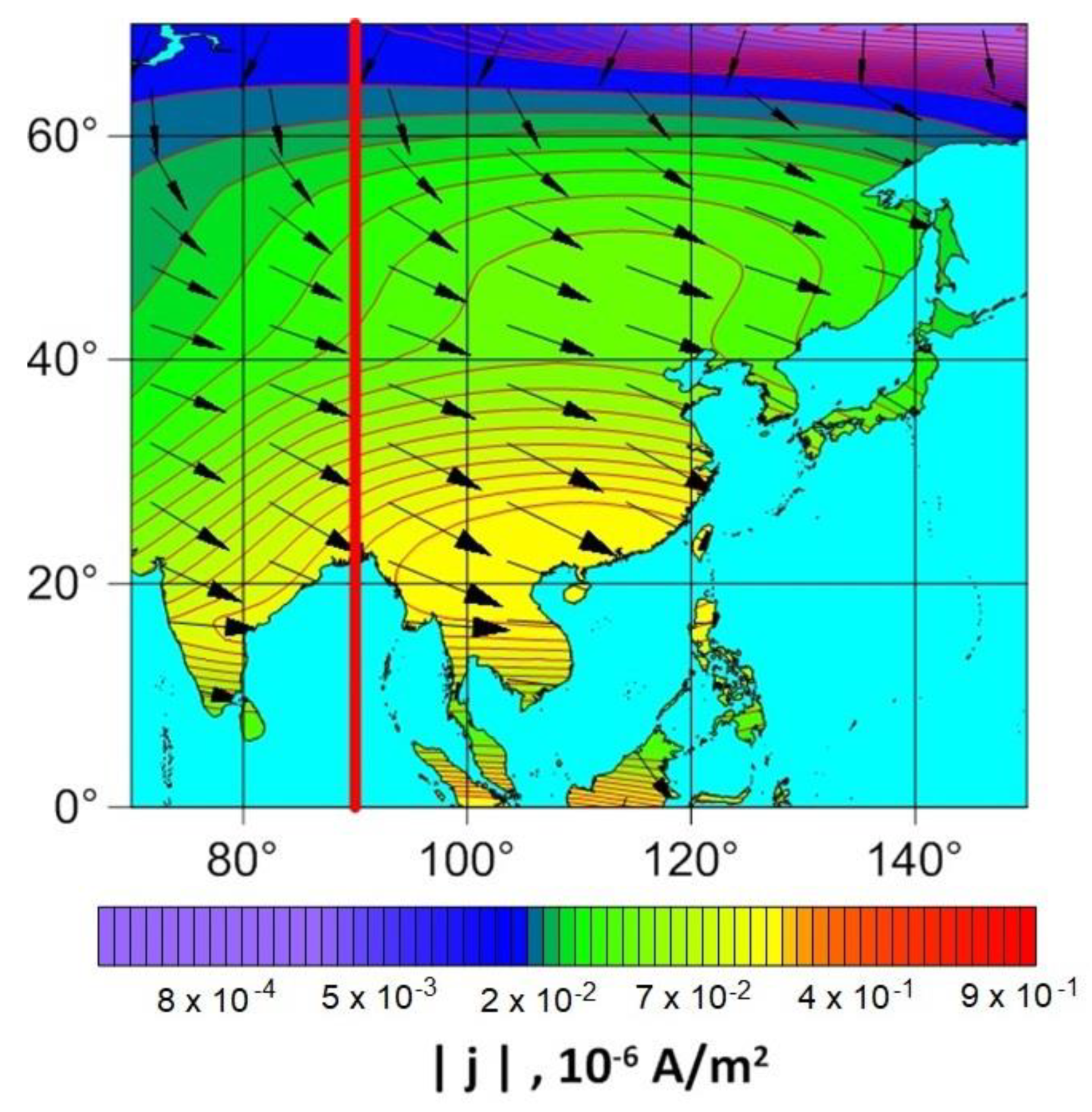
The results of numerical estimations obtained with developed model and computer code indicate that after the solar flare of X-class the telluric current density in the conductive layer of lithosphere may reach 10−8–10−6 A/m2 (Figure 14, Figure 15 and Figure 16), the current pulse duration is about 100 s, and the current front duration is 10 s (Figure 17). These values are 2–3 orders more than average telluric current density of 2·10−10 A/m2 in lithosphere [45] and are comparable with parameters of the electric current pulses generated in the lithosphere by artificial pulsed power sources [29]. It should be noted that these electrical pulses injected into the Earth crust in seismic-prone areas resulted in electromagnetic triggering of weak earthquakes and spatiotemporal re-distribution of regional seismicity of Pamir and Northern Tien Shan. It means that the solar flares provided the time-integrated flare energy flux density over 0.005 J/m2 are capable to trigger earthquakes in the seismic-prone areas as well, as it was supposed in [25,26,46]. This conclusion is supported by the cases of observation of magnetic pulses before earthquake occurrence [47,48] similar to numerical estimations of magnetic pulses generated by X-ray radiation of solar flare and telluric current pulses in conductive layer of lithosphere with employment of developed physical model and computer code (Figure 7 and Figure 17), as well as by the case of sharp increase in global and regional seismicity (Greece) after solar flare of X9.3 class of 6 September 2017 [26]. This effect may be used as a basis of the short-term earthquake prediction with employment of clearly recorded external electromagnetic impacts on the earthquake preparation area.
The concept of earthquake predictability based on triggering phenomena has been formulated in [49]. Based on field observations of behavior of seismicity before the strong earthquakes, as well as laboratory studies of response of acoustic emission (crack formation) from the rock samples under subcritical stress-strain state and external triggering actions. The following algorithm of short-term earthquake prediction based on earthquake triggering phenomena is proposed: “(a) determine the volume of an unstable area (systems of local unstable areas of various scales); (b) monitor the triggering effects and assess their impact on unstable areas; (c) estimate of probability (reasonable, not high) of the place, time, and magnitude of an earthquake” [49].
The first step (a) of this approach may be implemented based on various methods of selection of regions with impending strong earthquakes [49,50,51,52]. For the case of electromagnetic earthquake triggering, in addition, it is important to select the crust faults favorable for generation of maximal telluric current density (orientation and electrical conductivity). It is obvious that the maximal telluric currents will be generated when the current density vector will be parallel to fault direction, rather normal to it.
The numerical results demonstrate that the maximum values of the current density are observed in the southern hemisphere, while the subsolar point (23.5° N, 90° E) is in the northern hemisphere (see Figure 14). Thus, the response of the Earth seismic activity to the strong solar flare with higher probability may be anticipated in the southern hemisphere.
The current density vectors in the northern hemisphere at low and middle latitudes are oriented mainly in the latitudinal direction, and in high latitudes - in the meridional direction. In the southern hemisphere, they are oriented, as a rule, in the meridional direction. It is very important for selection of regions where the response of seismic activity to solar flares will be statistically analyzed. For the increase in the reliability of the statistical analysis, keeping in mind the obtained numerical results on the orientation of the current density vector, only the regions should be considered for statistical study, where the orientation of crust faults coincides with the current density vector. Otherwise, the telluric current density generated in the fault may be not sufficient for electromagnetic triggering of earthquake resulted in false statistical results and conclusions on solar-terrestrial relations when the whole region is analyzed with the faults of various orientations.
Another important aspect for selection of the crust faults sensitive to severe space weather conditions is their electrical conductivity, which is usually determined by magnetotelluric (MT) method [53,54]. The MT results demonstrated that the San Andreas fault [55] and other major faults, namely, the Alpine fault in New Zealand [56] and the Fraser fault in British Columbia, Canada [57] have conductive zones with specific resistance of 0.8 to 50 Ω⋅m. At the same time some major transcurrent faults demonstrated evidence for both conductive and resistive fault zones. For example, the Tintina fault in the northern Cordillera is a major fault [53], where MT results show that the fault is associated with a 20 km wide resistive zone (>400 Ω⋅m) at depths exceeding 5 km. The Denali fault in Alaska is also associated with relatively resistive rocks at upper crustal depths [58], and the San Andreas fault at Carrizo Plain has a resistive zone at midcrustal depths [59]. The resistance of these faults varies within a range of ~250–10,000 Ω⋅m, and, therefore, generation of a splash of telluric currents there due to severe space weather capable to trigger earthquake is impossible.
Thus, based on obtained numerical results, in our opinion, the correct statistical correlation analysis of solar-terrestrial relations should be carried out in the future in the following sequence:
(a)
determination of an unstable area (the crust fault section) where the strong earthquake is anticipated based on existing methods of selection of regions with impending strong earthquakes [49,50,51,52];
(b)
selection of the crust faults in the areas determined in step a) favorable for generation of maximal telluric current density from point of view of their orientation close to direction of the current density vector, as well as their electrical conductivity;
(c)
sampling the earthquakes from regional seismic catalogs which occurred on the faults selected according to step b);
(d)
correlation analysis of earthquake occurrence and variations of space weather parameters.

8. Conclusions

The obtained numerical results demonstrate that solar flares can cause strong pulsed variations in the density of telluric currents in seismogenic conductive faults, which may reach the values comparable to the current densities generated in the Earth’s crust by artificial pulsed DC power sources used for active electromagnetic monitoring resulted in triggering of weak seismicity and spatiotemporal re-distribution of regional seismicity. Consequently, the triggering of seismic events is possible not only by artificial sources of electric current, but also by ionospheric disturbances, such as, for example, strong solar flares and subsequent geomagnetic storms. The presented results may serve as a physical basis for development of a new approach to solving the problem of short-term earthquake prediction based on electromagnetic triggering effects. The developed method and computer code for calculating telluric currents makes it possible to numerically simulate the electromagnetic impact of various space weather phenomena on the Earth crust, resulting in the generation of electric currents in conductive subjects of the lithosphere, such as crust faults.

Author Contributions

Conceptualization, V.S. and V.N.; methodology, V.S. and A.Y.; software, A.Y. and G.M.; validation, formal analysis, investigation, V.S.; resources, data curation, G.M.; writing—original draft preparation, V.S. and A.Y.; writing—review and editing, V.N.; visualization, G.M.; supervision, project administration, funding acquisition, V.N. All authors have read and agreed to the published version of the manuscript.

Funding

This research was funded by Russian Foundation for Basic Research (RFBR) grant No. 21-55-53053.

Institutional Review Board Statement

Not applicable.

Informed Consent Statement

Not applicable.

Data Availability Statement

Not applicable.

Conflicts of Interest

The authors declare no conflict of interest.

Appendix A

Let us use the equation system (18) to express the electric field disturbance on the Earth’s surface E0 through its value at the ionospheric level Ei. Performing the Laplace transform in time, we obtain the equation:
d 2 e ˜ d z 2 = μ 0 σ g ( z ) s e ˜
the solution of which, satisfying the boundary condition at z = 0, has the form:
e ˜ ( z , s ) = E ˜ 0 ( s ) f ( z , s )
In Equation (A2) the following expression is used:
E ˜ 0 ( s ) = 0 E 0 ( t ) e x p ( s t ) d t
The function f ( z , s ) is a solution of the following boundary problem:
d 2 f d z 2 = μ 0 σ g ( z ) s f ;   f ( 0 , s ) = 1 ;   f ( , s ) = 0
From (A3) it follows that the function f ( z , s ) is determined only by the vertical distribution σ g ( z ) of the electrical conductivity of the earth’s crust. Applying the Laplace transform to the boundary condition (18):
E 0 ( s ) d f ( z , s ) d z | z = 0 = E 1 ( s ) z 1 ;   E i ( s ) = E 0 ( s ) + E 1 ( s )
we obtain a relation between the electric field on the Earth’s surface and in ionosphere:
E ˜ 0 ( s ) = E ˜ i ( s ) [ 1 + z 1 d f ( z , s ) d z | z = 0 ] 1
Applying to (A4) the inverse Laplace transform, we obtain an integral transformation for determining the electric field on the Earth’s surface:
E 0 ( t ) = 0 t G ( t t ) E i ( t ) d t
In (A5) the kernel of the integral operator is:
G ( t ) = L 1 [ 1 + z 1 d f ( z , s ) d z | z = 0 ] 1
where the symbol L 1 { } denotes the operation of the inverse Laplace transform. To determine the function G(t), it is necessary to find a solution of the boundary value problem (A3). To solve it, the method of invariant imbedding [60] was used. We transform the Equation (A3) to a system of two first-order equations:
d   f d   z = g ,   d   g d z = q 2   f ;   q 2 ( z , s ) = μ 0 σ g ( z ) s
For the function R = g / f from Equation (A6) the Riccati equation is:
d   R d   z + R 2 = q 2
We assume that dependence of the Earth crust conductivity σ g ( z ) on the vertical coordinate z is given by the function:
σ g ( z ) = { 10 2   S / m ,   0 > z > 10   k m 5 × 10 2   S / m ,   10   k m > z > 15   k m 3.3 × 10 3   S / m ,   15   k m > z > 25   k m 10 3   S / m ,   z < 25   k m
The plot of function σ g ( z ) is shown in Figure 2. To solve the Equation (A7), we choose the boundary condition ( z m ) = q m = μ 0 σ m s . According to Equation (A7), R = c o n s t at z < z m . From the first equation of the system (A6) and boundary condition (A3) we obtain the equation:
d f ( z , s ) d z | z = 0 = R ( 0 , s )
Using the equation, we wright the kernel of integral operator (31) as:
G ( t ) = L 1 [ 1 1 + z 1 R ( z = 0 , s ) ]
Therefore, for calculation of the kernel of integral operator (A5) we found a solution of the Riccati (A7) and substituted into equity (A8). The inverse Laplace transform (A8) was calculated using the Stehfest algorithm described in [61]. This algorithm defines the approximate inverse Laplace transform f(t) of the function f ¯ ( s ) as the following expression:
f ( t ) a n = 1 N K n f ¯ ( n a ) ;   a = ln ( 2 ) / t
with an even number of terms N, usually chosen as 10 to 14. This algorithm provides good results for smooth functions f(t). It was tested on a number of examples of functions whose Laplace transform has an analytical expression, for example, ( t ) = t e x p ( t ) ,   f ¯ ( s ) = 1 / ( 1 + s ) 2 and demonstrated an error not exceeding one percent when choosing N = 10–12. The calculations took into account that the kernel of the operator G(t) has an integrable singularity 1 / t as t → 0. The regularization of the singularity was carried out according to the formula:
G ( t ) G r e g ( t ) = G ( t ) [ 1 e x p ( t 2 / t r e g 2 ) ]
where t r e g = 0.03   s was selected from condition that its value is much less than the characteristic time scales of electromagnetic field.

Appendix B

Coefficients in Equation (18) are:
Ω ^ 0 ( t ) = 1 μ 0 z 1 Σ ^ e 1 ( t ) ;   Ω ^ 1 ( t ) = Σ ^ e 1 ( t ) d Σ ^ e e ( t ) d t ;   Ω ^ 2 ( t ) = Σ ^ e 1 ( t ) d Σ ^ h ( t ) d t
where matrixes Σ ^ e e ( t ) and Σ ^ h ( t ) are defined by Formulas (15) and (16). We give the coefficients of Equation (19) in explicit form:
Ω ^ 0 ( t ) = 1 μ 0 z 1 a ( Ω 11 0 Ω 12 0 Ω 21 0 Ω 22 0 ) ;   Ω ^ 1 ( t ) = 1 a ( Ω 11 1 Ω 12 1 Ω 21 1 Ω 22 1 ) ;   Ω ^ 2 ( t ) = 1 a ( Ω 11 2 Ω 12 2 Ω 21 2 Ω 22 2 )
Matrix elements have the form:
a = Σ e a Σ e m + ( Σ H s i n I ) 2 ;   Ω 11 0 = Σ e m ;   Ω 22 0 = Σ e a ;   Ω 21 0 = Σ H s i n I = Ω 12 0 Ω 11 1 = Σ e m d Σ e a d t + Σ H s i n 2 I d Σ H d t ;   Ω 22 1 = Σ e a d Σ e m d t + Σ H s i n 2 I d Σ H d t Ω 12 1 = 1 s i n I ( Σ e m d Σ H d t Σ H d Σ e m d t ) ;   Ω 21 1 = 1 s i n I ( Σ e a d Σ H d t + Σ H d Σ e a d t ) Ω 11 2 = 1 s i n 2 I ( Σ e m d Σ P d t + Σ H d Σ H d t ) ;   Ω 22 2 = Σ e a d Σ P d t + Σ H s i n 2 I d Σ H d t Ω 12 2 = 1 s i n I ( Σ e m d Σ H d t Σ H d Σ P d t ) ;   Ω 21 2 = 1 s i n I ( Σ e a d Σ H d t + Σ H s i n 2 I d Σ P d t )

References

  1. Freed, A.M. Earthquake triggering by static, dynamic, and postseismic stress transfer. Annu. Rev. Earth Planet. Sci. 2005, 33, 335–367. [Google Scholar] [CrossRef] [Green Version]
  2. Scuderi, M.; Collettini, C. The role of fluid pressure in induced vs. triggered seismicity: Insights from rock deformation experiments on carbonates. Sci. Rep. 2016, 6, 24852. [Google Scholar] [CrossRef] [Green Version]
  3. Zhang, Z.; Wu, S.; Li, J. The solar and lunar effect of earthquake duration and distribution. Earthq. Sci. 2013, 26, 117–124. [Google Scholar] [CrossRef] [Green Version]
  4. Brodsky, E.E.; Mori, J.J.; Anderson, L.; Chester, F.M.; Conin, M.; Dunham, E.M.; Eguchi, N.; Fulton, P.M.; Hino, R.; Hirose, T.; et al. The State of Stress on the Fault Before, During, and After a Major Earthquake. Annu. Rev. Earth Planet. Sci. 2020, 4, 2.1–2.26. [Google Scholar] [CrossRef]
  5. Anagnostopoulos, G.; Spyroglou, I.; Rigas, A.; Preka-Papadema, P.; Mavromichalaki, H.; Kiosses, I. The sun as a significant agent provoking earthquakes. Eur. Phys. J. Spec. Top. 2021, 230, 287–333. [Google Scholar] [CrossRef]
  6. Lee, H.D.P. Aristotle Meteorologica; Harvard University Press: Cambridge, MA, USA, 1952; 480p. [Google Scholar]
  7. Wolf, R. On the periodic return of the minimum of sun-spots: The agreement between those periods and the variations of magnetic declination. Philos. Mag. 1853, 5, 67. [Google Scholar] [CrossRef]
  8. Simpson, J.F. Solar activity as a triggering mechanism for earthquakes. Earth Planet. Sci. Lett. 1967, 3, 417–425. [Google Scholar] [CrossRef]
  9. Gribbin, J. Relation of sunspot and earthquake activity. Science 1971, 173, 558. [Google Scholar] [CrossRef] [PubMed]
  10. Meeus, J. Sunspots and earthquakes. Phys. Today 1976, 29, 11. [Google Scholar] [CrossRef]
  11. Odintsov, S.; Boyarchuk, K.; Georgieva, K.; Kirov, B.; Atanasov, D. Long-period trends in global seismic and geomagnetic activity and their relation to solar activity. Phys. Chem. Earth 2006, 31, 88–93. [Google Scholar] [CrossRef]
  12. Tavares, M.; Azevedo, A. Influence of solar cycles on earthquakes. Nat. Sci. 2011, 3, 436–443. [Google Scholar] [CrossRef] [Green Version]
  13. Sobolev, G.A.; Zakrzhevskaya, N.A.; Kharin, E.P. On the relation between seismicity and magnetic storms. Izv. Phys. Solid Earth 2001, 37, 917–927. [Google Scholar]
  14. Zakrzhevskaya, N.A.; Sobolev, G.A. On the seismicity effect of magnetic storms. Izv. Phys. Solid Earth 2002, 38, 249–261. [Google Scholar]
  15. Urata, N.; Duma, G.; Freund, F. Geomagnetic Kp Index and Earthquakes. Open J. Earthq. Res. 2018, 7, 39–52. [Google Scholar] [CrossRef] [Green Version]
  16. Sobolev, G.A. The effect of strong magnetic storms on the occurrence of large earthquakes. Izv. Phys. Solid Earth 2021, 57, 20–36. [Google Scholar] [CrossRef]
  17. Duma, G.; Ruzhin, Y. Diurnal changes of earthquake activity and geomagnetic Sq-variations. Nat. Hazards Earth Syst. Sci. 2003, 3, 171–177. [Google Scholar] [CrossRef] [Green Version]
  18. Rabeh, T.; Miranda, M.; Hvozdara, M. Strong earthquakes associated with high amplitude daily geomagnetic variations. Nat. Hazards 2010, 53, 561–574. [Google Scholar] [CrossRef]
  19. Florindo, F.; Alfonsi, L. Strong earthquakes and geomagnetic jerks: A cause/effect relationship? Ann. Geofis. 1995, 38, 457–461. [Google Scholar] [CrossRef]
  20. Florindo, F.; Alfonsi, L.; Piersanti, A.; Spada, G.; Marzocchi, W. Geomagnetic jerks and seismic activity. Ann. Geofis. 1996, 39, 1227–1233. [Google Scholar] [CrossRef]
  21. Tarasov, N.T. Effect of Solar Activity on Electromagnetic Fields and Seismicity of the Earth. IOP Conf. Ser. Earth Environ. Sci. 2021, 929, 012019. [Google Scholar] [CrossRef]
  22. Shestopalov, I.P.; Kharin, E.P. Relationship between solar activity and global seismicity and neutrons of terrestrial origin. Russ. J. Earth Sci. 2014, 14, ES1002. [Google Scholar] [CrossRef] [Green Version]
  23. Marchitelli, V.; Harabaglia, P.; Troise, C.; De Natale, G. On the Correlation between Solar Activity and Large Earthquakes Worldwide. Sci. Rep. 2020, 10, 11495. [Google Scholar] [CrossRef] [PubMed]
  24. Shestopalov, I.P.; Sobolev, G.A.; Kharin, E.P. Implications of solar flares for the seismic activity of the Earth. Izv. Phys. Solid Earth 1998, 34, 603–607. [Google Scholar]
  25. Sorokin, V.M.; Yashchenko, A.K.; Novikov, V.A. A possible mechanism of stimulation of seismic activity by ionizing radiation of solar flares. Earthq. Sci. 2019, 32, 26–34. [Google Scholar] [CrossRef]
  26. Novikov, V.; Ruzhin, Y.; Sorokin, V.; Yaschenko, A. Space weather and earthquakes: Possible triggering of seismic activity by strong solar flares. Ann. Geophys. 2020, 63, PA554. [Google Scholar] [CrossRef]
  27. Akhoondzadeh, M.; De Santis, A. Is the Apparent Correlation between Solar-Geomagnetic Activity and Occurrence of Powerful Earthquakes a Casual Artifact? Atmosphere 2022, 13, 1131. [Google Scholar] [CrossRef]
  28. Love, J.J.; Thomas, J.N. Insignificant solar-terrestrial triggering of earthquakes. Geophys. Res. Lett. 2013, 40, 1165–1170. [Google Scholar] [CrossRef]
  29. Zeigarnik, V.A.; Bogomolov, L.M.; Novikov, V.A. Electromagnetic Earthquake Triggering: Field Observations, Laboratory Experiments, and Physical Mechanisms—A Review. Izv. Phys. Solid Earth 2022, 58, 30–58. [Google Scholar] [CrossRef]
  30. Ratcliffe, J.A. Physics of the Upper Atmosphere; Academic Press: New York, NY, USA, 1960; p. 586. [Google Scholar]
  31. Alfvén, H.; Fälthammar, C.-G. Cosmical Electrodynamics: Fundamental Principles; Clarendon Press: Oxford, UK, 1963; p. 228. [Google Scholar]
  32. Ratcliffe, J.A. An Introduction to the Ionosphere and Magnetosphere; University Press: Cambridge, UK, 1972; p. 256. [Google Scholar]
  33. Meeus, J. Astronomical Algorithms, 2nd ed.; Willmann-Bell: Richmond, VA, USA, 1998; p. 477. [Google Scholar]
  34. NIST: X-ray Mass Attenuation Coefficients—Air, Dry. Available online: https://physics.nist.gov/PhysRefData/XrayMassCoef/ComTab/air.html (accessed on 23 February 2023).
  35. Global Ionospheric Conductivity Model. Available online: http://wdc.kugi.kyoto-u.ac.jp/ionocond/sightcal/index.html (accessed on 30 January 2023).
  36. Community Coordinating Modeling Center. HWM14. Available online: https://ccmc.gsfc.nasa.gov/models/HWM14~2014/ (accessed on 31 January 2023).
  37. Community Coordinating Modeling Center. International Reference Ionosphere—IRI (2016) with IGRF-13 Coefficients. Available online: https://ccmc.gsfc.nasa.gov/modelweb/models/iri2016_vitmo.php (accessed on 31 January 2023).
  38. Fatkullin, M.N.; Zelenova, T.N.; Kozlov, Z.K.; Legen’ka, A.D.; Soboleva, T.N. Empirical Models of the Middle-Latitude Ionosphere; Nauka: Moscow, Russia, 1981; p. 256. (In Russian) [Google Scholar]
  39. Software Library IGRF. Available online: http://wdc.kugi.kyoto-u.ac.jp/igrf/index.html (accessed on 31 January 2023).
  40. Software Library IRI. Available online: http://irimodel.org/IRI-2016/ (accessed on 31 January 2023).
  41. Wolfram Mathematics System. Available online: https://www.wolfram.com/mathematica/ (accessed on 31 January 2023).
  42. Volland, H. A semiempirical model of large-scale magnetospheric electric fields. J. Geophys. Res. 1973, 78, 171–180. [Google Scholar] [CrossRef]
  43. Volland, H. Differential rotation of the magnetospheric plasma as cause of the Svalgaard-Mansurov effect. J. Geophys. Res. 1975, 80, 2311–2315. [Google Scholar] [CrossRef]
  44. Volland, H. A model of the magnetospheric electric convection field. J. Geophys. Res. 1978, 83, 2695. [Google Scholar] [CrossRef]
  45. Lanzerotti, L.J.; Gregori, G.P. Telluric currents: The natural environment and interaction with man-made systems. In The Earth’s Electrical Environment; The National Academic Press: Washington, DC, USA, 1986; pp. 232–257. [Google Scholar]
  46. Han, Y.; Guo, Z.; Wu, J.; Ma, L. Possible triggering of solar activity to big earthquakes (Ms ≥ 8) in faults with near west-east strike in China. Sci. China Ser. G Phys. Astron. 2004, 47, 173–181. [Google Scholar] [CrossRef]
  47. Scoville, J.; Heraud, J.; Freund, F. Pre-earthquake magnetic pulses. Nat. Hazards Earth Syst. Sci. 2015, 15, 1873–1880. [Google Scholar] [CrossRef] [Green Version]
  48. Guglielmi, A.V.; Zotov, O.D. Magnetic perturbations before the strong earthquakes. Izv. Phys. Solid Earth. 2012, 48, 171–173. [Google Scholar] [CrossRef]
  49. Sobolev, G.A. Seismicity dynamics and earthquake predictability. Nat. Hazards Earth Syst. Sci. 2011, 11, 445–458. [Google Scholar] [CrossRef] [Green Version]
  50. Dzeboev, B.A.; Gvishiani, A.D.; Agayan, S.M.; Belov, I.O.; Karapetyan, J.K.; Dzeranov, B.V.; Barykina, Y.V. System-Analytical Method of Earthquake-Prone Areas Recognition. Appl. Sci. 2021, 11, 7972. [Google Scholar] [CrossRef]
  51. Gorshkov, A.; Kossobokov, V.; Soloviev, A. Recognition of Earthquake-Prone Areas. In Nonlinear Dynamics of the Lithosphere and Earthquake Prediction; Springer Series in Synergetics; Keilis-Borok, V.I., Soloviev, A.A., Eds.; Springer: Berlin/Heidelberg, Germany, 2003; pp. 239–311. [Google Scholar] [CrossRef]
  52. Gorshkov, A.I.; Soloviev, A.A. Recognition of earthquake-prone areas in the Altai-Sayan-Baikal region based on the morphostructural zoning. Russ. J. Earth Sci. 2021, 21, ES1005. [Google Scholar] [CrossRef]
  53. Ledo, J.; Jones, A.G.; Ferguson, I.J. Electromagnetic images of a strike-slip fault: The Tintina fault-Northern Canadian. Geophys. Res. Lett. 2002, 29, 1225. [Google Scholar] [CrossRef]
  54. Wu, X.; Ferguson, I.J.; Jones, A.G. Magnetotelluric response and geoelectric structure of the Great Slave Lake shear zone. Earth Planet. Sci. Lett. 2002, 196, 35–50. [Google Scholar] [CrossRef]
  55. Unsworth, M.J.; Malin, P.E.; Egbert, G.D.; Booker, J.R. Internal Structure of the San Andreas Fault Zone at Parkfield, California. Geology 1997, 25, 359–362. [Google Scholar] [CrossRef]
  56. Ingham, M.; Brown, C. A magnetotelluric study of the Alpine Fault, New Zealand. Geophys. J. Int. 1998, 2, 542–552. [Google Scholar] [CrossRef] [Green Version]
  57. Jones, A.G.; Kurtz, R.D.; Boerner, D.E.; Craven, J.A.; McNeice, G.W.; Gough, D.I.; DeLaurier, J.M.; Ellis, R.G. Electromagnetic constraints on strike-slip fault geometry—The Fraser River fault system. Geology 1992, 20, 561–564. [Google Scholar] [CrossRef]
  58. Stanley, W.D.; Labson, V.F.; Nokleberg, W.J.; Csejtey, B.; Fisher, M.A. The Denali fault system and Alaska Range of Alaska: Evidence for underplated Mesozoic flysch from magnetotelluric surveys. Geol. Soc. Am. Bull. 1990, 102, 160–173. [Google Scholar] [CrossRef]
  59. Mackie, R.L.; Livelybrooks, D.W.; Madden, T.R.; Larsen, J.C. A magnetotelluric investigation of the San Andreas Fault at Carrizo Plain, California. Geophys. Res. Lett. 1997, 24, 1847–1850. [Google Scholar] [CrossRef]
  60. Bellman, R.; Wing, G.M. An Introduction to Invariant Imbedding; Society for Industrial and Applied Mathematics: Philadelphia, PA, USA, 1992; p. 248. [Google Scholar]
  61. Cohen, A.M. Numerical Methods for Laplace Transform Inversion; Springer: New York, NY, USA, 2007; p. 251. [Google Scholar]
Figure 1. Coordinate system. 1—illuminated hemisphere of the Earth; 2—flux of ionizing radiation from a solar flare; ϑ—colatitude of the observation point, r—radius vector of the observation point, δ—solar declination angle.
Atmosphere 14 00458 g001
Figure 2. Dependence of the lithosphere conductivity on the vertical coordinate.
Atmosphere 14 00458 g002
Figure 3. An example of the spatial distribution of the integrated Pedersen (left panel) and Hall (right panel) conductivities. The red vertical line shows the position of the subsolar meridian.
Atmosphere 14 00458 g003
Figure 4. Spatial distribution of the electric field amplitude and its vectors (black arrows) in the lower ionosphere. The red vertical line shows the position of the subsolar meridian.
Atmosphere 14 00458 g004
Figure 5. Time dependence of perturbation of ionospheric conductivities. The solid line is the Pedersen conductivity, the dotted line is the Hall conductivity.
Atmosphere 14 00458 g005
Figure 6. Time dependence of the telluric current density components. j x —solid line, j y —dotted line.
Atmosphere 14 00458 g006
Figure 7. Time dependence of the modulus of the telluric current density vector.
Atmosphere 14 00458 g007
Figure 8. Hodograph vectors of the telluric current density.
Atmosphere 14 00458 g008
Figure 9. Block diagram of the software package for calculating the spatial distribution of the telluric current.
Atmosphere 14 00458 g009
Figure 10. Pedersen background conductivity. The red vertical line shows the position of the subsolar meridian.
Atmosphere 14 00458 g010
Figure 11. Hall background conductivity. The red vertical line shows the position of the subsolar meridian.
Atmosphere 14 00458 g011
Figure 12. Background electric dynamo field in the ionosphere. The red vertical line shows the position of the subsolar meridian.
Atmosphere 14 00458 g012
Figure 13. Time dependences of the perturbed integrated Pedersen (solid line) and Hall (dotted line) conductivities at the subsolar point (23.5° N, 90° E).
Atmosphere 14 00458 g013
Figure 14. Spatial distribution of the amplitude of the maximum density of the electric current modulus and the direction of its vector. The red vertical line shows the position of the subsolar meridian.
Atmosphere 14 00458 g014
Figure 15. Spatial distribution of the amplitude of the maximum electric current density module and the direction of its vector in the region limited by coordinates 0–70° N, 70–150° E. The red vertical line shows the position of the subsolar meridian.
Atmosphere 14 00458 g015
Figure 16. Spatial distribution of the amplitude of the electric current density module and the direction of its vector in the region limited by the coordinates 0–70° N, 70–150° E at the time t = 25 s. The red vertical line shows the position of the subsolar meridian.
Atmosphere 14 00458 g016
Figure 17. Time dependences of the electric current density components at different points. The zonal component (jλ) is a solid line, the meridional component (jϕ) is a dotted line. The first point (31° N, 103° E) is close to the epicenter of the 12 May 2008 Sichuan earthquake (Mw = 7.9; 31.021° N, 103.367° E).
Atmosphere 14 00458 g017
Table 1. Environmental parameters for 15:00 UT and 18:00 UT.
UT, h E 0 x ,   mV / m E 0 y ,   mV / m E ,   mV / m E ,   mV / m Σ P 0 ,   S Σ H 0 ,   S n 0 ,   m 3 τ ,   s
150.71.41.30.866.17.9 8 10 10 125
180.81.61.51.09.413 1.2 10 11 83
where E 0 x , y are the components of external electric field, E , are the components of external electric field components parallel and perpendicular to the fault. Σ P 0 , H 0 are unperturbed integral conductivities of the ionosphere, n 0 is an electron density in the lower ionosphere, τ = 1 / α n 0 —characteristic relaxation time of the perturbation of the electron density.
Disclaimer/Publisher’s Note: The statements, opinions and data contained in all publications are solely those of the individual author(s) and contributor(s) and not of MDPI and/or the editor(s). MDPI and/or the editor(s) disclaim responsibility for any injury to people or property resulting from any ideas, methods, instructions or products referred to in the content.

