1. Introduction
The physics of the exobase region in the upper atmosphere of a planetary body plays a critical role in determining its long-term evolution by affecting the interaction with its space environment and the rate of atmospheric escape. The response to a disturbance in this region is sensitive to the transition from a fluid-like, collision-dominated gas, typically studied in the gravity wave literature, to a nearly collisionless corona. Therefore, the large-amplitude perturbations observed to propagate into the exospheres on both Mars and Titan, e.g., [
1,
2,
3,
4,
5,
6,
7], are of interest as they can cause heating or cooling in the thermosphere, which, in turn, affects the exobase altitude and escape rate [
7,
8]. Although perturbations in this region can be produced by external processes such as solar events, the time-varying perturbations observed are often interpreted as upwardly propagating gravity waves, e.g., [
2,
9].
In the perturbed rarefied regions of the Mars and Titan atmospheres, the vertical wavelengths observed in the density along the 1D spacecraft trajectory and the atmospheric scale height are often readily extracted, e.g., [
1,
6,
9]. However, such data are insufficient to correctly describe the heating produced by wave activity in the upper atmosphere, especially in the region in which collisions become rare and fluid models are inapplicable [
10,
11,
12,
13]. This is a region of interest to us when interpreting in situ spacecraft and remote sensing observations.
Fortunately, molecular kinetic (MK) simulations have been shown to correctly describe the rarefied region of a planet’s atmosphere, e.g., [
11,
12]. Therefore, such simulations are used here to model wave-like perturbations with amplitudes suggested by the observations of the upper atmospheres of Mars and Titan. In MK simulations, intermolecular collisions are directly modeled so that thermal conductivity, viscosity, and the resultant heating are accounted for. By specifying the conditions at the lowest altitude of the simulation domain, the density profiles, temperature profiles, and net heating or cooling vs. altitude can be uniquely modeled even if the atmosphere is not in local thermal equilibrium. Since gravity simply confines the molecular trajectories or allows escape, the transition region and the upper boundary are accurately treated, as has been noted often. Although such simulations can require enormous computational effort if extended over too large a range of densities, they are needed to correctly describe the rarefied region of an atmosphere and escape. This is the case even in the transition region below the nominal exobase, in which the mean free path between collisions is a small fraction of the scale height [
12,
14].
In order to describe the effect of the onset of wave perturbations in the important rarefied region, one-dimensional (1D) MK simulations of acoustic waves in the transition region of a Mars-like upper atmosphere were carried out in [
13], hereafter referred to as L20. Using the Direct Simulation Monte Carlo (DSMC) method [
15], which is equivalent to solving the Boltzmann equation, L20 compared the effects of density pulses, thermal pulses, and wave activity driven from a lower simulation boundary. In all cases, they showed that extracting a temperature profile from an in situ spacecraft density profile, which is the typically used process [
1], can be problematic in the presence of such activity. This problem was subsequently elaborated on in [
10] using a 2D linear analytic fluid model (LAFM).
Here, we expand on the work in L20 by also using the well-established DSMC method [
15] to simulate the vertical and temporal propagation of wave-like perturbations driven from a lower boundary in a simple model upper atmosphere. Although multidimensional wave activity can certainly be described using the MK method, our goal in this paper is to understand the effects of wave propagation into the rarefied region. We examine the effect of frequency and background properties on the transient behavior, as well as on the vertical propagation and heating, in the exobase regime. To confirm the validity of these simulations, when, after a few cycles, the wave activity becomes close to steady, the simulation results are compared to the oft-used linear fluid models for steady waves reviewed in the
Appendix A. L20 also discussed the roles of the heavy and light species in a two-component atmosphere, and, based on MAVEN data, Williamson et al. [
5] suggested plotting the vertical dependence in a multi-component atmosphere via the respective column densities. However, in order to clarify the effects in the exobase regime, here we simulate a very simple single-component 1D O atmosphere vs. altitude, with no horizontal flow, in order to examine the effect of using MK simulations and to readily compare the results to the analytic solutions. Of course, in a real atmosphere, wave activity is multi-component and multi-dimensional. In addition, the vertical behavior is roughly insensitive to the horizontal wavelength only at the Brunt–Väisälä (BV) frequency, the frequency of adiabatic oscillations. However, if the horizontal wavelength is very much larger than the vertical wavelength, 1D solutions can approximate aspects of the vertical behavior for a range of frequencies and altitudes. Although only acoustic and evanescent waves can be produced in 1D (
Appendix A), the results described below are a crucial first step in simulating the transient and nonlinear effects of wave propagation into the exosphere.
2. Simulations
1D DSMC simulations of vertical acoustic (AW) and evanescent (EW) waves were carried out in a model single-species O atmosphere using Mars’s gravity. For an atmosphere that is initially stationary (vertical flow speed
) and isothermal at temperature
, wave-like fluctuations were stimulated at the lower boundary of the simulation domain at a number of driving frequencies
. Because the perturbed atmosphere exhibits variable vertical flow, the upper boundary of the simulation domain was treated as in L20. That is, in the more common DSMC simulations of static planetary atmospheres, molecules that move above the exobase with insufficient energy to escape are simply reflected at the upper boundary of the domain. In our simulations, such particles are returned and reenter the domain at the appropriate time. In this way, the effect of waves can be described at altitudes in which collisions are rare. For simplicity, O + O collisions were implemented as in L20 with an average collisional cross-section of
in the temperature range (
) using the speed and angular dependence from [
16]. The simulation domain was subdivided into either a 55- or 200-cell grid with variable grid size. At the domain’s lower boundary (
= 100 km), waves were initiated by creating an upward flux of new particles, with returning particles crossing the lower boundary removed. At the upper boundary (450 km), particles were returned at the appropriate time into the simulation domain as described above. For the L20 simulation, parameters with a 200-cell grid (marked * in
Table 1), a comparison with the 55-cell grid, found results to be generally consistent above the lowest few cells. Therefore, 55 cells were used in all other cases presented here, with quantitative comparisons kept above 150 km to avoid any issues with the method implementing wave activity at the lower boundary.
The simulations were run for a time
sufficient to obtain a steady-state, isothermal O atmosphere (
~1000–2000 s). Waves were subsequently initiated by sinusoidally varying the upward flux
of new particles across the lower boundary
at constant temperature
with an average number density
at
, where
is the mass density and
the mass of atomic oxygen:
Here,
is the mean thermal speed at
, and
is the upward flux in the steady- state atmosphere.
is the amplitude variation of the upward flux at the lower boundary, and
turns on the wave action at
and then off at
, which, in L20, had the form
Beyond the time
, when the perturbation was terminated, the relaxation of the atmosphere was tracked as it slowly returned to the isothermal state. This was rapid near the lower boundary but required a number of periods at the background exobase and on into the corona. For comparison, the wave amplitude at the lower boundary was gradually—not abruptly—increased under conditions identical to Case (*) in
Table 1 using a form assumed in [
17]:
Although the initial transients differed, the two simulations reached roughly the same steady behavior in about two cycles. Rather than arbitrarily choosing a form for the initial transient, wave activity for all cases discussed below was initiated using in Equation (2), as in L20, in order to be consistent when describing the response.
To compare with the LAFM results,
was chosen such that thermal escape was negligible. L20 showed that the vertical dependence scaled very roughly with the size of
for
in Equation (1). Here, we give results for
, but, as in L20, we comment on simulations using
in the discussion. Using
in Equation (1) corresponds to a surface density amplitude of ~0.16 in the LAFM approximation, as discussed in the
Appendix A. This is a reasonable density amplitude [
2,
3,
4] which, of course, grows with altitude for an AW, consistent with density amplitudes seen in the exobase region of Mars [
2], which can become up to ~50% of the background density [
5].
Unless otherwise specified, the background simulation parameters used for the results in the figures below and in
Table 1 are: ratio of specific heats
; temperature
; speed of sound
; and nominal, steady-state exobase altitude
above the lower boundary. Similarly, at the lower boundary (
), the following values are used unless otherwise specified: number density
; Mars gravity
; scale height
; acoustic cutoff frequency
; wave amplitude
; and wave action
per Equation (2) for five consecutive periods. For all results, minor smoothing to the data sets was applied as per the L20 technique.
Table 1 gives key simulation results for steady wave activity using the above parameters. Changing the background temperature in our simulations from 270 K to 220 K and 320 K affected the details but not the nature of the results described below. Likewise, using twice the number density did not affect the qualitative behavior of the simulations and is not discussed further.
3. Results and Comparisons
The pressure, density, and temperature results are given as
where
are the background values at altitude
and
are the perturbed time- and altitude-dependent contributions. The time-dependent ratios discussed below are
. Note that all calculations incorporating background values such as
use the actual simulated steady-state values at
prior to the onset of wave activity, which only differs from their theoretical counterparts, such as
, by less than 1%. The quantities
for the LAFM are written as amplitudes and phases in the
Appendix A. Those results for the oscillatory and vertical behavior of both 1D AW (
) and 1D EW (
) activity can be characterized by the quantity
, with the magnitude of the vertical wavenumber
. This corresponds to a wavelength
for AWs, whereas EWs have an essentially infinite vertical wavelength. Since the simulations describe the transient as well as steady wave activity, the lower boundary conditions are discussed further in the
Appendix A.
Table 1, which is referred to extensively below, summarizes results of sample driving frequencies initiated under the background conditions given above.
Table 1.
Simulation results discussed for steady wave activity.
Table 1.
Simulation results discussed for steady wave activity.
| Wave Type |
|
| |
|
|---|
| EW† | 3.17
(=0.52 ) | 0.85 | 0.01 | <0 |
| EW‡ | 5.92
(=0.98 ) | 0.20 | 0.70 | 4.9 |
| AW * | 9.50
(=1.57 ) | 1.21
(= 414 km) | 0.90
(= 0.92) | 9.4 |
| AW | 19.0
(=3.14 ) | 2.98
(= 169 km) | 0.50
(= 0.74) | 4.4 |
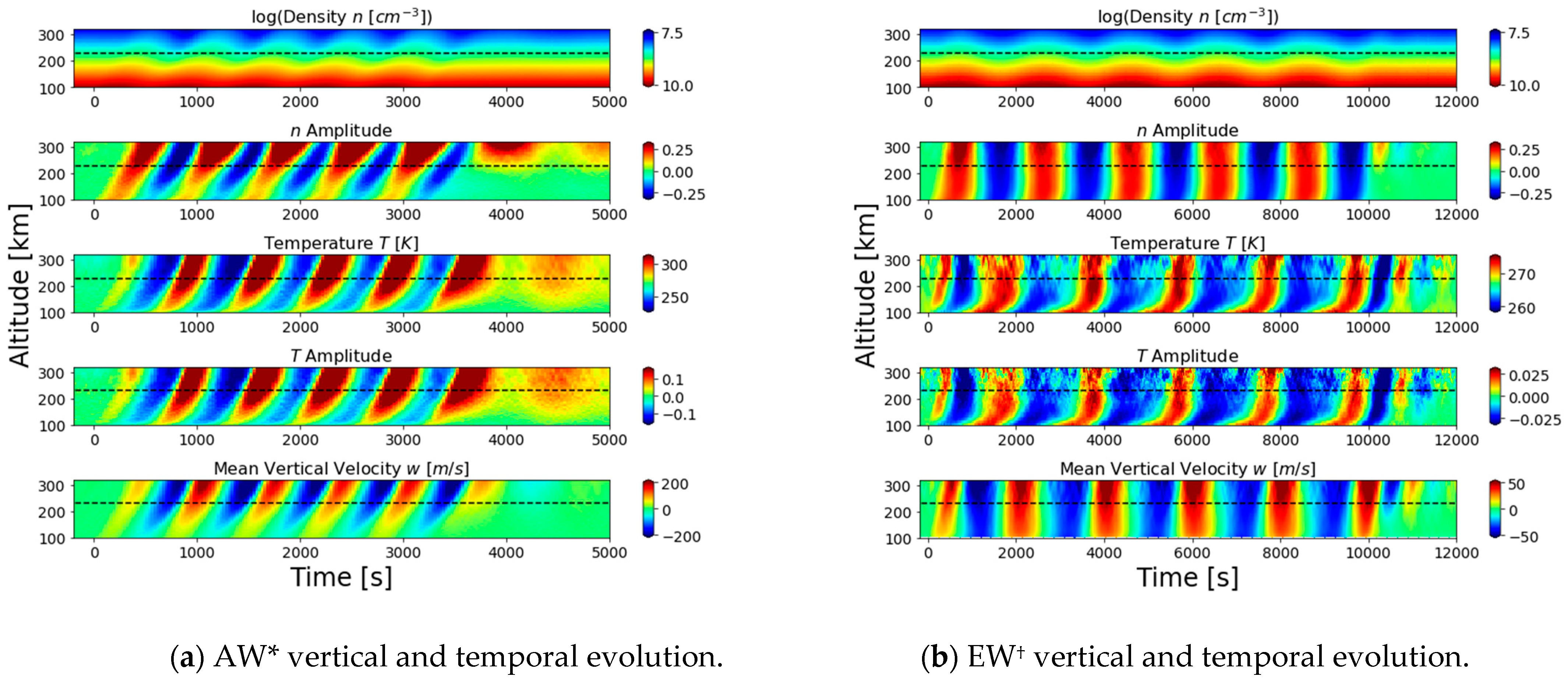
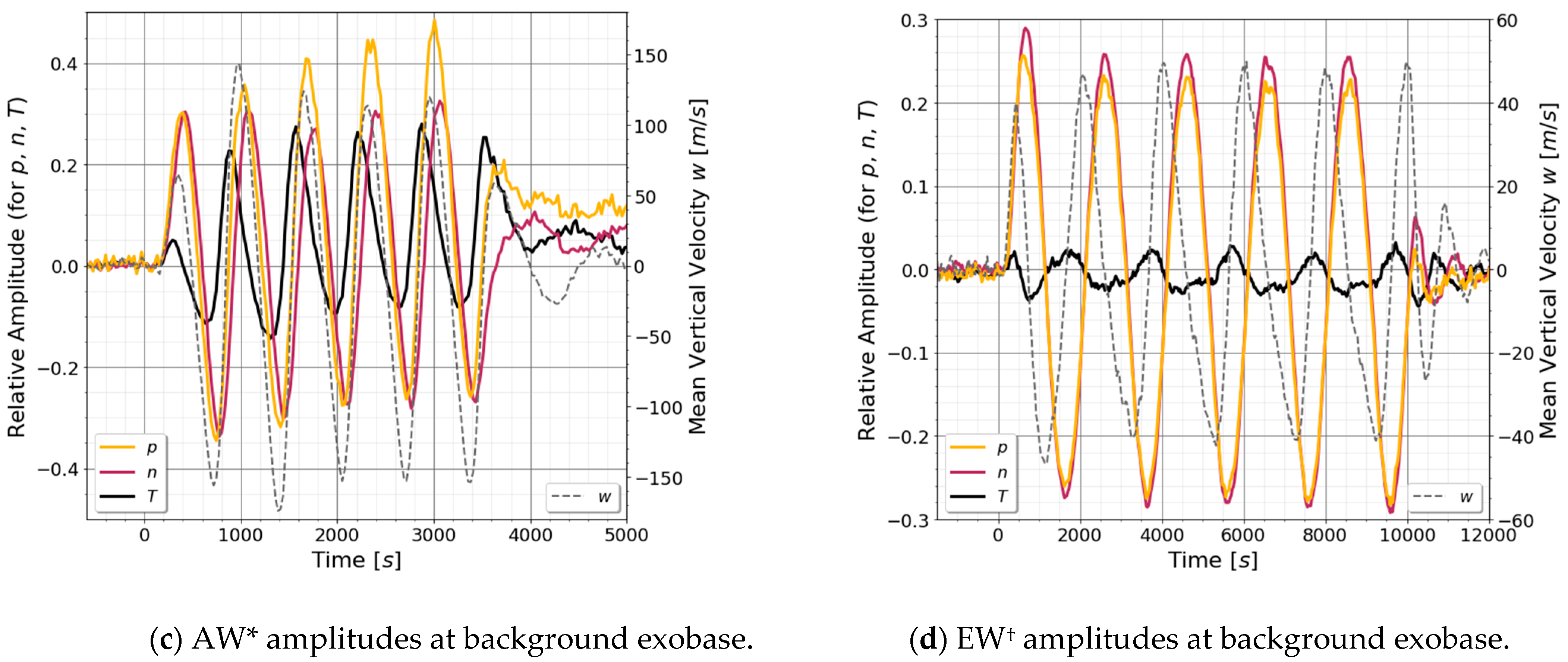
Figure 1 gives DSMC results showing the variation in the atmosphere properties vs. time and altitude produced by an AW (
Figure 1a,c) and an EW (
Figure 1b,d), Cases (*) and (
†) in
Table 1, respectively.
Figure 1a,b show that the vertical and transient behaviors for the two waves differ as expected. Whereas the density and temperature amplitudes of an AW grow significantly with altitude, as described quantitatively below, the EW amplitudes do not. The dashed horizontal lines mark the nominal exobase (230 km) for the initial background atmosphere.
Figure 1c,d exhibit the variability at the nominal exobase in the density, temperature, and pressure amplitudes (left axis), and the vertical flow velocity
(right axis) due to the onset of wave activity. The difference in phases between the density and temperature for the AW was found to have a similar dependence on the background parameters in the collisional regime as in the LAFM. However, as shown in L20, the extraction of temperature using only the density data, as often carried out using spacecraft density data, is problematic. For instance, the temperature amplitude is seen to be always smaller than the density amplitude, unlike what is sometimes found using density data along a spacecraft’s path. Results for simulations of other AWs with different background
and surface densities showed that the resulting oscillatory behavior and phase differences under steady wave activity were moderately affected by collisions, changing very roughly according to the parameters in the LAFM. On termination of the driving frequency after five periods, wave activity near the exobase, unsurprisingly, persisted for a number of cycles (
Figure 1c,d). Therefore, as is well understood, the typical interpretation of spacecraft density data can be problematic unless the activity is steady.
Figure 1.
AW and EW activity driven at the lower boundary as in Equation (1), with
as in Equation (2) and
for 5 periods after a steady-state isothermal atmosphere was achieved. Results: (
a,
c) Case (*) in
Table 1 with 200 cells; (
b,
d) Case (
†) in
Table 1 with 55 cells. In (
a,
b): amplitudes (color scales) vs. altitude and time: dashed lines indicate nominal exobase for background atmosphere. In (
c,
d): amplitudes vs. time at nominal background exobase (230 km): solid curves left axis, dotted right axis. Note: for the AW in (
c), net heating is indicated as the cycle-averaged temperature amplitude (red) is greater than zero; in (
d), fluctuations in the small temperature amplitude indicate the size of uncertainties.
For steady wave activity in the LAFM approximation (Equations (A3)–(A5)), the temperature/density amplitude ratio is:
for an AW and
for an EW, independent of altitude. For the cases in
Figure 1, these are 0.67 and 0.054, respectively, exhibiting a similar trend to approximate steady values in the simulations at the nominal background exobase, ~0.4 and ~0.1, with the differences due to the molecular nature of the simulations. For the AW in
Figure 1c, although the phases and the relative amplitudes differ from those in the LAFM, their variations with
are also similar. However, the temperature amplitude does not oscillate about zero at the nominal exobase. Rather, the cycle-averaged value is shifted upward, indicating, as expected, that net heating has occurred. Depending on the altitude, this added heat requires a number of cycles to dissipate after the wave activity ceases. Of course, heating does not occur in the LAFM, which is also the case for more elaborate linear models that include first-order viscosity and thermal conductivity terms (e.g., Equation (A5)). In those descriptions, heating is a second-order effect separately calculated using solutions to linear models, e.g., [
18,
19]. In MK simulations, however, it is a direct outcome as seen in
Figure 1c.
Figure 1b,d give the results for a 1D EW, and similar behavior is seen when simulations are carried out at the other background temperatures. Because of the longer period, the pressure and density amplitudes are similar in size and nearly in phase. The small temperature amplitude seen in
Figure 1d indicates that the gas is much closer to being equilibrated locally. Not only is the temperature amplitude a small fraction of the density amplitude, but the flow velocity and temperature are seen to be about
and
out of phase with the density amplitude, consistent with the LAFM in Equation (A5).
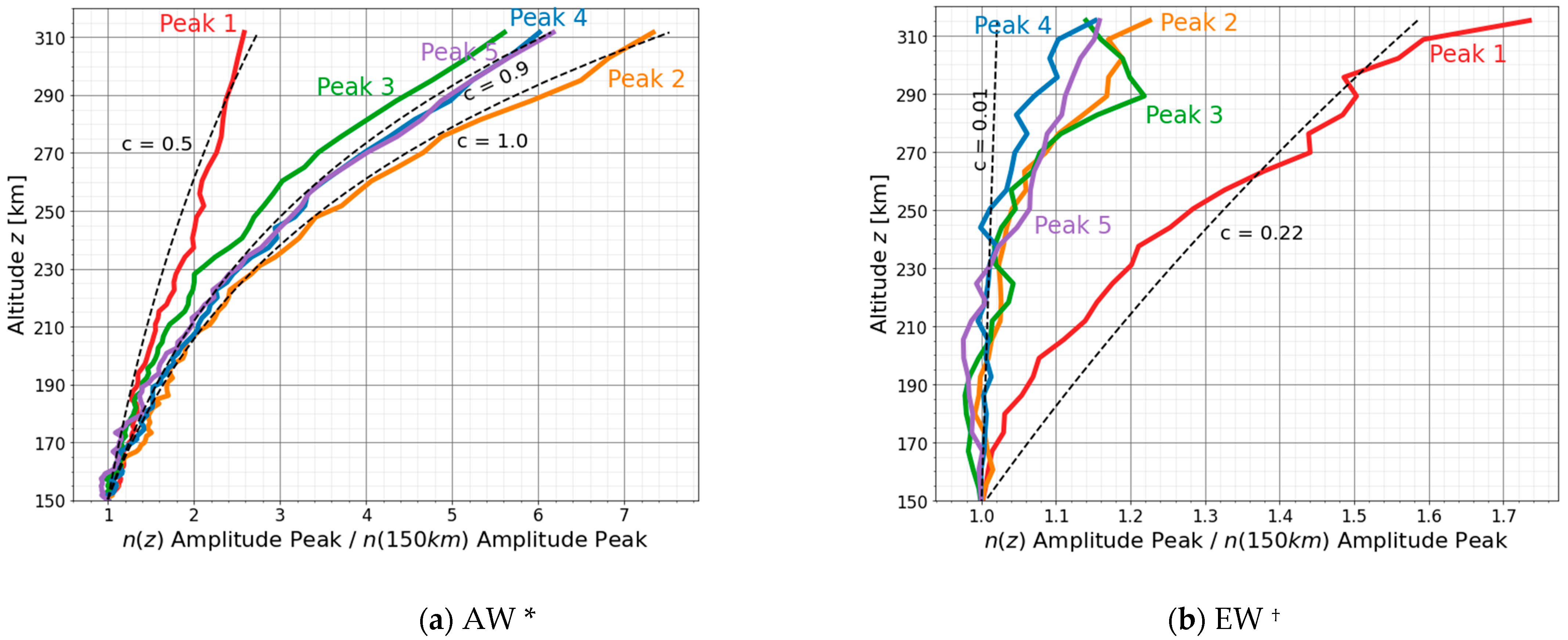
Figure 2a,b show the transient growth vs. altitude of the peaks in the density amplitude from 150 km to 300 km for the AW and EW simulations in
Figure 1. Each of the five density amplitude peaks across this altitude range is displayed as a ratio to the corresponding peak at ~150 km. As is well known, in the absence of viscosity and thermal conduction, the expected growth in the density amplitude of an AW is
, as seen in the
Appendix A. Therefore, dashed lines having the form
are drawn to guide the eye. The coefficient
, indicating the growth with altitude, is seen to vary in time as steady state is approached. Near steady state (Peak 5), the difference from
= 1 for the activity driven by an AW is, of course, due to the inclusion of molecular collisions accounting for the effect of viscosity and thermal conductivity. Therefore, the values of
for Peak 5 at the nominal exobase, written as
, are given in
Table 1, above. Results for simulations at other background temperatures were roughly consistent with those displayed.
For an initial isothermal atmosphere with scale height
, the AW amplitude in the LAFM grows exponentially with a scale height
(i.e.,
) as discussed above, whereas the amplitude for an EW is predicted to grow more slowly (i.e.,
), as shown in the
Appendix A. However, the simulation results in
Figure 2 indicate that, following the onset of wave activity, the transient amplitudes (the amplitudes of the sequential peaks), unsurprisingly, exhibit a very different behavior with altitude than the roughly steady wave values for both AW and EW. Therefore, in modeling wave activity, it is, again, clear that interpreting the density data vs. altitude along a spacecraft trajectory can be very problematic when the activity is variable.
Figure 2.
Growth in density amplitude peaks vs. altitude (km) divided by the respective density amplitude peak at 150 km, i.e.,
. Dashed lines of the form
are provided
as a guide, with
being the isothermal background scale height. (
a) Case (*) in
Table 1 (
in LAFM): 1st peak (
), 5th peak (
). (
b) Case (
†) in
Table 1 (
in LAFM): 1st peak (c~0.2) with rapid decay in the growth in the collisional regime, but slow decay above the nominal background exobase (230 km). Fluctuations indicative of uncertainties in peak positions.
Following the onset of wave activity for the AW Case (*) in
Table 1, above, the growth with altitude of the amplitude peaks in
Figure 2a approaches a rough steady state very differently than for the EW in
Figure 2b. Although the amplitude of the first pulse for an AW exhibits a growth with altitude much less than that predicted by the LAFM (
~0.5 vs.
),
increases to ~0.9 by the fifth peak as steady activity is approached, indicating that the effect of viscosity and thermal conductivity is not large. However, when doubling that frequency, we found that
is about 0.2 for the initial peak, whereas the result given in
Table 1 for the fifth peak is ~0.6. Therefore, the dissipative effect produced by simulating the molecular interactions is much larger at the higher frequency.
Following the onset for the EW case (
†) in
Table 1, the wave amplitude initially grows significantly with altitude. Although the initial growth with altitude is smaller, it is not unlike that of the initial AW peak. This is especially the case above the exobase, emphasizing the importance of understanding wave transients and variability. As the simulated EW approaches steady wave activity, the growth rapidly decays in the collisional regime, for which the LAFM predicts
. However, the perturbation in the exosphere is seen to approach a steady state value very slowly.
When
at the lower boundary (Case (
‡) in
Table 1, above), the scale factor
was again transient. It was ~0.4 at the first peak but in one period became ~0.7, very close to the
value given in
Table 1, above, but somewhat lower than the LAFM value
~0.8. Reducing
to 0.15, changing the temperature, or increasing the density at the lower boundary changed the magnitude, but not the trends, in these results.
The
values, also given in
Table 1 above, are estimates of
at the exobase for AWs calculated using Equation (A7). The expression in Equation (7) was derived from the linear fluid model given in Equation (A5) in the
Appendix A. This model includes, to first order, the viscosity and thermal conductivity, which are assumed to be small. It is seen that these values, evaluated at the nominal background exobase, exhibit a trend similar to the near-steady-state simulation results (
) shown for the AWs in
Table 1. This confirms that the collisional damping described in these simulations is consistent with fluid models and can affect the interpretation of observations of wave amplitude growth.
4. Heating
Since atmospheric temperatures are not directly measured by the Cassini or MAVEN spacecraft, the approximate temperature vs. altitude profiles on Titan and Mars are typically extracted from the 1D density data, e.g., [
1,
8]. The fact that the density and temperature peaks are out of phase, as seen in
Figure 1, suggests that this procedure might be problematic, as mentioned above. Earlier, we used a 2D LAFM model to show that, in the presence of wave activity, this extraction procedure is useful only over a limited range of wave parameters [
10]. L20 also used their 1D DSMC results to discuss this extraction method for atmospheres containing both one and two species. In the following, we discuss the heating seen in these simulations.
Consistent with the observation of reduced exponential growth of the density amplitude (i.e.,
Figure 2 and
in
Table 1 above), the implementation of molecular collisions also affects the temperature vs. altitude for an AW. Unlike in linear fluid models that include viscosity and thermal conduction, e.g., [
18], the effect on the temperature vs. altitude is a direct outcome of MK simulations, as also seen in
Figure 1c and
Figure 3a, and as mentioned earlier. That is, as an atmosphere is perturbed by the initiation of an acoustic wave,
gradually deviates from an oscillation about zero to an oscillation about a value that increases with time and with altitude, indicative of heating. For the case shown in
Figure 3a, the cycle-averaged shift in temperature,
, grows over the indicated altitude range from ~6 K to ~40 K. For those AWs simulated, we also found that the size of
increases nearly linearly with altitude in this region of the atmosphere. Column 5 in
Table 1 above gives an estimate of the near steady state, simulated, cycle-averaged change in temperature
over the background scale height in the exobase region. These values were estimated using the fifth perturbation cycle. While the AW cases exhibit significant heating, as expected, the EW for Case (†) exhibits very slight cooling. It is interesting, however, that when
at the lower boundary for Case (‡) in
Table 1, above,
begins to exceed the acoustic cutoff frequency as the altitude increases. Therefore, in the exobase regime, the cycle-averaged temperature
is seen to have increased significantly, similar to the AWs that have much higher frequencies at the lower boundary. The observed growth in the cycle-averaged temperature for thid case was also found to increase nearly linearly with altitude.
Figure 3.
For AW Case (*) in
Table 1, temperature and density amplitudes vs. time (as in
Figure 1c) at a number of altitudes: (
a)
, and (
b)
. The cycle-averaged density above the nominal background exobase is seen to increase significantly.
Figure 3.
For AW Case (*) in
Table 1, temperature and density amplitudes vs. time (as in
Figure 1c) at a number of altitudes: (
a)
, and (
b)
. The cycle-averaged density above the nominal background exobase is seen to increase significantly.
For the amplitudes used here, such increases in
do not cause significant Jeans escape of O but can affect the escape of the often concomitant, lighter species H
2, as well as affect the local atmospheric chemistry. However,
Figure 3b shows that the increase in
with altitude can significantly affect the density amplitude above the nominal background exobase, a process suggested by MAVEN data [
2,
5]. Below the nominal background exobase in these simulations (~230 km), the density amplitudes are close to LAFM predictions, as in
Figure 1c. However, above the exobase, the cycle-averaged heating has a significant effect on not only the density amplitude but also the cycle-averaged density (~20%) as steady activity is approached. Such an increase can affect the interaction of the molecules driven into the corona by wave activity with the ambient space plasma. These interactions are a principal driver of escape on Mars and Titan, e.g., [
1,
20]. This increase is often suppressed in fluid models by the assumed upper boundary conditions, but is a natural outcome of the MK simulations. Of course, in 2D, the variable and enhanced perturbations above the nominal exobase can eventually be dispersed by ballistic transport and wave saturation, e.g., [
5]. However, our simulations also show how the perturbations propagating into the coronal region dissipate only slowly after the wave activity at the lower boundary ceases. This can significantly alter the interpretation of spacecraft data when fluid models for steady wave activity are used to fit the data, which is often the case.
The temperature increases in
Table 1 for AWs, as well as those calculated for
and other background temperatures and densities at the lower boundary, were found to roughly scale with amplitude squared and with
when
. In these simulations, heating is primarily due to the forcing of the gas in a gravitational field, and the net cooling during steady activity is primarily due to the downward flow across the lower boundary. Whereas low-frequency waves can approach nearly adiabatic transport, the much more rapid forcing by the AWs causes compression and mixing of gas with different temperatures and densities vs. altitude. In fluid models, those heating effects are described by a number of second-order terms in the heat equation, with the dominant contribution for the parameters here being the divergence of the sensible heat flux [
19].
5. Summary
We expanded here on the results presented in Leclercq et al. [
13] in order to demonstrate the usefulness of molecular kinetic (MK) simulations for describing the effect of wave activity in the rarefied region of a planetary atmosphere. Such simulations are essentially equivalent to solving the Boltzmann equation [
15,
21]. The significant and variable wave activity observed in the exobase regions of Titan and Mars, which is of considerable interest, e.g., [
2,
7], does not appear to significantly affect the thermal escape of the dominant constituents, e.g., [
7,
8]. However, we show that such activity does affect the population and extent of the atmospheric corona, which in turn determines its interaction with the space environment.
Below the exobase and near steady activity, the resulting density amplitudes are shown to be roughly consistent with those predicted by 1D steady wave activity models in the
Appendix A. Allowing for conditions that are typically applied at the lower boundary, any differences in the phases and amplitudes are, of course, due to the direct inclusion of molecular collisions. However, in the region from which escape can occur, these simulations exhibit significant differences from fluid models. In addition, as discussed above, the temperature profiles are a direct outcome of the simulations, which were seen to increase nearly linearly with altitude for AWs propagating to the exobase. These 1D results, therefore, indicate that molecular simulations are needed to improve our understanding of the effect of gravity waves driven from below on the exobase region and on the content of the extended corona of a planet’s atmosphere. These are regions of the atmospheres on planetary bodies often studied by spacecraft in situ, or by remote sensing of auroral activity, but often not accurately modeled using fluid dynamics.
The results presented also show the importance of understanding the transient behavior in a highly variable atmosphere by simulating the onset and decay of wave activity in a thin atmosphere driven from below. Such variability can also be introduced by a transient heat pulse in the thermosphere driven externally by solar activity or by the ambient plasma, as considered in L20. Although we examined a range of amplitudes at the lower boundary, as suggested by observations in the upper atmosphere of Mars, e.g., [
2,
5,
22], for emphasis, we primarily presented results for a flux amplitude at the lower boundary of 0.25, our largest value for which escape is still negligible. As described, this corresponds to a significant but realistic density amplitude at the lower boundary of ~0.16 [
2,
3].
Figure 1 and
Figure 3 show that the transient wave activity persists in the extended corona for a number of cycles beyond the termination of wave activity at depth. When using only density observations of waves vs. altitude, this can affect the interpretation of wave type and, therefore, the estimates of the net heating.
Figure 2 also shows that, near the onset of wave activity, it can also be difficult to separate an EW disturbance from an AW disturbance without additional information on the horizontal structure or frequency of the perturbation. Such data is often not available from in situ spacecraft measurements. Finally, MK simulations are useful as they also directly determine the nonlinear effects on the amplitudes and phases in the rarefied region, as well as on the heating vs. altitude, a principal goal of the considerable literature on wave activity, e.g., [
8].
Although it is unlikely that highly perturbed upper atmospheres can be described as having an isothermal background, or that the activity can be approximated using steady-state models in a highly variable atmosphere such as that on Mars, such assumptions are often made. However, it is clear that transients and atmospheric variability can be readily incorporated into MK simulations when describing the propagation of wave energy into the region of a planetary atmosphere that transitions from collision-dominated to a nearly collisionless corona.
Of course, when wave activity occurs over many scale heights, an MK model would need to be coupled to a fluid model from below for computational efficiency [
23]. Although the background gravity, temperature, and density used are Mars-like, consistent with L20, the vertical wavelengths initiated are relatively long in our simple O upper atmosphere. Therefore, this work is intended to show the effects revealed by using a molecular model to describe the propagation of wave energy into the exobase regime. Of course, wave activity in a real atmosphere requires multi-dimensional, multi-component MK simulations, which are now underway.


 ,
, 


