A Hybrid Deep Learning Model for Air Quality Prediction Based on the Time–Frequency Domain Relationship

Abstract

Deep learning models have been widely used in time-series numerical prediction of atmospheric environmental quality. The fundamental feature of this application is to discover the correlation between influencing factors and target parameters through a deep network structure. These relationships in original data are affected by several different frequency factors. If the deep network is adopted without guidance, these correlations may be masked by entangled multifrequency data, which will cause the problem of insufficient correlation feature extraction and difficult model interpretation. Because the wavelet transform has the ability to separate these entangled multifrequency data, and these correlations can be extracted by deep learning methods, a hybrid model combining wavelet transform and transformer-like (WTformer) was designed to extract time–frequency domain features and prediction of air quality. The 2018–2021 hourly data in Guilin was used as the benchmark training dataset. Pollutants and meteorological variables in the local dataset are decomposed into five frequency bands by wavelet. The analysis of the WTformer model showed that particulate matter (PM_2.5 and PM₁₀) had an obvious correlation in the low-frequency band and a low correlation in the high-frequency band. PM_2.5 and temperature had a negative correlation in the high-frequency band and an obvious positive correlation in the low-frequency band. PM_2.5 and wind speed had a low correlation in the high-frequency band and an obvious negative correlation in the low-frequency band. These results showed that the laws of variables in the time–frequency domain could be found by the model, which made it possible to explain the model. The experimental results show that the prediction performance of the established model was better than that of multilayer perceptron (MLP), one-dimensional convolutional neural network (1D-CNN), gate recurrent unit (GRU), long short-term memory (LSTM) and Transformer, in all time steps (1, 4, 8, 24 and 48 h).

1. Introduction

Over the past few decades, with the continuous advancement of industrialization and urbanization, the huge consumption of energy has led to the increasingly serious problem of air pollution [1,2,3]. Air pollutants include PM_2.5, CO, SO₂, NO₂, etc., which can cause many diseases, such as asthma, heart disease, chronic obstructive pulmonary disease and cancer [4,5]. According to the World Health Organization (WHO), simple breathing behavior causes 7 million deaths each year due to air pollution, which seriously endangers human health. To reduce the harm caused by air pollution, researchers have introduced various models to predict changes in air pollution to take necessary measures at the corresponding time [6,7]. Among these models, the deep learning model has the best prediction effect [8]. However, the deep learning models have the “black box” problem, and the prediction behavior of the models is difficult to explain. In addition, the time-series data of the atmospheric environment integrates signals of different frequencies and is mixed with incorrect noise signals, the correlation between atmospheric and pollutant variables is masked by these entangled signals, so it is difficult to be reliably found. Therefore, it is very important to improve the interpretability and accuracy of the prediction by separating the entangled different frequency signals from the original data to obtain clearer signals and designing an interpretable network to extract these correlation rules.

Thus far, various technical methods have been applied to air quality prediction, including mechanism models and statistical models. The mechanism models were established by simulating physical and chemical processes of air diffusion, such as Gaussian diffusion models [9,10], weather research and forecasting (WRF) models [11,12,13] and community multiscale air quality (CMAQ) models [14,15]. For example, Cheng et al. proposed an inference model based on the Gaussian process to estimate the pollutant concentration at any point [16]. Rogers et al. established the WRF model configuration through various sensitivity experiments in central California, allowing WRF to simulate meteorological variables with reasonable errors [17]. Lee et al. analyzed and evaluated atmospheric O₃ using a CMAQ modeling system to help air pollution control in China [18]. However, detailed and accurate external environmental parameters were required as inputs to the mechanism model. Owing to the complexity of real environment, these parameters were difficult to obtain reliably, which makes prediction of the mechanism models have great limitations. Statistical models were used to predict future changes in variables by discovering the evolution of data from historical data, including linear regression models [19,20], perceptron [21,22], support vector machine (SVM) [23,24], tree models [25,26,27], deep neural networks (DNN) [28,29,30], etc. Linear regression models include univariate linear regression and multivariate linear regression; between them, multivariate linear regression had better nonlinear fitting ability, but it may be insufficient compared with perceptron, tree models, DNN, etc.

With the continuous development of artificial intelligence technology, new models of DNN have been continuously constructed and improved, such as convolutional neural networks (CNN) [31], graph convolution networks (GCN) [32], LSTM [33], residual networks (ResNet) [34], attention network [35] and Transformer [36], which have been widely used in air pollution prediction. At the same time, the huge improvement in graphics processing unit (GPU) computing power makes it possible for complex DNN models to be trained, the prediction performance of DNN has been superior to other traditional statistical models [37], which may be explained by two reasons. First, the deep network structure gives it stronger ability to simulate the evolution process from input to output. Second, various network modules were flexibly combined, and the advantages of various networks were utilized. For example, a deep distributed fusion network was constructed based on deep neural networks [38], which had been improved for both short-term and long-term prediction of air quality compared to previous online monitoring systems. A deep convolutional neural network was used to correct the prediction error of CMAQ, which improves the prediction performance of the CMAQ model [39]. CNN-LSTM and GCN-LSTM combined the advantages of CNN/GCN to extract spatial information and LSTM to capture time dependence, showing advanced prediction performance [40,41]. However, the deep network structure makes the prediction of the model difficult to explain, and the prediction behavior of the models is difficult to understand, which is not conducive to taking corresponding measures to alleviate air pollution. Moreover, the complex and changeable atmospheric environment makes the air pollutant data integrate entangled signals of different frequencies, accompanied by various incorrect random noise, which affects the accuracy of prediction.

To overcome these limitations, we designed a hybrid model based on wavelet transform, attention network and LSTM to predict the changes in air pollutants. The developed model has the following innovations: (a) The frequency separator was constructed by wavelet transform, which separates the entangled different frequency data in the original data, so that the correlation between pollutants and meteorological variables is clearer and the prediction accuracy is improved. (b) The self-attention network was improved to better discover the time–frequency correlation between pollutants and meteorological variables, and the focus of the model is found by analyzing the attention matrix, so that the prediction behavior of the model can be explained. (c) An intelligent model combining deep learning and time–frequency correlation extraction was established to reflect the deeper time–frequency relationship between pollutants and meteorological variables in the study area.

The structure of the paper is as follows. In Section 2, the principles and functions of the techniques used in the model and the sources of research data are introduced. Section 3 introduces the structure of the model. Section 4 evaluates the predictive performance, interpretability and necessity of each module in the model. Section 5 summarizes this work and looks forward to the future direction.

2. Problem Scenario

In the study, PM_2.5 was used as the target parameter, other pollutants and meteorological parameters as the impact parameters, including PM₁₀, CO, wind speed, temperature, humidity, etc., and there is a correlation between them [42]. Meteorological and pollutant data are typical time-series data. Because of the complexity of the real environment, the time-series data were affected by factors of different frequencies, and the time-series data were mixed with signals of different frequencies.

The entangled signals of different frequencies in the original data can be separated by wavelet transform, which is beneficial when trying to locate the time correlation between variables more accurately. Self-attention can be used to construct the feature encoder, calculate the correlation matrix between different frequency bands of meteorological and pollutant variables, and enhance the data characteristics of the main influencing factors, which is conducive to improving the prediction accuracy. By analyzing the correlation matrix among different frequency bands of each variable, the main factors effecting the short-term mutation and long-term trend of the prediction target can be found, which improved the interpretability of the model. The decoder’s decoding process, LSTM, was used to decode time information and capture time dependencies and the attention network was used to adaptively extract primary features from time-decoded data to predict PM_2.5 concentrations.

The WTformer model combines the advantages of wavelet transform and deep learning methods, which effectively improves the interpretability and prediction accuracy of the model.

2.1. Wavelet Transform Used for Time-Series Decomposition

Wavelet transform is a mathematical tool used to separate different frequency information from original data by adaptively exploring different frequency bands through a wavelet mother function [43]. This method can overcome the shortcomings of the short-time Fourier transform, which is difficult to analyze time-varying signals effectively [44]; it is an effective tool for processing and analyzing time-series data of air pollution [45,46,47]. Wavelet transform can be defined as follows:

$$WT\left(a,b\right)=\frac{1}{\sqrt{a}}{\int }_{-\infty }^{\infty }f\left(t\right)\psi \left(\frac{t-b}{a}\right)d_t,$$

(1)

where $\frac{1}{\sqrt{a}}$ is the normalization factor, $f\left(t\right)$ is the input signal, $\psi \left(t\right)$ is the mother wavelet, $a$ is the scaling exponent parameter and $b$ is the time-shifting parameter.

In this study, we used the stationary wavelet transform (SWT). Its decomposition process includes translation invariance, which is conducive to the exploration of laws and the calculation of tensors. SWT divides the time-series data into high-frequency and low-frequency signals. High-frequency signals represent the short-term mutation characteristics of the sequence, and low-frequency signals represent the long-term trend characteristics of the sequence [48]. In the SWT, we used the Daubechies (db) wavelet, which is the most commonly used wavelet [47], as the mother wavelet function.

2.2. Encoder

The encoder calculates the correlation between different frequency bands of input variables through self-attention to enhance the input feature information. The ability of self-attention to adaptively learn the correlation between input variables has played a crucial role in time-series prediction [49,50,51]. This structure is shown in Figure 1a. The calculation process of self-attention can be summarized as mapping input V to output by calculating the correlation matrix between variables. First, the input variables are mapped to different spaces using different linear layers, resulting in Q, K and V. Second, use all K to calculate the dot product of Q. Then, to prevent the activation function from being pushed to the minimum gradient region due to the dot product being too large, divide each by $\sqrt{d_k}$, and the correlation coefficient between the variables can be obtained. Third, by using the activation function SoftMax, the correlation coefficient can be mapped to (0, 1) to obtain a correlation matrix among the variables. Finally, the correlation matrix and V dot products are used to enhance the characteristic information of the data, that is, the variables associated with PM_2.5, which are greater after enhancement by the correlation matrix. Self-attention can be described in mathematical language as follows:

$$Attention\left(Q,K,V\right)=softmax\left(\frac{Q{K}^T}{\sqrt{d_k}}\right)V,$$

(2)

where Q represents the information to the query, K represents the key to the query and V represents the value of the query.

In the original self-attention, V was mapped to another vector space by the linear layer, which may have caused the information of the original space to be destroyed and the correlation among variables to be blurred, which was not conducive to the interpretation of the model. In addition, in Scaled Dot-Product Attention, SoftMax was used as the activation function, and its range was limited to (0, 1), which confused negative and weak correlations when calculating correlations among variables. To solve these problems, the linear layer on V was canceled, and we used the Tanh activation function with a range (−1, 1) instead of SoftMax. The new self-attention structure is shown in Figure 1b.

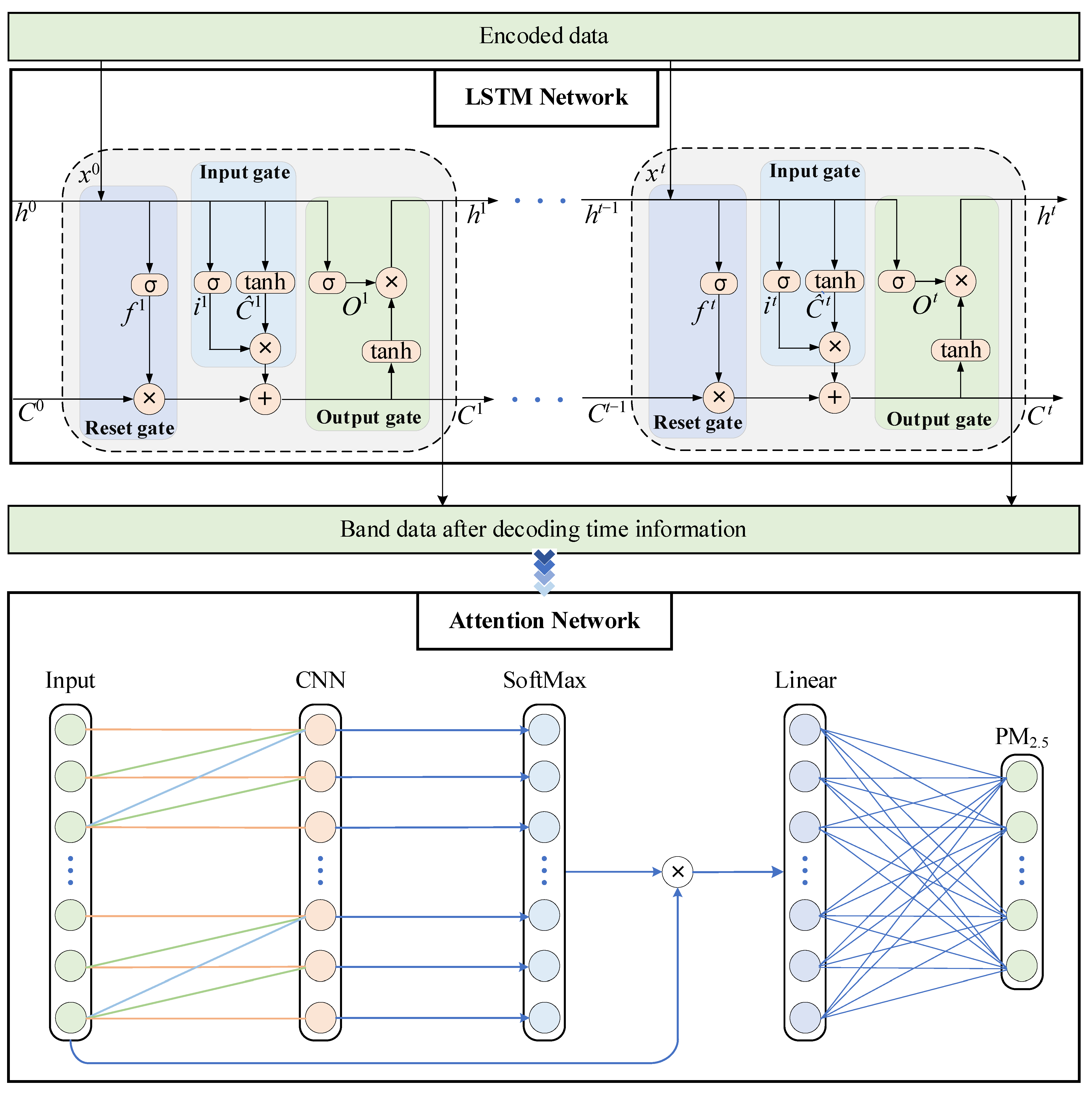
2.3. Decoder

In the decoding process of the decoder, LSTM was used to decode time information and capture time dependence, and the attention network was used to adaptively extract the main features from the time-decoded data to predict PM_2.5 concentration.

2.3.1. LSTM

LSTM is a gated deep learning network for time-series prediction. In the decoder, it was used to extract the time dependence between variables. Its structure is shown in Figure 2.

Each LSTM neuron has three gating units, which are the input gate, forgetting gate and output gate. By using LSTM internal gates, the time dependence on data can be resolved. The calculation of the LSTM unit is as follows:

$$f_t=\sigma \left(W_f\left[x_t, h_{t-1}\right]+b_f\right),$$

(3)

$$i_t=\sigma \left(W_i\left[x_t, h_{t-1}\right]+b_i\right),$$

(4)

$$O_t=\sigma \left(W_O\left[x_t, h_{t-1}\right]+b_O\right),$$

(5)

$${\widehat{C}}_t=\tanh \left(W_C\left[x_t,h_{t-1}\right]+b_C\right),$$

(6)

$$C_t=f_t·C_{t-1}+i_t·{\widehat{C}}_t,$$

(7)

$$h_t=O_t·\tanh \left(C_t\right),$$

(8)

where $W_f$, $W_i$, $W_O$ and $W_C$ are weight matrices; $b_f$, $b_i$, $b_O$ and $b_C$ are bias constants; and $\sigma$ is the corresponding sigmoid function. The neural network filters the data through the forgetting gate $f_t$. By evaluating the forgetting information of the previous state $f_t·C_{t-1}$, the useful information $i_t·{\widehat{C}}_t$ is remembered from the current state, and then $h_t$ is fed forward to the next hidden LSTM layer to update the state $C_t$.

2.3.2. Attention

In the decoder, the attention network was used to intelligently extract effective information from data at different time points. Attention has the effect of improving the accuracy and stability of model prediction and has been widely used in time-series prediction [52,53,54]. The attention function can be described as mapping the input $x$ to the output $y$ through the correlation matrix, and the correlation matrix was learned by the neural network. This process can be described in mathematical language as follows:

$$y=\alpha \left(x\right)·x,$$

(9)

where $\alpha$ is a neural network with $x$ as input, $\alpha \left(x\right)$ is the correlation matrix learned by the network, $x$ is input and $y$ is output.

The attention mechanism is different from Q-K-V self-attention. In terms of computational complexity, the time complexity was O(n), and compared with the square complexity of the self-attention module, the attention model was faster. Functionally, although attention could not find the correlation between input variables, it could intelligently discover and extract effective information from redundant information through the network. Thus, it could reduce the computational complexity while also ensuring the model prediction performance.

2.4. Data Sources

The study area is located in Guilin, China, shown geographically in Figure 3a. The research data are from online atmospheric monitoring stations in Guilin, including 10 fixed stations and 51 micromonitoring stations. The fixed stations include Dianzikeda, Luyouxueyuan, Chuangyedasha, Bazhong, Linchuan, Linkesuo, etc. The microstations include Wanfulu, Lijiangdamei, Jiangjunluxi, Xinxichanyeyuan, Shahelijiao, Hongjie, etc. Figure 3b shows the geographical distribution of these stations. The average hourly data from 2018 to 2021 for meteorological variables and pollutant concentrations were used as the basic dataset.

Table 1. Pollutants and meteorological variables in the dataset.

Categories	Variables	Unit
Pollutant	PM2.5	ug/m3
	PM10	ug/m3
	CO	ug/m3
	NO2	ug/m3
	SO2	ug/m3
	O3	ug/m3
Climate variables	Wind speed	m/s
	Temperature	°C
	Humidity	%
	Rain	mm
	Pressure	hpa

lists the pollutants and meteorological variables in the basic dataset. The meteorological variables include wind speed, temperature, humidity, air pressure and rainfall. The pollutant variables include PM_2.5, PM₁₀, NO₂, CO, SO₂ and O₃. PM_2.5 in the sample area was used as the prediction target for the model.

Guilin is a famous tourist city, attaching great importance to the protection of the ecological environment, with magnificent mountains and clear rivers. However, the air quality index is the worst among the 14 cities in Guangxi Province, and haze events often occur in winter [55]. This abnormal phenomenon is due to the special geographical location. As shown in Figure 4, the area northeast of Guilin is connected to Yongzhou through Lingchuan, Xing’an and Quanzhou, and the area southwest is connected to Liuzhou through Yongfu. In addition, Guilin is a typical karst basin, surrounded by Tianping, Haiyang, Jiaqiao and other mountains, which readily forms atmospheric turbulence and is not conducive to the diffusion of atmospheric pollutants. Therefore, the pollutants from Yongzhou and Liuzhou often accumulate in Guilin, resulting in abnormal haze events in Guilin, so it is necessary to make a reliable prediction of air pollutants in Guilin.

Atmospheric turbulence in Guilin varies greatly in different seasons and periods, resulting in obvious high- and low-frequency fluctuations. It is characterized by the large influence of exogenous long-distance transport in autumn and winter, and the large influence of local turbulence in spring and summer. Therefore, sample data from this region are suitable as the basic data for the model.

3. Methods

3.1. Framework

In this study, we constructed a hybrid prediction model combining wavelet transform and deep learning. The model framework is shown in Figure 5. The framework included data acquisition and processing, frequency separation, WTformer, result analysis and correlation analysis. First, hourly air pollutants and meteorological data were collected and preprocessed. Second, the low-frequency and high-frequency signals were separated from the original data by the frequency divider. Third, the WTformer model was constructed to predict future changes in PM_2.5 concentration. Fourth, root mean square error (RMSE), mean absolute error (MAE) and symmetric mean absolute percentage error (SMAPE) were used as evaluation parameters. The WTformer was compared with the established baseline model and ablation model to verify the prediction performance. Finally, the correlation matrix learned by the model was analyzed to obtain the deeper time–frequency law of the meteorological and environmental variables.

3.2. Data Processing

Deep learning models are based on statistics, which predict the future evolution of variables by mining rules from data, so reliable data are needed as input. However, monitoring data often appear abnormal because of instrument failure, network loss, abnormal weather, power failure and other reasons. The processing of outliers includes two cases: missing values were filled by linear interpolation, and the $3\sigma$ method was used to identify outliers and fill them by linear interpolation. In addition, data of the same magnitude are used as input to the deep learning model, which helps to smooth the learning gradient, thus improving the accuracy and stability of the prediction; therefore, the data of meteorological and pollutant variables need to be normalized. Min–max normalization was used in the paper, as shown in Equation (10).

$$x^{\prime }=\frac{x-x_{min}}{x_{max}-x_{min}}$$

(10)

where $x^{\prime }$ is the normalized value, $x$ is the original value, $x_{min}$ is the minimum value in the data and $x_{max}$ is the maximum value in the data.

3.3. Construction of Frequency Separator

We built the frequency splitter using SWT, which was designed to separate low- and high-frequency signals in pollutants and meteorological parameters. Its structure is shown in Figure 6. The timing diagram of Figure 6 was obtained by decomposing 512 h of PM_2.5 data.

First, the original time-series data were decomposed into low-frequency component CA₁ and high-frequency component CD₁ by SWT. Because the decomposition process of SWT did not extract coefficients at each transform level, CA₁ and CD₁ had the same dimension as the original data. Then, CA₁ was decomposed in the same way to obtain CA₂ and CD₂. The low-frequency component CA_n and the high-frequency component CD_n were obtained by recursive calculation, where n represents the decomposition scale. The larger the number of decomposition layers, the more detailed information was lost in the low-frequency signal. The number of decomposition layers used in this study was four.

3.4. Construction of Encoder

The encoder was constructed by improving self-attention. It was used to calculate the correlation matrix between meteorological and pollutant variables, to enhance feature information and to encode. Its structure is shown in Figure 7.

First, Q and K were obtained to map the time–frequency data of meteorology and pollutants to different spaces through the linear layer. Then, the transpose matrix of Q and K was multiplied to calculate the correlation coefficient between variables and the correlation matrix was obtained by using the Tanh activation function after normalization. Finally, the correlation matrix was multiplied by the input original data V matrix to enhance the feature information for the data. The more variables associated with PM_2.5, the greater its value would be after feature enhancement, thereby enhancing the feature information for the main influencing factors and reducing the impact of interference signals.

3.5. Construction of the Decoder

The decoder was constructed by the LSTM and Attention modules. It was used to decode the time information and extracted valid feature information from the time step to predict future PM_2.5 concentrations. Its structure is shown in Figure 8.

First, LSTM was used to decode time information in the time dimension to capture time dependencies. Second, the time-decoded data were input into the Attention Network, and the convolutional layer was used to extract the variable information in each frequency band and the feature bands of the correlation between PM_2.5 and meteorological and pollutant parameters in different frequency bands. Third, the SoftMax layer was input to obtain the correlation matrix of each frequency domain for the prediction results. Fourth, the correlation matrix was multiplied by the data after time decoding to enhance the feature information for the main frequency bands. Finally, the PM_2.5 concentration in the future was predicted by fusing the feature information with the linear layer.

3.6. Evaluation Criterion

To quantify the predictive performance of the model, RMSE, MAE and SMAPE were used as evaluation indexes:

$$MA{E}_{\left(y^{\prime },y\right)}=\frac{1}{n}{\displaystyle \sum }_{i=1}^n\left|y_i^{\prime }-y_i\right|,$$

(11)

$$RMS{E}_{\left(y^{\prime },y\right)}=\sqrt{\frac{1}{n}{\displaystyle \sum }_{i=1}^n{\left(y_i^{\prime }-y_i\right)}^2},$$

(12)

$$SMAP{E}_{\left(y^{\prime },y\right)}=\frac{1}{n}{\displaystyle \sum }_{i=1}^n\frac{\left|y_i^{\prime }-y_i\right|}{\frac{y_i^{\prime }+y_i}{2}},$$

(13)

where n is the total number of samples, $y_i^{\prime }$ is the predicted value and $y_i$ is the observed value.

4. Experimental Results and Analysis

4.1. Network Parameters

The small-batch gradient descent algorithm was used to optimize the model. The size of each batch was 32, and the training was repeated for 200 rounds. When the loss value of the training dataset does not decrease within five rounds, the early stop method was used to stop the training. The dropout of 0.1 was set to prevent overfitting. Additionally, a number of hyperparameters were debugged to anticipate that the model achieved the best performance, including historical time step, wavelet decomposition scale, linear mapping layer dimension, etc., where the historical time step represents the length of the historical time unit used to predict future data, the wavelet decomposition scale represents the number of rounds of the original data being decomposed by wavelet, and the linear mapping layer dimension represents the dimension of the data being mapped to the hidden space.

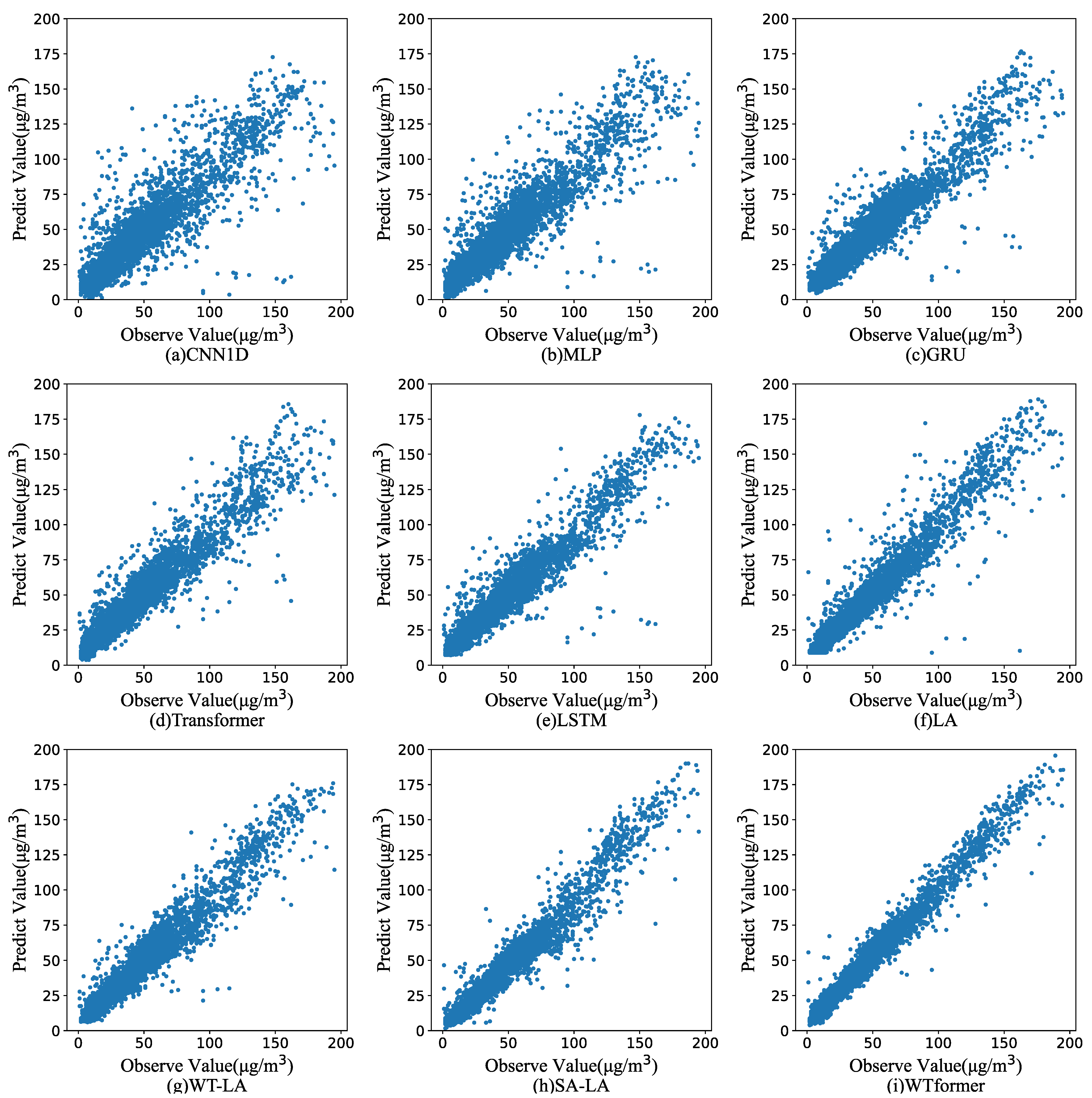
4.2. Prediction Performance

To evaluate the predictive performance of WTformer, the air pollutant concentration from January 2018 to January 2021 was used as the learning data, and the average hourly PM_2.5 concentration of the two periods was used as the test data to evaluate the performance of WTformer in different situations. During the period from 7 to 23 May 2021, the change in PM_2.5 concentration showed a normal trend. From 1 July to 16 July 2021, PM_2.5 concentration changes frequently. Figure 9 and Figure 10 show the prediction structure of WTformer in two time periods. In different situations, the model showed good prediction performance.

4.3. Ablation Experiment

The ablation model was established by removing some modules in the hybrid model. Its experimental purpose was to ensure that the introduction of each module in the model was effective for improving the prediction accuracy. Self-Attention LSTM Attention (SA-LA), Wavelet Transform LSTM Attention (WT-LA) and LSTM-Attention (LA) were constructed for ablation experiments. Among them, the SA-LA was constructed by removing the wavelet decomposition module, the WT-LA was constructed by removing the feature enhancement module, and the LA model was constructed by removing the wavelet decomposition and feature enhancement modules. With the same number of training rounds and learning rate, the concentration of PM_2.5 in the next 48 h was predicted by WTformer and the three ablation models. The predicted and observed values are shown in Figure 11. By analyzing the performance of each model at markers 1, 2, 3, 4, it can be found that the WTformer model performs best, whereas the SA-LA and LA models, which lacked the wavelet decomposition module, were less sensitive to the mutation. The WT-LA and LA models, which lacked the feature enhancement encoder, had a prediction lag problem at markers 1 and 3.

These ablation experiments verified that each module in the WTformer model was effective. The wavelet decomposition module improved the sensitivity of the model to mutation. The feature enhancement module alleviated the lag problem of the LSTM model in prediction.

4.4. Correlation Analysis between PM_2.5 and Other Variables

We conducted a correlation analysis to determine the influence of meteorological and pollutant parameters on PM_2.5 at a deeper level to show the interpretability of the model. To analyze the factors affecting the variation in PM_2.5 for different frequency bands, Figure 12 shows the attention matrix learned by self-attention in the encoder. Among the pollutant factors, the correlation between PM_2.5 and PM₁₀/NO₂/CO/SO₂ was reflected mainly in the low-frequency band and slower frequency band in the high-frequency band, and the correlation was lower in the high-frequency band. The correlation between PM_2.5 and O₃ was reflected mainly in the slower high-frequency band, and the correlation was lower in the low-frequency band and the faster high-frequency band. Among meteorological factors, the correlation between PM_2.5 and temperature/wind speed/pressure/precipitation were reflected mainly in the low-frequency band, and the correlation was weak in the high-frequency band. The correlation between PM_2.5 and humidity was reflected mainly in the slower high-frequency band, and the correlation was weak in the low-frequency band.

These findings indicated that the influence of PM₁₀/NO₂/CO/SO₂/temperature/wind speed/pressure/precipitation on PM_2.5 was reflected mainly in a wider time scale, and the influence was long term, whereas the influence of O₃ and humidity on PM_2.5 was reflected mainly in the high-frequency band, and the influence was short term. This shows that the time–frequency law between variables was found, and the prediction behavior of the model could be explained by analyzing the attention matrix.

4.5. Comparison of WTformer with Other Methods

To validate the advanced predictive performance of the WTformer model, it was quantitatively compared with the predictive performance of the ablation model and the mainstream deep learning models at different time steps (1, 4, 8, 24 and 48 h). The deep learning models include MLP, CNN1D, GRU, Transformer and LSTM.

Table 2. Comparison of model performance.

		MLP	CNN1D	GRU	Transformer	LSTM	LA	WT-LA	SA-LA	WTformer
+1 h	RMSE	7.475	7.349	6.799	8.083	6.840	6.614	6.475	6.404	6.334
	MAE	4.406	3.815	3.567	4.117	3.270	3.146	3.061	3.034	3.002
	SMAPE	0.119	0.106	0.086	0.117	0.084	0.081	0.080	0.077	0.076
+4 h	RMSE	15.554	16.364	13.099	12.607	12.172	10.703	10.287	9.681	8.162
	MAE	10.151	10.233	8.725	8.830	8.091	6.655	6.582	6.509	5.679
	SMAPE	0.261	0.266	0.228	0.233	0.222	0.184	0.183	0.176	0.171
+8 h	RMSE	19.372	20.008	19.044	16.806	18.459	16.465	15.741	15.410	13.096
	MAE	12.695	13.647	12.665	11.492	12.451	11.069	10.814	10.468	8.604
	SMAPE	0.306	0.348	0.304	0.291	0.303	0.270	0.263	0.258	0.215
+24 h	RMSE	27.650	29.452	27.077	24.478	26.321	22.820	21.086	20.938	17.140
	MAE	19.209	20.949	19.103	17.604	18.868	16.208	15.008	14.723	12.213
	SMAPE	0.445	0.491	0.439	0.401	0.432	0.361	0.336	0.332	0.271
+48 h	RMSE	32.492	33.115	36.878	30.027	33.649	28.905	26.794	26.419	21.379
	MAE	23.569	23.581	25.987	21.295	24.135	20.442	18.991	18.630	14.943
	SMAPE	0.538	0.524	0.567	0.487	0.539	0.455	0.417	0.409	0.331

lists the quantitative results of RMSE, MAE and SMAPE. WTformer achieved the best results compared with other models. The time-series prediction models of GRU and LSTM are superior to the non-time-series models MLP and CNN1D for the prediction of the short and medium time step (1, 4 and 24 h). However, with the increase in time step, GRU and LSTM have “catastrophic forget”, and GRU forgetting is more obvious, so their prediction performance is not as good as MLP and CNN1D in the long time step (48 h). The prediction performance of LA is better than LSTM at all time steps, which indicates that the problem of “catastrophic forgetting” can be improved by introducing attention networks. The prediction of the attention model Transformer in a short time step (1 and 4 h) is not as good as that of LSTM and GRU, but it is better in a longer time step, which may be that Transformer does not have the problem of “catastrophic forget” and shows better prediction stability. The performance of the WT-LA model is better than that of the LA model, which may be because the frequency-entangled signal can be separated from the original data by wavelet transform, and the time dependence is easier to be found. The performance of the SA-LA model is better than that of the LA model, which may be because self-attention can learn the main and secondary signals, thereby giving the noise signals a smaller attention weight and reducing their interference, thus improving the prediction accuracy and stability of the model. The WTformer model achieves the best prediction accuracy in all time steps, which may be because it separates the entangled signal from the original data, the law is more reliably mined from the time–frequency signal, the noise interference is reduced and the stability of prediction is improved, thus showing better adaptability.

To show the prediction effect more intuitively, Figure 13 compares the predicted and observed values of PM_2.5 concentration predicted by WTformer with five baseline models and three ablation models at a time step of 4h. The prediction curves for each model were basically consistent with the observation curves, and there was a linear correlation. Compared with the time-series prediction models LSTM and GRU, there was a greater difference between the predicted and observed values of the non-time-series prediction models MLP and CNN1D, which indicates that capturing time dependence in time-series prediction helps to improve the prediction ability of the models. Transformer captures time dependence by embedding position coding, which had similar performance to LSTM and GRU when the predicted time step is 4. The ablation models could not predict some mutation values and extreme values, and the prediction performance was not as good as WTformer. Compared with the previous models, the WTformer model had the best prediction effect in each stage. The main reasons are that the WTformer model obtains richer time–frequency domain information, exhibits more sensitivity to local changes and improves the prediction accuracy by reducing the influence of noise signals.

According to the quantitative comparison with deep learning models, including MLP, CNN1D, GRU, Transformer and LSTM, the proposed model has better prediction performance, which may be attributed to two reasons. First, the entangled signals in the original data were separated, which makes the time-varying law of the variables clearer, so the time correlation between them was easier to find. Second, WTformer intelligently extracted the main frequency band information by the attention network, which reduced the influence of the noise frequency band and improved the prediction accuracy.

In general, previous studies have shown that the high-frequency part of the data represents short-term mutation characteristics, and the low-frequency part represents long-term trends. Therefore, different frequency bands represent different laws of pollutants and meteorological parameters. Moreover, the change process of the parameters is related to the time series and has obvious seasonality, which satisfies the conditions of using the time–frequency decomposition method. In addition, the influence signals of the main and secondary frequency bands can be distinguished by the improved self-attention network; it shows that the time–frequency law between variables can be more accurately extracted by WTformer, and the evolution process of pollutants can be better discovered. Therefore, the model can provide data support for pollution control and useful information for improving human health.

5. Discussion

An accurate and reliable air quality forecasting system is helpful for decision-makers to take necessary actions, which holds great significance for alleviating air pollution and solving environmental degradation [56]. In this study, we established a hybrid deep learning model, WTformer, for air quality prediction based on the time–frequency domain relationship. The results showed that the WTformer model was better than the baseline model and the ablation comparison model in all time steps (1, 4, 8, 24 and 48 h), which verified the validity of the model and the necessity for each module.

Deep learning models have the “black box” problem, and it is difficult to explain their predicted behavior, which is not conducive for decision-makers to take the necessary actions to alleviate air pollution at the appropriate time. In addition, atmospheric environmental data consist of multiple entangled periodic signals and inaccurate random noise. The problems affect the interpretability and accuracy of prediction. The proposed WTformer model can separate the entangled signals from the original data, to learn the correlation between the signals through the improved self-attention network, and the main and secondary signals are distinguished by the distribution of attention weights, thereby reducing the influence of noise signals, and the prediction accuracy of the model is improved. In addition, the predictive behavior of the model can be explained by analyzing the attention matrix, the correlation between signals in different frequency bands and predicted target PM_2.5 can also be found. For example, the meteorological and environmental variables from 1 to 30 May 2021 were selected as the input to the model, and PM_2.5 was used as the prediction target. The analysis of the attention matrix shows that the correlation between PM_2.5 and PM₁₀/NO₂/CO/SO₂ were reflected in the low-frequency region and in the high-frequency region, which were reflected in the slower frequency band. The correlation between PM_2.5 and O₃/humidity were reflected in the slower high-frequency band. The correlation between PM_2.5 and temperature/wind speed/pressure/precipitation were reflected in the low-frequency band. It shows that the developed WTformer model as described in the paper has strong explanatory power and effectively provides a data basis for pollution control.

On the basis of these results, this study provides a new method for the explanatory prediction and control of air quality, establishing a strong basis for alleviating air pollution and helping to reduce costs and improve human health. This method is suitable for a single site or single city air quality forecast, and could provide the basis for air pollution control. It ignores, however, the transmission of pollutants between stations or cities, and does not consider PM_2.5 as a complex indicator, which would be affected by many other factors, such as geographical environment. In future research, we should independently model each point, introduce spatial geographical factors, simulate the correlation of pollutant transmission between cities, discover and explain their laws, and limit the prediction error to a smaller range. This should be our next work direction.

References

- Chen, H.; Deng, G.; Liu, Y. Monitoring the Influence of Industrialization and Urbanization on Spatiotemporal Variations of AQI and PM2.5 in Three Provinces, China. Atmosphere 2022, 13, 1377. [Google Scholar] [CrossRef]
- Li, G.; Fang, C.; Wang, S.; Sun, S. The Effect of Economic Growth, Urbanization, and Industrialization on Fine Particulate Matter (PM2.5) Concentrations in China. Environ. Sci. Technol. 2016, 50, 11452–11459. [Google Scholar] [CrossRef] [PubMed]
- Xu, L.; Dong, T.; Zhang, X. Research on the Impact of Industrialization and Urbanization on Carbon Emission Intensity of Energy Consumption: Evidence from China. Pol. J. Environ. Stud. 2022, 31, 4413–4425. [Google Scholar] [CrossRef]
- Kim, D.; Chen, Z.; Zhou, L.-F.; Huang, S.-X. Air pollutants and early origins of respiratory diseases. Chronic Dis. Transl. Med. 2018, 4, 75–94. [Google Scholar] [CrossRef] [PubMed]
- Yang, W.; Omaye, S.T. Air pollutants, oxidative stress and human health. Mutat. Res.-Genet. Toxicol. Environ. Mutagen. 2009, 674, 45–54. [Google Scholar] [CrossRef] [PubMed]
- Xu, R.; Liu, X.; Wan, H.; Pan, X.; Li, J. A Feature Extraction and Classification Method to Forecast the PM2.5 Variation Trend Using Candlestick and Visual Geometry Group Model. Atmosphere 2021, 12, 570. [Google Scholar] [CrossRef]
- Xu, R.; Deng, X.; Wan, H.; Cai, Y.; Pan, X. A deep learning method to repair atmospheric environmental quality data based on Gaussian diffusion. Journal of Cleaner Production 2021, 308. [Google Scholar] [CrossRef]
- Masood, A.; Ahmad, K. A review on emerging artificial intelligence (AI) techniques for air pollution forecasting: Fundamentals, application and performance. J. Clean. Prod. 2021, 322, 129072. [Google Scholar] [CrossRef]
- Cheng, S.; Li, J.; Feng, B.; Jin, Y.; Hao, R. A Gaussian-box modeling approach for urban air quality management in a northern Chinese city: I. Model development. Water Air Soil Pollut. 2007, 178, 37–57. [Google Scholar] [CrossRef]
- Overcamp, T.J. Diffusion-Models for Transient Releases. J. Appl. Meteorol. 1990, 29, 1307–1312. [Google Scholar] [CrossRef]
- Alizadeh, Z.; Yazdi, J.; Najafi, M.S. Improving the outputs of regional heavy rainfall forecasting models using an adaptive real-time approach. Hydrol. Sci. J. 2022, 67, 550–563. [Google Scholar] [CrossRef]
- Calvetti, L.; Pereira Filho, A.J. Ensemble Hydrometeorological Forecasts Using WRF Hourly QPF and TopModel for a Middle Watershed. Adv. Meteorol. 2014, 2014, 484120. [Google Scholar] [CrossRef] [Green Version]
- Iriza, A.; Dumitrache, R.C.; Lupascu, A.; Stefan, S. Studies regarding the quality of numerical weather forecasts of the WRF model integrated at high-resolutions for the Romanian territory. Atmosfera 2016, 29, 11–21. [Google Scholar] [CrossRef] [Green Version]
- Byun, D.W. One-atmosphere dynamics description in the Models-3 Community Multi-scale Air Quality (CMAQ) modeling system. In Proceedings of the 7th International Air Pollution Conference, Stanford University, Stanford, CA, USA, 26–28 July 1999; pp. 883–892. [Google Scholar]
- Byun, D.W.; Ching, J.K.S.; Novak, J.; Young, J. Development and implementation of the EPA’s models-3 initial operating version: Community multi-scale air quality (CMAQ) model. In Proceedings of the 22nd NATO/CCMS International Technical Meeting on Air Pollution Modeling and its Application, Clermont Ferra, France, 2–6 June 1997; pp. 357–368. [Google Scholar]
- Cheng, Y.; Li, X.C.; Li, Z.J.; Jiang, S.X.; Jiang, X.F. Fine-Grained Air Quality Monitoring Based on Gaussian Process Regression. In Proceedings of the 21st International Conference on Neural Information Processing (ICONIP), Kuching, Malaysia, 3–6 November 2014; pp. 126–134. [Google Scholar]
- Rogers, R.E.; Deng, A.; Stauffer, D.R.; Gaudet, B.J.; Jia, Y.; Soong, S.-T.; Tanrikulu, S. Application of the Weather Research and Forecasting Model for Air Quality Modeling in the San Francisco Bay Area. J. Appl. Meteorol. Climatol. 2013, 52, 1953–1973. [Google Scholar] [CrossRef] [Green Version]
- Lee, P.C.; Pleim, J.E.; Mathur, R.; McQueen, J.T.; Tsidulko, M.; DiMego, G.; Iredell, M.; Otte, T.L.; Pouliot, G.; Young, J.O.; et al. Linking the ETA model with the Community Multiscale Air Quality (CMAQ) modeling system: Ozone boundary conditions. In Proceedings of the 27th NATO/CCMS International Technical Meeting on Air Pollution Modeling and Its Application, Banff, AB, Canada, 24–29 October 2004; p. 379. [Google Scholar]
- Martin, F.; Palomino, I.; Vivanco, M.G. Combination of measured and modelling data in air quality assessment in Spain. Int. J. Environ. Pollut. 2012, 49, 36–44. [Google Scholar] [CrossRef]
- Westerlund, J.; Urbain, J.-P.; Bonilla, J. Application of air quality combination forecasting to Bogota. Atmos. Environ. 2014, 89, 22–28. [Google Scholar] [CrossRef]
- Feng, R.; Gao, H.; Luo, K.; Fan, J.-r. Analysis and accurate prediction of ambient PM2.5 in China using Multi-layer Perceptron. Atmos. Environ. 2020, 232, 117534. [Google Scholar] [CrossRef]
- Lu, W.Z.; Fan, H.Y.; Lo, S.M. Application of evolutionary neural network method in predicting pollutant levels in downtown area of Hong Kong. Neurocomputing 2003, 51, 387–400. [Google Scholar] [CrossRef]
- Suarez Sanchez, A.; Garcia Nieto, P.J.; Riesgo Fernandez, P.; del Coz Diaz, J.J.; Iglesias-Rodriguez, F.J. Application of an SVM-based regression model to the air quality study at local scale in the Aviles urban area (Spain). Math. Comput. Model. 2011, 54, 1453–1466. [Google Scholar] [CrossRef]
- Wang, W.; Men, C.; Lu, W. Online prediction model based on support vector machine. Neurocomputing 2008, 71, 550–558. [Google Scholar] [CrossRef]
- Pan, B.; Iop. Application of XGBoost algorithm in hourly PM2.5 concentration prediction. In Proceedings of the 3rd International Conference on Advances in Energy Resources and Environment Engineering (ICAESEE), Harbin, China, 8–10 December 2017. [Google Scholar]
- Putra, F.M.; Sitanggang, I.S. Classification model of air quality in Jakarta using decision tree algorithm based on air pollutant standard index. In Proceedings of the 2nd International Conference on Environment and Forest Conservation (ICEFC), Mindanao State University, Bogor, Indonesia, 1–3 October 2019. [Google Scholar]
- Shaziayani, W.N.; Ul-Saufie, A.Z.; Mutalib, S.; Noor, N.M.; Zainordin, N.S. Classification Prediction of PM10 Concentration Using a Tree-Based Machine Learning Approach. Atmosphere 2022, 13, 538. [Google Scholar] [CrossRef]
- Amuthadevi, C.; Vijayan, D.S.; Ramachandran, V. Development of air quality monitoring (AQM) models using different machine learning approaches. J. Ambient. Intell. Humaniz. Comput. 2021, 13, 33. [Google Scholar] [CrossRef]
- Dai, H.; Huang, G.; Wang, J.; Zeng, H.; Zhou, F. Prediction of Air Pollutant Concentration Based on One-Dimensional Multi-Scale CNN-LSTM Considering Spatial-Temporal Characteristics: A Case Study of Xi’an, China. Atmosphere 2021, 12, 1626. [Google Scholar] [CrossRef]
- Verma, I.; Ahuja, R.; Meisheri, H.; Dey, L.; Ieee. Air pollutant severity prediction using Bi-directional LSTM Network. In Proceedings of the IEEE/WIC/ACM International Conference on Web Intelligence (WI), Santiago, Chile, 3–6 December 2018; pp. 651–654. [Google Scholar]
- Lecun, Y.; Bottou, L.; Bengio, Y.; Haffner, P. Gradient-based learning applied to document recognition. Proc. IEEE 1998, 86, 2278–2324. [Google Scholar] [CrossRef] [Green Version]
- Scarselli, F.; Gori, M.; Tsoi, A.C.; Hagenbuchner, M.; Monfardini, G. The Graph Neural Network Model. Ieee Transactions on Neural Networks 2009, 20, 61–80. [Google Scholar] [CrossRef] [Green Version]
- Hochreiter, S.; Schmidhuber, J. Long short-term memory. Neural Comput. 1997, 9, 1735–1780. [Google Scholar] [CrossRef]
- He, K.; Zhang, X.; Ren, S.; Sun, J.; Ieee. Deep Residual Learning for Image Recognition. In Proceedings of the 2016 IEEE Conference on Computer Vision and Pattern Recognition (CVPR), Seattle, WA, USA, 27–30 June 2016; pp. 770–778. [Google Scholar]
- Mnih, V.; Heess, N.; Graves, A.; Kavukcuoglu, K. Recurrent Models of Visual Attention. In Proceedings of the 28th Conference on Neural Information Processing Systems (NIPS), Montreal, QC, Canada, 8–13 December 2014. [Google Scholar]
- Vaswani, A.; Shazeer, N.; Parmar, N.; Uszkoreit, J.; Jones, L.; Gomez, A.N.; Kaiser, L.; Polosukhin, I. Attention Is All You Need. In Proceedings of the 31st Annual Conference on Neural Information Processing Systems (NIPS), Long Beach, CA, USA, 4–9 December 2017. [Google Scholar]
- Liao, Q.; Zhu, M.; Wu, L.; Pan, X.; Tang, X.; Wang, Z. Deep Learning for Air Quality Forecasts: A Review. Curr. Pollut. Rep. 2020, 6, 399–409. [Google Scholar] [CrossRef]
- Yi, X.; Zhang, J.; Wang, Z.; Li, T.; Zheng, Y.; Acm. Deep Distributed Fusion Network for Air Quality Prediction. In Proceedings of the 24th ACM SIGKDD Conference on Knowledge Discovery and Data Mining (KDD), London, UK, 19–23 August 2018; pp. 965–973. [Google Scholar]
- Sayeed, A.; Lops, Y.; Choi, Y.; Jung, J.; Salman, A.K. Bias correcting and extending the PM forecast by CMAQ up to 7 days using deep convolutional neural networks. Atmos. Environ. 2021, 253, 118376. [Google Scholar] [CrossRef]
- Huang, C.-J.; Kuo, P.-H. A Deep CNN-LSTM Model for Particulate Matter (PM2.5) Forecasting in Smart Cities. Sensors 2018, 18, 2220. [Google Scholar] [CrossRef] [Green Version]
- Qi, Y.; Li, Q.; Karimian, H.; Liu, D. A hybrid model for spatiotemporal forecasting of PM(2.5) based on graph convolutional neural network and long short-term memory. Sci. Total Environ. 2019, 664, 1–10. [Google Scholar] [CrossRef]
- Perrone, M.G.; Gualtieri, M.; Consonni, V.; Ferrero, L.; Sangiorgi, G.; Longhin, E.; Ballabio, D.; Bolzacchini, E.; Camatini, M. Particle size, chemical composition, seasons of the year and urban, rural or remote site origins as determinants of biological effects of particulate matter on pulmonary cells. Environ. Pollut. 2013, 176, 215–227. [Google Scholar] [CrossRef] [PubMed]
- Guido, R.C. Wavelets behind the scenes: Practical aspects, insights, and perspectives. Phys. Rep. 2022, 985, 1–23. [Google Scholar] [CrossRef]
- Qiao, W.; Tian, W.; Tian, Y.; Yang, Q.; Wang, Y.; Zhang, J. The Forecasting of PM2.5 Using a Hybrid Model Based on Wavelet Transform and an Improved Deep Learning Algorithm. IEEE Access 2019, 7, 142814–142825. [Google Scholar] [CrossRef]
- Feng, X.; Li, Q.; Zhu, Y.; Hou, J.; Jin, L.; Wang, J. Artificial neural networks forecasting of PM2.5 pollution using air mass trajectory based geographic model and wavelet transformation. Atmos. Environ. 2015, 107, 118–128. [Google Scholar] [CrossRef]
- Siwek, K.; Osowski, S. Improving the accuracy of prediction of PM10 pollution by the wavelet transformation and an ensemble of neural predictors. Eng. Appl. Artif. Intell. 2012, 25, 1246–1258. [Google Scholar] [CrossRef]
- Wang, P.; Zhang, G.; Chen, F.; He, Y. A hybrid-wavelet model applied for forecasting PM2.5 concentrations in Taiyuan city, China. Atmos. Pollut. Res. 2019, 10, 1884–1894. [Google Scholar] [CrossRef]
- Wang, J.; Lu, X.; Yan, Y.; Zhou, L.; Ma, W. Spatiotemporal characteristics of PM(2.5) concentration in the Yangtze River Delta urban agglomeration, China on the application of big data and wavelet analysis. Sci. Total Environ. 2020, 724, 138134. [Google Scholar] [CrossRef]
- Gao, C.; Zhang, N.; Li, Y.; Bian, F.; Wan, H. Self-attention-based time-variant neural networks for multi-step time series forecasting. Neural Comput. Appl. 2022, 34, 8737–8754. [Google Scholar] [CrossRef]
- Huang, S.; Wang, D.; Wu, X.; Tang, A. DSANet. In Proceedings of the 28th ACM International Conference on Information and Knowledge Management, Beijing, China, 3–7 November 2019; pp. 2129–2132. [Google Scholar]
- Shi, L.; Liang, N.; Xu, X.; Li, T.; Zhang, Z. SA-JSTN: Self-Attention Joint Spatiotemporal Network for Temperature Forecasting. IEEE J. Sel. Top. Appl. Earth Obs. Remote Sens. 2021, 14, 9475–9485. [Google Scholar] [CrossRef]
- Choudhury, A.; Middya, A.I.; Roy, S. Attention enhanced hybrid model for spatiotemporal short-term forecasting of particulate matter concentrations. Sustain. Cities Soc. 2022, 86, 104112. [Google Scholar] [CrossRef]
- Lin, Y.; Chen, K.; Zhang, X.; Tan, B.; Lu, Q. Forecasting crude oil futures prices using BiLSTM-Attention-CNN model with Wavelet transform. Appl. Soft Comput. 2022, 130, 109723. [Google Scholar] [CrossRef]
- Nandi, A.; De, A.; Mallick, A.; Middya, A.I.; Roy, S. Attention based long-term air temperature forecasting network: ALTF Net. Knowl. Based Syst. 2022, 252, 109442. [Google Scholar] [CrossRef]
- Long, T.; Peng, B.; Yang, Z.; Tang, C.; Ye, Z.; Zhao, N.; Chen, C. Spatial Distribution and Source of Inorganic Elements in PM(2.5) During a Typical Winter Haze Episode in Guilin, China. Arch Environ Contam Toxicol 2020, 79, 1–11. [Google Scholar] [CrossRef] [PubMed]
- Janarthanan, R.; Partheeban, P.; Somasundaram, K.; Elamparithi, P.N. A deep learning approach for prediction of air quality index in a metropolitan city. Sustain. Cities Soc. 2021, 67, 102720. [Google Scholar] [CrossRef]