Two-Stage Decomposition Multi-Scale Nonlinear Ensemble Model with Error-Correction-Coupled Gaussian Process for Wind Speed Forecast

Abstract

Wind power has great potential in the fields of electricity generation, heating, et cetera, and the precise forecasting of wind speed has become the key task in an effort to improve the efficiency of wind energy development. Nowadays, many existing studies have investigated wind speed prediction, but they often simply preprocess raw data and also ignore the nonlinear features in the residual part, which should be given special treatment for more accurate forecasting. Meanwhile, the mainstream in this field is point prediction which cannot show the potential uncertainty of predicted values. Therefore, this paper develops a two-stage decomposition ensemble interval prediction model. The original wind speed series is firstly decomposed using a complete ensemble empirical mode decomposition with adaptive noise (CEEMDAN) and the decomposed subseries with the highest approximate entropy is secondly decomposed through singular-spectrum analysis (SSA) to further reduce the complexity of the data. After two-stage decomposition, auto-encoder dimensionality reduction is employed to alleviate the accumulated error problem. Then, each reconstructed subsequence will generate an independent prediction result using an elastic neural network. Extreme gradient boosting (Xgboost) is utilized to integrate the separate predicted values and also carry out the error correction. Finally, the Gaussian process (GP) will generate the interval prediction result. The case study shows the best performance of the proposed models, not only in point prediction but also in interval prediction.

1. Introduction

Wind power is an important clean green energy, which has a great potential in the field of electricity generation. Therefore, the assessment of wind resources plays an important role in the effective design of wind turbines, wind farm design and the unit commitment of operational wind farms [1]. As is well-known, wind speed is the most influential factor in the efficient use of wind power, which means once the rules of wind speed are grasped, the efficiency of wind power generation will be greatly enhanced. As a result, wind power (or wind speed) prediction and trend modification have become a crucial research topic. However, due to the complexity and volatility of wind speed, accurate wind speed prediction has always been a tough task.

In recent years, multitudinous models have been proposed in the wind speed prediction field and a decomposition ensemble framework has been the frequently used model and has tended to be increasingly popular. There are two main parts in this model, the decomposition period and the prediction period.

The classic decomposition techniques are mainly categorized into wavelet transform (WT), empirical mode decomposition (EMD) and its extensions, variational mode decomposition (VMD), and singular spectrum analysis (SSA). WT is a basic time-frequency analysis method which is essentially equivalent to a multi-channel bandpass filter [2]. It can perform reasonably well when the frequency bands are clearly separated with noise [3,4]. However, it is a pity that WT has an unproductive adaptation and requires decomposition layers to be set manually. In the case of EMD, it was proposed by Huang et al. in 1998 [5] to improve capacity based on the local characteristics of the time series, such as the maximum, minimum and zero-crossings [6]. It can smooth complex signals, obtain subsequences with different features, and also be applied to various data samples [7,8,9,10]. In addition, the extensions of EMD such as ensemble empirical mode decomposition (EEMD) [11,12], complementary ensemble empirical mode decomposition (CEEMD) [13], and complete ensemble empirical mode decomposition with adaptive noise (CEEMDAN) [14] have successively been developed to solve the problems of model mixing, lower computational efficiency, and residual noise. VMD, proposed by Dragomiretskiy, can concurrently extract the modes, and adaptively implement the frequency domain division of signals and the effective separation of intrinsic mode functions [15,16,17]. SSA is another commonly used decomposition method. It can obtain effective information in the sequence. In a variational mode decomposition–singular-spectrum analysis–autoregressive-integrated moving average (VMD–SSA–ARIMA) model, the overall results of all predictions obtained prove the stability of the prediction errors, which shows the good performance of SSA [18].

The prediction methods can be categorized into statistical approaches and machine learning models. Classic statistical models play an important role in linear and stationary time-series predictions. They are easy to understand and operate, but also they cannot handle complex and nonstationary data well. The representative statistical models are the autoregressive-integrated moving average model (ARIMA) [19,20], generalized autoregressive conditional heteroskedasticity model (GARCH) [21,22], and vector auto-regressive (VAR) model [23]. When data satisfy the statistical assumptions, the classic statistical methods can have a splendid performance. However, in most cases, the collected data are nonlinear and nonstationary, which cannot be well applied to traditional statistical methods.

Machine learning models have shown their superiority in extracting nonlinear features and nonlinear integration tasks. The commonly used machine learning methods are artificial neural networks (ANN) [24,25], support vector machine (SVM) and eXtreme gradient boosting (Xgboost). ANN can be subdivided into back propagation (BP) [26,27,28,29,30] and radial basis function (RBF) [31,32,33,34]. The common structure of a BP neural network includes three layers and each node has the function of calculating the inner product of the input and weight vector to provide an output. Similarly, RBF also has three layers, but it is worth stating that each neuron in the hidden layer of a RBF is centered at a particular point and the distance between the input vector and its own center is calculated and transformed using some basis function afterwards. However, using ANN poses a challenging task because the parameters needs to be manually set without a scientific mindset. Song et al. selected four types of ANN model as the individual forecasting models to construct a hybrid model and it turned out that the prediction ability was significantly enhanced when the parameters were suitable [35], which means traditional neural networks still have room for improvement.

SVM was developed to further increase the prediction ability as well as improve efficiency. SVM is a supervised machine learning model which was first developed by Vapnik [36]. It is based on statistical learning theory, and is widely utilized in predicting fields because of its great generalization ability, outstanding non-linear mapping ability, and small sample size [37]. An enhanced model of SVM, the least-square support vector machine (LS-SVM), was developed to alleviate the convex quadratic programming related to SVM and has also been applied in many studies [38,39]. However, SVM, as with ANN, needs quantities of parameters and the input can seriously influence the performance [40].

Extreme gradient boosting (Xgboost) is another frequently used prediction method which is effective, flexible, and movable. It can solve problems speedily and accurately as it offers parallel tree boosting. Compared with other methods, such as support vector regression (SVR) [41], Xgboost can prevent the overfitting problem through regularization items, thus achieving a higher accuracy [42,43,44]. It can also specify the default direction of the branch for missing values as well as specified values in an effort to improve the efficiency.

Overall, there is still room for improvement for abovementioned models. To start with, some of the current literature predicted wind speed directly through initial data, and it is difficult to find a proper model with low prediction errors. In addition, even though they used decomposition techniques, there are still the problems of pattern aliasing, unsteady signals in the first decomposition components, adding complexing, and the accumulation of estimation errors. For the residual component especially, it is always neglected by researchers, but it also contains useful and nonlinear information. Thirdly, the previous papers often focus on linear integration, which ignores nonlinear features. Finally, most of the existing literature only concentrates on point prediction which has a high uncertainty. In other words, point prediction cannot reflect the reliability of the predicted values.

To solve the abovementioned problems, this study proposes a two-stage decomposition multi-scale nonlinear ensemble model with a Gaussian process. The original data series will firstly go through CEEMDAN, and the decomposed subsequence with the highest approximate entropy (AE) value will be decomposed again through singular-spectrum analysis (SSA) to fully separate signals with different characteristics. After secondary decomposition, there are too many subsequences to predict which one brings low efficiency and an error accumulation problem, so an auto encoder is employed for the dimensionality reduction. Next, because the elastic network has a fast convergence rate and always produces effective solutions, it is utilized to predict each subseries and all the results will be integrated by extreme gradient boosting (Xgboost). If the integrated predictive results pass through the white noise test, that means there is no more useful residual information. Conversely, if the white noise test is not positive, the errors will be input into Xgboost again to obtain corrected predictive results. The last step is the use of the Gaussian process (GP) in order to gain interval prediction results. The innovations of this paper are as follows:

(1)

Many researchers used a single decomposition technique to obtain subsequences with different characteristics, which makes research easier because subsequences have more regular and simpler patterns than the original data series. However, there are still a few complex subsequences after once decomposition. Therefore, two-step decomposition is adopted to preprocess the original data and fully extract complicated features to the largest extent.

(2)

With the increase in the number of subsequences, the error accumulation problem is also increasingly apparent as each subsequence will be fed into a model separately and each model has its own errors. To alleviate the error accumulation problem, the high dimensional data are reduced to low dimensional ones by an auto encoder, which can not only save useful information in a data series but also simplify the modelling process.

(3)

The proposed model is based on the idea of “divide and conquer”, which can effectively handle distinct subseries through training different models. Instead of linear integration which is simply adding the results of subsequences, Xgboost is used to integrate the predictive results of subseries, which is an effective nonlinear ensemble process and shows superior performance.

(4)

In previous studies, the integrated results are seen as the final predictive results. However, in our proposed model there is an error correction strategy which is used for correcting the predictive values. Therefore, if the residual values include useful information, the proposed model still has the potential to dig them out.

(5)

The model proposed in this study does not stop at point prediction, but utilizes the Gaussian process to generate the interval prediction, which can show the potential uncertainty and the reliability of predictive results.

The remainder of this paper has four sections. The second section shows the detailed information on the related methods. The third section is the introduction of the proposed model. The case study, including the discussion, is in section four. The last section is the conclusion.

2. Related Methodology

There are eight related methods which are used in the proposed model. These methods are, respectively, CEEMDAN, AE, SSA, the white noise test, an auto encoder, an elastic neural network, Xgboost, and GP.

2.1. Complete Ensemble Empirical Mode Decomposition with Adaptive Noise

CEEMDAN is an extension of EMD and EEMD. $E_k(\cdot )$ is defined as the operator and its function is to solve the $k-th$ modal component $IM{F}_k$. Then, $w^i$ represents the white noise which uses the normal distribution of $N(0,1)$. The white noise is added and ${\epsilon }_k$ is its amplitude coefficient for the $K-th$ time. Then, the whole process of CEEMDAN is expressed as follows:

The white noise is added at the $t-th$ sample to the raw signals:

$$X(t)+{\epsilon }_0{w}^i(t)$$

(1)

The $I-th$ EMD decomposition is performed and the average operation completed to obtain $IM{F}_1$:

$$IM{F}_1=\frac{1}{I}{\displaystyle \sum _{i=1}^1{E}_1(X(t)+{\epsilon }_0{w}^i(t))}$$

(2)

The first stage residual component is calculated:

$$r_1(t)=X(t)-IM{F}_1$$

(3)

White noise is added and EMD is performed in an effort to calculate $IM{F}_2$ and the $K-th$ residual component:

$$IM{F}_2=\frac{1}{I}{\displaystyle \sum _{i=1}^1{E}_1(r_1(t)+{\epsilon }_1{E}_1(w^i(t)))}$$

(4)

$$r_k(t)=r_{k-1}(t)-IM{F}_k$$

(5)

Similarly to (2), $IM{F}_{k+1}$ can be calculated through:

$$IM{F}_{k+1}=\frac{1}{I}{\displaystyle \sum _{i=1}^1{E}_1(r_k(t)+{\epsilon }_k{E}_k(w^i(t)))}$$

(6)

The last two processes are repeated until the value of residual component is less than two extremes. The final formula of the residual variable will be:

$$r(t)=X(t)-{\displaystyle \sum _{k=1}^{K}IM{F}_k}$$

(7)

where $K$ denotes mode number, and the signal is eventually:

$$X(t)=r(t)+{\displaystyle \sum _{k=1}^{K}IM{F}_k}$$

(8)

2.2. Approximate Entropy

Approximate entropy (AE) is an index which can quantify the regularity and unpredictability of a time series. It utilizes a non-negative number to indicate the complexity of a time series, which can reflect the occurrence of new information. The more complex a time series is, the larger the approximate entropy is.

Using $u(1),u(2),\dots ,u(N)$ represents an N-dimensional time series sampling in equal intervals. The parameter $m$ represents the length of the comparison vector; $r$ as a real number indicates a measure of similarity. Then, it is required to reconstruct the vector: $X(1),X(2),\dots ,X(N-m+1)$, where $X(i)=[u(i),u(i+1),\dots ,u(i+m-1)]$.

For $1\le i\le N-m+1$, the number of vectors is counted if it meets:

$$C_i^m(r)=\frac{(number of X(j) such that d[X(i),X(j)\le r])}{N-m+1}$$

(9)

where the symbols are:

$d[X,X^{\ast }]=\underset{a}{\max }\left|u(a)-u^{\ast }(a)\right|$,

$u(a)$: element of vector $X$,

$d$: distance between $X(i)$ and $X(j)$

$X^{\ast }$: adjoint matrix of $X$.

Then, define:

$${\Phi }^m(r)=\frac{{\displaystyle {\sum }_{i=1}^{N-m+1}\log (C_i^m(r))}}{N-m+1}$$

(10)

So the AE value will be:

$$ApEn={\Phi }^m(r)-{\Phi }^{m+1}(r)$$

(11)

2.3. Singular Spectrum Analysis

Singular spectrum analysis can decompose nonlinear time series data well. When the trajectory matrix of a time series is decomposed and reconstructed, distinct subseries (long-term components, seasonal component, noise, etc.) are extracted for the tasks of analysis or de-noising. Singular spectrum analysis mainly includes four steps: embedding, decomposition, grouping and reconstruction.

Step 1: For embedding, assume there is a time series which is one-dimensional and has a finite length: $[x_1,x_2,\dots ,x_N]$ ($N$ is the number of samples). First, it is necessary to select the appropriate window length $L$ to lag raw data and obtain the trajectory matrix:

$$X=\left[\begin{array}{l}{x}_1 x_2 \cdots x_{N-L+1}\\ x_2 x_3 \cdots x_{N-L+2}\\ ⋮ \hspace{1em}⋮\hspace{1em}\hspace{1em}\hspace{1em}⋮\\ x_L x_{L+1} \cdots x_N\end{array}\right]$$

(12)

usually L is smaller than half of N.

Then, K = N − L + 1 is defined and the matrix is expressed as:

$$X=\left[\begin{array}{l}{x}_1 x_2 \cdots x_K\\ x_2 x_3 \cdots x_{K+1}\\ ⋮ \hspace{1em}⋮\hspace{1em}\hspace{1em}\hspace{1em}⋮\\ x_L x_{L+1} \cdots x_N\end{array}\right]$$

(13)

Step 2: For decomposition, a singular value decomposition is performed on the trajectory matrix. Note that here, there is a singular value decomposition (SVD) decomposition on the trajectory matrix.

$$X=U\mathsf{\Sigma }{V}^T$$

(14)

where $U$ is called the left matrix; $\mathsf{\Sigma }$ only has a value on the main diagonal, which is the singular value, and the other elements are all zero; $V$ is called the right matrix; and $V^T$ is the transpose matrix. In addition, $U$ and $V$ are unit orthogonal arrays.

Because it is a challenging task to directly decompose the trajectory matrix, first its covariance matrix S is calculated:

$$S=X{X}^T$$

(15)

Next, an eigenvalue decomposition is performed on $S$ to obtain eigenvalues: ${\lambda }_1>{\lambda }_2>\cdots >{\lambda }_L\ge 0$ and the corresponding feature vector: $U_1,U_2,\dots U_L$. Then, $[U_1,U_2,\dots ,U_L]$ and $\sqrt{{\lambda }_1}>\sqrt{{\lambda }_2}>\dots >\sqrt{{\lambda }_L}\ge 0$ are the singular spectrum and we also have:

$$X={\displaystyle \sum _{m=1}^L\sqrt{{\lambda }_m}}{U}_m{V}_m^T$$

(16)

$$V_m=\frac{X^T{U}_m}{\sqrt{{\lambda }_m}}$$

(17)

where $m=1,2,\dots ,L$.

Step 3: For grouping, all $L$ components are separated into $c$ disjoint groups, which represents distinct components. In this way, some selected components are reconstructed to obtain a new sequence:

$$X=X_{l_1}+\dots +X_{l_c}$$

(18)

where $X_l={\displaystyle \sum _{m\in l}\sqrt{{\lambda }_m}}{U}_m{V}_m^T=X\left({\displaystyle \sum _{m\in l}}{U}_m{U}_m^T\right)$.

Step 4: For reconstruction, first the projection of the hysteresis sequence $X_i$ is calculated onto $U_m$ (referred to as $a_i^m$):

$$a_i^m=X_i{U}_m={\displaystyle \sum _{j=1}^L{x}_{i+j}{U}_{m,j},\hspace{1em}0\le i\le N-L}$$

(19)

where $X_i$ represents column $i$ of trajectory matrix $X$. $a_i^m$ is the weight of the time evolution reflected by $X_i$ in the $x_{i+1},x_{i+2},\dots ,x_{i+L}$ period of the original sequence.

Next, the time empirical orthogonal function and time principal components are used to complete the reconstruction process. The details of the reconstruction process are as follows:

$$x_i^k=\{\begin{array}{l}\frac{1}{i}{\displaystyle {\sum }_{j=1}^i{a}_{i-j}^k{U}_{k,j},\hspace{1em}1\le i\le L-1}\\ \frac{1}{L}{\displaystyle {\sum }_{j=1}^L{a}_{i-j}^k{U}_{k,j},\hspace{1em}L\le i\le N-L+1}\\ \frac{1}{N-i+1}{\displaystyle {\sum }_{j=i-N+L}^L{a}_{i-j}^K{E}_{k,j},\hspace{1em}N-L+2\le i\le N}\end{array}$$

(20)

When all reconstructed sequences are added, a raw sequence should be obtained, which is:

$$x_i={\displaystyle \sum _{k=1}^L{x}_i^k}\hspace{1em}\hspace{1em}i=1,2,\dots ,N$$

(21)

2.4. Auto Encoder

An auto encoder is an expansion of principal component analysis (PCA), which is also introduced here. PCA is mainly used for data preprocessing, reducing dimensions, and extracting key features (removing redundant features). For the original sample $x$, it is encoded first through:

$$c=f(x)$$

(22)

Then, another decoding function is constructed:

$$x=g(f(x)), \mathrm{where} \mathrm{one} \mathrm{can} \mathrm{define} g(x)=Dc$$

(23)

The loss function is minimized:

$$\underset{c}{\min }{\left|x-Dc\right|}^2$$

(24)

by reducing it to zero, producing the encoding function:

$$c=D^{T}x$$

(25)

Furthermore, for a given $X$, the covariance matrix will be:

$$C_x=\frac{1}{n}X{X}^T$$

(26)

where $n$ denotes the feature dimension.

The encoding function is applied and $Y=PX$ is defined. Then, the covariance matrix of $Y$ is constructed:

$$C_y=\frac{1}{n}Y{Y}^T=P{C}_X{P}^T$$

(27)

Then, the next step is to calculate $P$.

After making $Y=\frac{1}{\sqrt{n}}{X}^T$, $P$ can be calculated through:

$$Y^{T}Y=\frac{1}{n}X{X}^T=C_x=P{\mathsf{\Sigma }}^T\mathsf{\Sigma }{V}^T$$

(28)

where $C_x$ is a symmetric matrix, $\mathsf{\Sigma }$ is the transition matrix.

An auto encoder has only one hidden layer and the original signal is reproduced as much as possible to obtain effective features. The main process is shown in Figure 1.

2.5. Elastic Neural Network

An elastic neural network is a linear regression model combined with two norms as a priori regular terms. It only needs a few non-zero sparse parameters, but it still retains some regular properties. Parameters can be used to control the convex combination of two norms. The theory is introduced in this section.

First, the expression of partial regression coefficients is defined:

$$\theta ={(X^{T}X)}^{-1}{X}^{T}Y$$

(29)

Assuming there are $m$ samples, each sample $i$ contains $n$ features: $x_{i1},x_{i2},\dots ,x_{in}$ and an output $y_i$ as follows:

$$\begin{array}{l}(x_1^{(1)},x_2^{(1)},\dots ,x_n^{(1)},y_1)\\ (x_1^{(2)},x_2^{(2)},\dots ,x_n^{(2)},y_2)\\ \hspace{1em}\hspace{1em}\hspace{1em}\cdots \cdots \\ (x_1^{(m)},x_2^{(m)},\dots ,x_n^{(m)},y_m)\end{array}$$

(30)

When a new $(x_1^{(m+1)},x_2^{(m+1)},\dots ,x_n^{(m+1)})$ is given and the corresponding $y_{m+1}$ is determined through the following model:

$$h_{\theta }(x_1,x_2,\dots ,x_n)={\theta }_0+{\theta }_1{x}_1+\dots +{\theta }_n{x}_n\stackrel{add x_0=1}{=}{\displaystyle {\sum }_{i=0}^n{\theta }_i{x}_i}$$

(31)

where the matrix expression is $h_{\theta }(X)=X\theta$, in which $h_{\theta }(X)$ is the $m\times 1$ vector and there are $n$ model parameters of the algebraic method. $X$ is the $m\times n$ matrix with $m$ samples and $n$ features of the sample.

Then, the loss function is expressed as follows:

$$\begin{array}{l}J({\theta }_0,{\theta }_1,\dots ,{\theta }_n)={{\displaystyle \sum _{i=1}^m(h_{\theta }(x_0^{(i)},x_1^{(i)},\dots ,x_n^{(i)})-y_i)}}^2\\ \hspace{1em} \hspace{1em}\hspace{1em} \hspace{1em} \hspace{1em}\stackrel{matrix form}{=}\frac{1}{2}{(X\theta -Y)}^T(X\theta -Y)\end{array}$$

(32)

where $Y$ is the $m\times 1$ matrix representing the output matrix made up by $y_i(i=1,2,\dots ,n)$.

To apply a regularization norm, $L_1$ is the regularization term for lasso regression and $L_2$ is regularization term for ridge regression. Then, the loss function of elastic neural network will be:

$$J(\theta )=\frac{1}{2}{(X\theta -Y)}^T(X\theta -Y)+r\alpha {\Vert \theta \Vert }_1+\frac{1-r}{2}\alpha {\Vert \theta \Vert }_2^2$$

(33)

where $\alpha$ and $r$ denote constant coefficients, representing the regularization coefficient; ${\Vert \theta \Vert }_1$ is the norm of $L_1$; ${\Vert \theta \Vert }_2$ is the norm of $L_2$.

This kind of model is as sparse as pure lasso regression and possesses the same regularization ability as ridge regression.

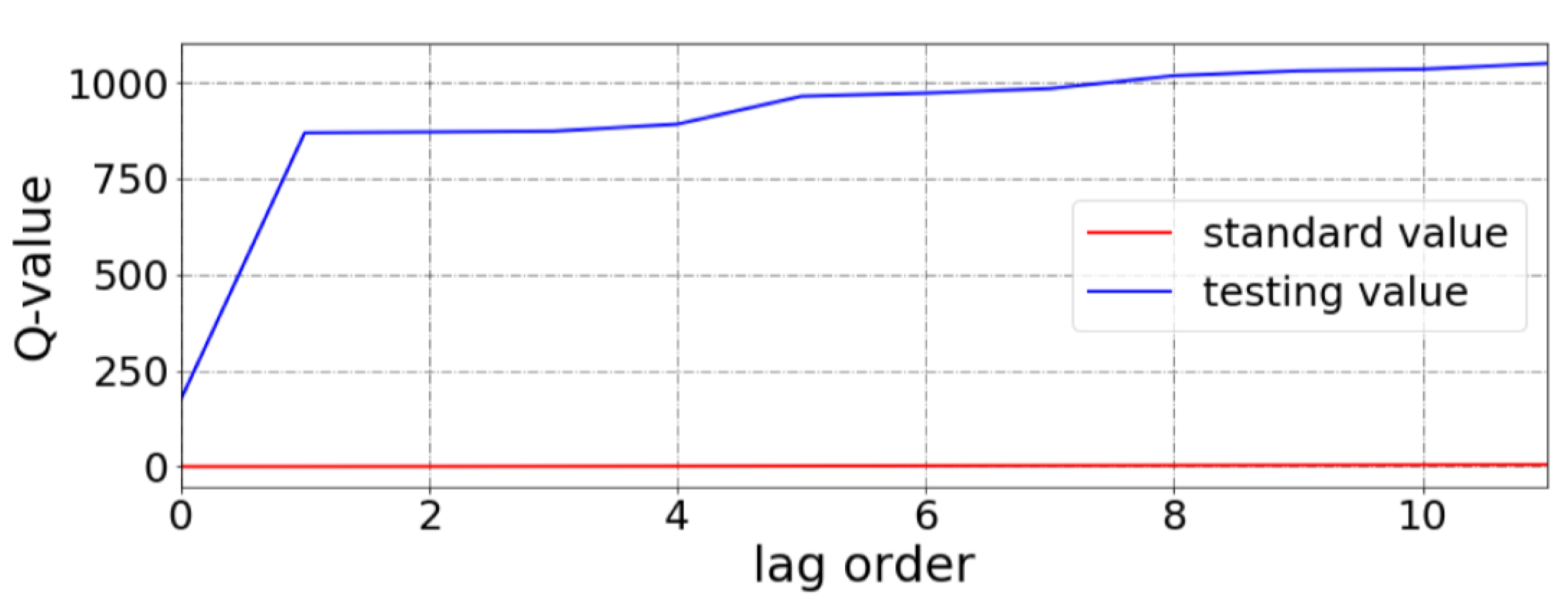
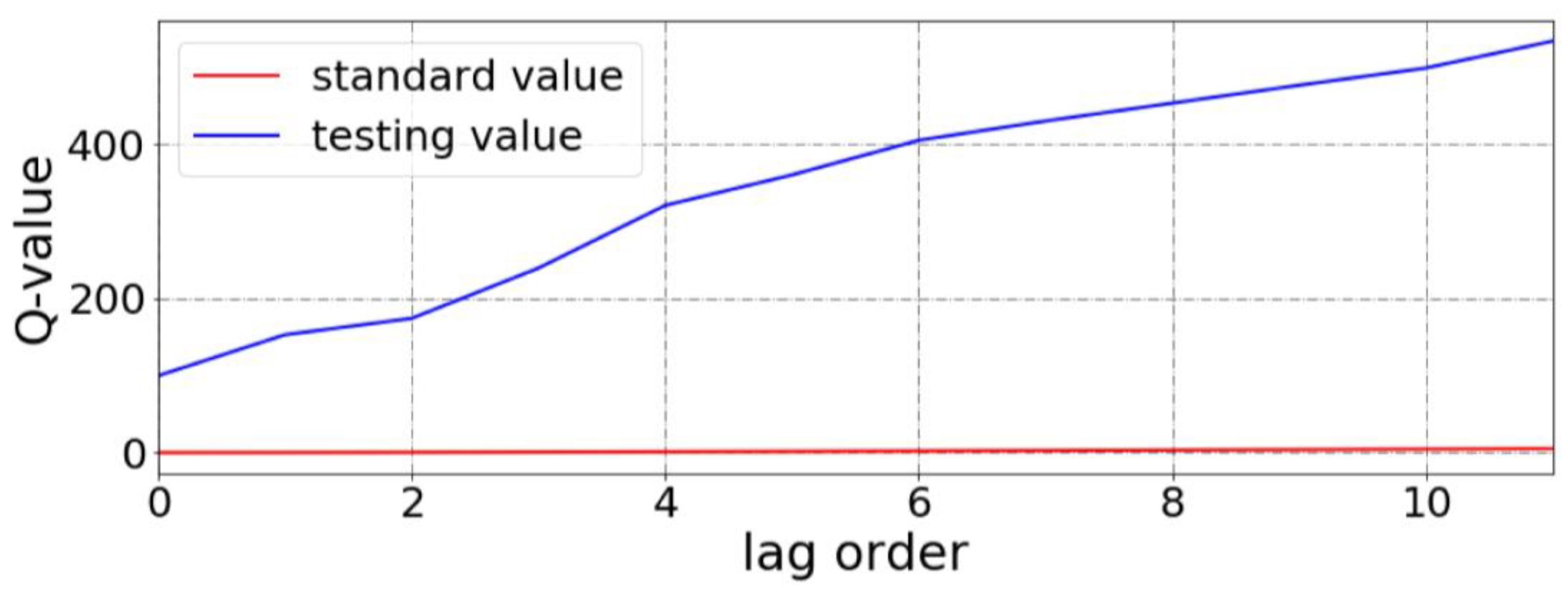
2.6. White Noise Test

The white noise series has no correlation between the values and is therefore meaningless to investigate. Stationary series usually have a short-term correlation which can be described by the autocorrelation coefficient. With the increase in the number of delay periods, the autocorrelation coefficient of the stationary series rapidly decays to 0.

In particular, the formula for calculating the correlation coefficient for delay is as follows:

$$\rho =\frac{{\displaystyle {\sum }_{i=1}^{n-t}(x_i-\upsilon )(x_{i+t}-\upsilon )}}{{\displaystyle {\sum }_{i=1}^n{(x_i-\upsilon )}^2}}$$

(34)

where $t$ is the delay period, $n$ is the number of the value and $\upsilon$ is the mean of all the values.

In a white noise series, the distribution of the autocorrelation coefficient will be:

$${\rho }_0~N(0,\frac{1}{n})$$

(35)

2.7. Extreme Gradient Boosting

The extreme gradient boosting (Xgboost) algorithm is applied to finish the integration task. The main steps are as follows.

Step 1: The objective function of the boosting method is defined.

For each regression tree, the model can be expressed as:

$$f_t(x)=w_{q_x}, w\in R^T. q:R^d\to 1,2\dots T$$

(36)

where $w$ represents the vector of the leaves and $q$ means the structure of the tree while $T$ is the number of leaf nodes in the tree. Then, the tree complexity can be expressed as:

$$\Omega (f_t)=\gamma T+\frac{1}{2}\lambda {\displaystyle {\sum }_{j=1}^T{w}_j^2}$$

(37)

where γ is the regular penalty of $L_1$, while λ is the regular penalty of $L_2$.

Step 2: A cycle is established.

Step 3: The gradient vector of the loss function of the $m-th$ iteration is calculated.

As with the traditional boosting tree model, the lifting model of Xgboost also uses residuals (or negative gradient direction). The difference is that the selection of split nodes is not necessarily the least square loss. Here, the goal function can be expressed as:

$$Ob{j}^{(t)}\cong {\displaystyle {\sum }_{i=1}^n\left[l(y_i,{\widehat{y}}_i^{(t-1)})+g_i{f}_t(x_i)+\frac{1}{2}{h}_i{f}_t^2(x_i)\right]}+\Omega (f_t)+C$$

(38)

Step 4: The Hessian matrix of the m-th iteration is calculated.

The objective function is only dependent on the first two derivatives of each data point on the error function. The reason for this is obvious. Since the previous objective function is only appropriate for the square loss function when seeking the optimal solution, it becomes very complicated for other loss functions. Through the transformation of the second-order Taylor expansion, the other solutions are solved in this way. Then, the objective function is transformed into the form of a leaf node in the $t-th$ tree:

$$Ob{j}^{(t)}\cong {\displaystyle {\sum }_{j=1}^T\left[({\displaystyle {\sum }_{i\in I_j}{g}_i})w_j+\frac{1}{2}({\displaystyle {\sum }_{i\in I_j}{h}_i+\lambda })w_j^2\right]}+\gamma T$$

(39)

where $I_j=i|q(x_i=j)$ means the sample $i$ lands on the $j-th$ leaf node and $w_j$ is the score of the $j-th$ leaf node. When the partial derivative of $w_j$ is found and its derivative function is made equal to 0, we have:

$$w_j^{\ast }=-\frac{G_j}{H_j+\lambda }$$

(40)

$$Obj=-\frac{1}{2}{\displaystyle {\sum }_{j=1}^T\frac{G_j^2}{H_j+\lambda }}+\gamma T$$

(41)

Step 5: The decision tree parameters for minimizing loss function are calculated.

Step 6: The weights of each base learner are combined to obtain the base learner model.

Additionally, this will be the loss function we need. Then, the estimate of the efficiency will be expressed in the form of the score:

$$Gain=\frac{1}{2}\left[\frac{G_L^2}{H_L+\lambda }+\frac{G_R^2}{H_R+\lambda }-\frac{{(G_L+G_R)}^2}{H_L+H_R}\right]-\gamma$$

(42)

In theory, the general gain will be the mixture of the score of the left and right sub-tree minus the score if the split is not applied.

Step 7: The basic learner models obtained from the loop are all added.

2.8. Gaussian Process

The Gaussian process is usually described by a function. If two points are: $x_0$ = 0, $x_1$ = 1, then their function values will satisfy a Gaussian distribution:

$$\left(\begin{array}{l}{y}_0\\ y_1\end{array}\right)~N\left(\left(\begin{array}{l}0\\ 0\end{array}\right),\left(\begin{array}{l}1\hspace{1em}0\\ 0\hspace{1em}1\end{array}\right)\right)$$

(43)

where $y_0$ and $y_1$ are the function values.

Then, we have the kernel function:

$$k(x,x^{\prime })=\exp (-{\Vert x-x^{\prime }\Vert }^2/2{\sigma }^2)$$

(44)

where $\sigma$ is the standard deviation.

This is seen as the distance. If there are N data points, these function values will satisfy the N-dimensional Gaussian distribution with the mean of 0. Each element in it corresponds to (K means covariance matrix):

$$K_{nm}=k(x_n,x_m)$$

(45)

Then, the Gaussian process can be applied to learn any function. Assuming a given $x$, $y$ follows:

$$p\left(y|x\right)=N(y|0,K)$$

(46)

where $K=k(x,x)$.

In the introduced training set, $x_{\#}$, $y_{\#}$ will be the joint conditional distribution ($y_{\ast }$ is the output):

$$\left(\begin{array}{l}{y}_{\#}\\ y_{\ast }\end{array}\right)~N\left(\left(\begin{array}{l}{0}_{\#}\\ 0_{\ast }\end{array}\right),\left(\begin{array}{l}{K}_{\#}\hspace{1em}{K}_{\ast }\\ K_{\ast }^T\hspace{1em}(K_{\ast },K_{\ast })\end{array}\right)\right)$$

(47)

Then, we have a conditional distribution ($x_{\ast }$ is the output):

$$p(y_{\ast }|x_{\ast },x,y)=N(y_{\ast }|{\mu }_{\ast },E_{\ast })$$

(48)

Here, ${\mu }_{\ast }$ and $E_{\ast }$ can be calculated through:

$${\mu }_{\ast }=K_{\ast }^T{K}^{-1}y$$

(49)

$$E_{\ast }=(K_{\ast },K_{\ast })-K_{\ast }^T{K}^{-1}{K}_{\ast }$$

(50)

3. Proposed Model and the Evaluation Criteria

This section gives the general procedure of the proposed model and the evaluation criteria used to assess the prediction ability.

3.1. Proposed Model

Figure 2 demonstrates the flowchart and the main parts are introduced as well:

(1)

CEEMDAN combined with AE is the first decomposition step where the raw data are decomposed in an effort to extract the features.

(2)

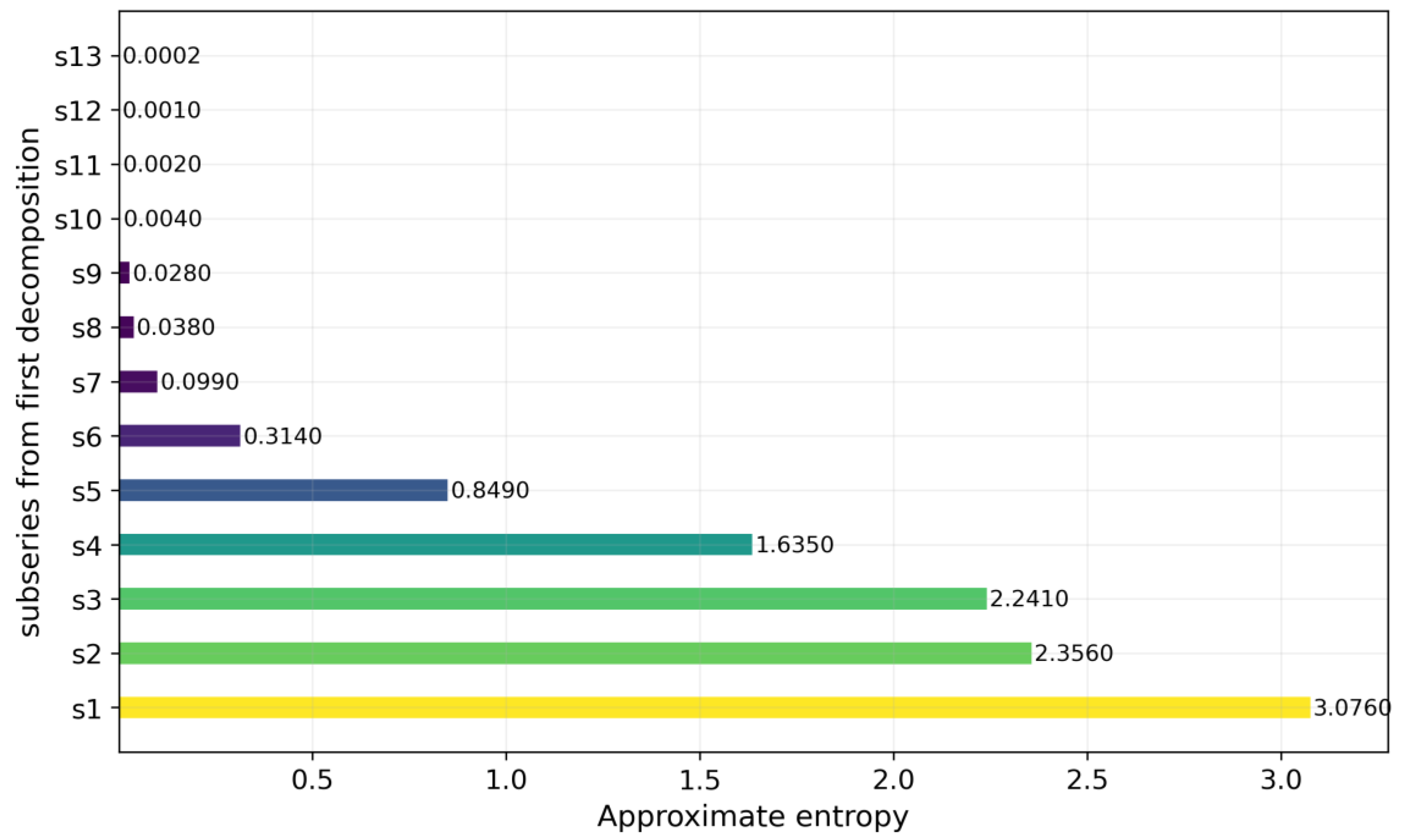
SSA decomposition is the secondary decomposition process where the focus is on the subsequence with the highest AE value. The first two steps are seen as the whole decomposition system which stresses the different features of the data series.

(3)

When the decomposition process is finished, the number of the subsequences will be too large which will bring a low efficiency in computation. Therefore, an auto encoder is used to realize the dimensionality reduction task to reduce the number of the subsequences.

(4)

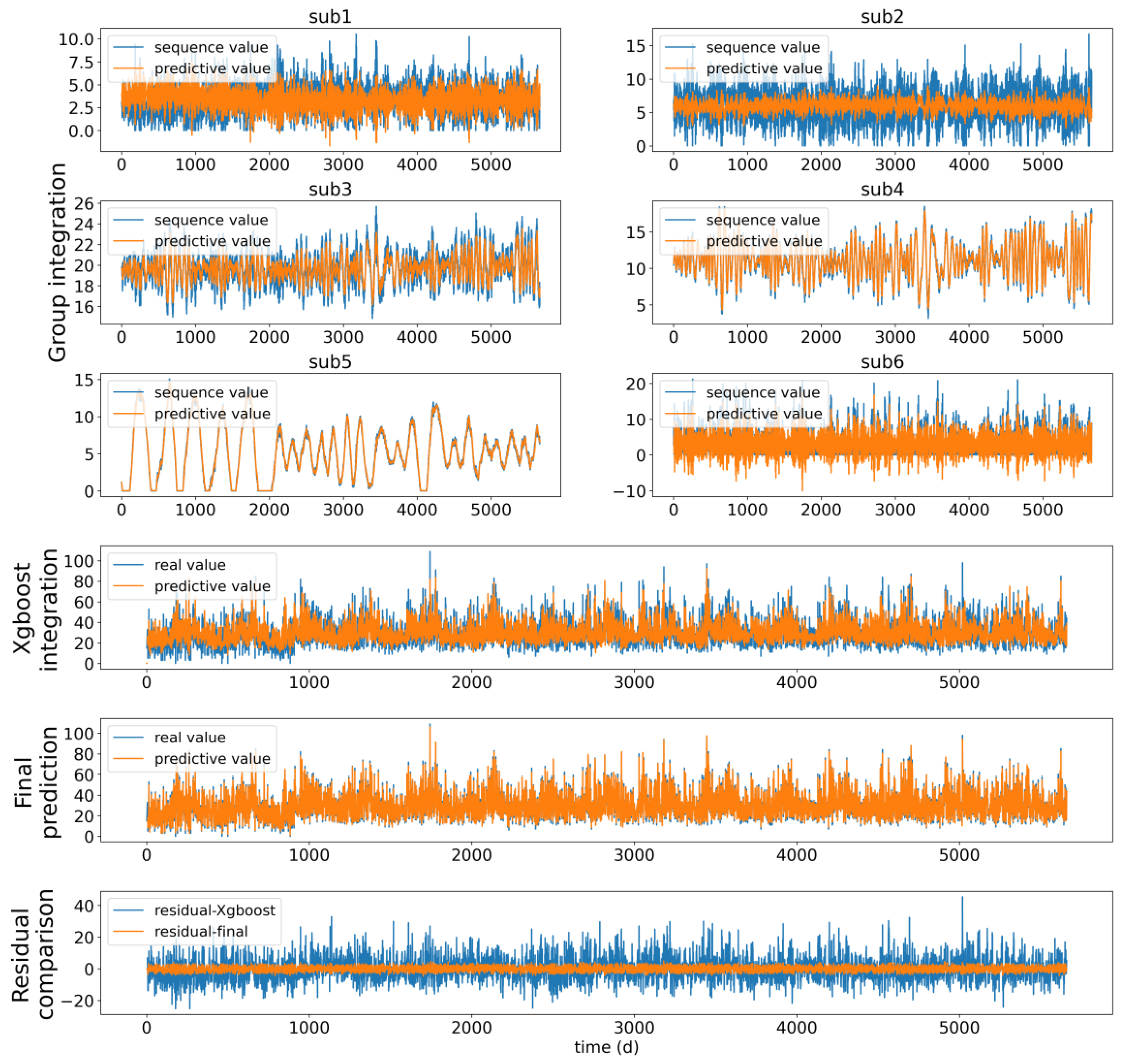
Each subsequence will go through the elastic neural network to generate the sub-result, after obtaining these sub-results, Xgboost will generate the first prediction result based on sub-results. This process can be seen as a two-step nonlinear learning process.

(5)

Error correction is another innovation in the proposed model, which can correct the first predictive results and achieve a higher accuracy. Here, the white noise test is used to verify whether the predictive results should be corrected.

(6)

The last step is to generate the interval prediction. GP has the ability of interval generation which will be used in this paper, and this will bring a high fault tolerance and low uncertainty.

3.2. Evaluation Criteria

There are five measures selected to assess the predicting ability of the models (see

Table 1. The formula of evaluation criteria.

Name	Equation
MAE	$\frac{1}{n_1}{\displaystyle \sum _{i=1}^{n_1^{}}\left|w(i)-\widehat{w}(i)\right|}$
RMSE	$\sqrt{\frac{1}{n_1}{\displaystyle \sum _{i=1}^{n_1}{(w(i)-\widehat{w}(i))}^2}}$
MAPE	$\frac{1}{n_1}{\displaystyle \sum _{i=1}^{n_1}\left|\frac{w(i)-\widehat{w}(i)}{w(i)}\right|\times 100\%}$
MWP	$\frac{1}{n_1}{\displaystyle \sum _{i=1}^{n_1}\frac{U(x_i)-L(x_i)}{r_i}}$
CP	$\frac{{\lambda }^{1-\mu }}{n_1}\times 100\%$

). Three of them are used for evaluating the point prediction performance, which are mean absolute error (MAE), root mean squared error (RMSE), and mean absolute percentage error (MAPE), respectively. Because the three indexes quantify the number of errors, the smaller is the better. The rest is coverage probability (CP) and mean width percentage (MWP), which are mainly used to evaluate the performance of interval prediction. The larger the CP is, the better the interval prediction is. The MWP value cannot be too large or small, otherwise there will not be a suitable interval.

In Table 1, $n_1$ is the sample number, $w(i)$ is the real wind speed at time point $i$ and $\widehat{w}(i)$ is the prediction speed, ${\lambda }^{1-\mu }$ is the number of the actual speed falling in the gap at the confidence of $1-\mu$; $U(x_i)$ and $L(x_i)$ are the upper/lower bounds; $r_i$ is the $i-th$ real value.

4. Case Study

4.1. Data Collection

This study applied data from four places which are Dingxin, Yongchang, Jingtai, and Wushan. They are, respectively, referred to case 1, case 2, case 3, and case 4. The four places are all located in Gansu, China. The data were sourced from the website of China Meteorological Data Service Center, http://data.cma.cn/ (accessed on 12 April 2022). The basic information of datasets is shown in

Table 2. The basic information of datasets.

Dataset	Dingxin	Wushan	Yongchang	Jingtai
Starting date	1 January 1955	1 January 1969	1 January 1960	1 October 1956
Ending date	31 December 2016	31 December 2016	31 December 2016	31 December 2016
Samples	22,645	17,531	20,819	21,975
Mean	30.790	29.740	29.157	25.677
Min	0	0	0	0
Max	143	103	139	127
Std.	16.398	12.358	13.970	15.082
Normal test	8136.28	2528.81	15,631.97	12,534.76

Std. means standard deviation; the normal test is Jarque-Bera test.

. It is apparently shown that the empirical distribution of the studied datasets is far away from normal distribution based on the results of a normal test. The standard deviation represents the fluctuation degree and it can be seen that the volatility in the four datasets was very close. The daily average wind speed was selected and 75% data were used as the training set and the rest was used as the test set (the ratio is 3:1).

4.2. Point Prediction

4.2.1. Case I: Wind Speed from Dingxin

The data series was firstly divided into subsequences using CEEMDAN. Then, for each subsequence, the AE value was calculated, as is shown in Figure 3.

It is obvious that s1 and s2 are apparently higher than others (which are larger than 2), so they were decomposed again, separately, through SSA. After the two-stage decomposition, the original data series was decomposed into 27 subseries. The subsequences were reconstructed through the auto encoder and the reconstructed sequences are shown in Figure 4.

Once the decomposition and dimension reconstruction were finished, the integration process was carried out. Firstly, an elastic neural network was employed in each subsequence to obtain the sub-result and then Xgboost was used to integrate all the sub-results into one prediction result. Subsequently, the white noise test was conducted on the residual series to determine whether to use an error correction strategy. The Q-values are shown in Figure 5 and clearly the residual series was proven not to be a white noise series.

For the residual correction part, Xgboost was applied again on the residual series. The process is described in Figure 6. To further demonstrate the necessity of residual correction, Figure 6 shows the comparison of the first residual series from Xgboost and the final residual series from error correction. It can be seen in the figure that the residual series after error correction was closer to zero than the previous one, which means the residual correction strategy can effectively improve accuracy.

The numerical results are shown in the next section.

Table 3. Parameters used in case 1.

	Sub 1	Sub 2	Sub 3	Sub 4	Sub 5	Sub 6
alpha	0.001	0.001	0.001	0.001	0.001	0.001
ratio	0.001	0.001	0.001	0.899	0.001	0.001
Xgboost-integration			Xgboost-residual correction
max_depth	subsample	colsample_bytree	max_depth	subsample	colsample_bytree
5	0.8	0.7	70	0.75	0.6

is the related parameters.

4.2.2. Case II: Test with Wind Speed from Wushan

The second dataset was from Wushan, China. The data series was firstly divided into subsequences using CEEMDAN. Then, for each subsequence, the AE value was calculated, as is shown in Figure 7.

The highest value was over 3, which was then decomposed again, separately, through SSA. When the process above was completed, the auto encoder was applied to carry out the dimension reconstruction, which is shown in Figure 8.

When the decomposition and dimension reconstruction were finished, the integration process was carried out. Similarly, the Q-values are shown in Figure 9 and they proved the necessity to carry out residual correction.

The integration process and the residual comparison are shown in Figure 10.

The measures were also calculated and listed as well.

Table 4. Parameters used in case 2.

	Sub 1	Sub 2	Sub 3	Sub 4	Sub 5
alpha	0.01	0.01	0.01	0.01	0.01
ratio	0.616	1	0.01	0.01	1
Xgboost-integration			Xgboost-residual correction
max_depth	subsample	colsample_bytree	max_depth	subsample	colsample_bytree
3	0.7	0.65	105	0.7	0.65

is the related parameters.

4.2.3. Case III: Test with Wind Speed from Yongchang

In case 3, the samples were from Yongchang, China. The original data series was firstly divided into subsequences using CEEMDAN. Then, for each subsequence, the AE value was calculated, as is shown in Figure 11.

The highest value was over 5, which was decomposed again, separately, through SSA. When the subsequences were prepared, the auto encoder was applied to carry out the dimension reconstruction work, which is shown in Figure 12.

When the decomposition and dimension reconstruction were finished, the integration process was carried out. The result of the test is shown in Figure 13.

After the residual correction part was completed, the final point prediction was generated and the process above is described in Figure 13. The detailed point prediction results are shown in Figure 14.

Table 5. Parameters used in case 3.

		Sub 1	Sub 2	Sub 3
alpha		0.01	0.01	0.01
ratio		0.192	0.01	1
Xgboost-integration			Xgboost-residual correction
max_depth	subsample	colsample_bytree	max_depth	subsample	colsample_bytree
12	0.75	0.85	100	0.5	0.8

is the related parameters.

4.2.4. Case IV: Test with Wind Speed from Jingtai

For the case of Jingtai, China, the original data series was firstly divided into subsequences using CEEMDAN. Then, for each subsequence, the AE value was calculated, as is shown in Figure 15.

The highest value was over 2.5, which was decomposed again, separately, through SSA. Then, the auto encoder was applied to reconstruct the dimension and the output subsequences’ number was 5, which is shown in Figure 16.

After integration, the white noise test showed the residual series was not noisy. The values are shown in Figure 17.

When the residual correction part was finished, the final point prediction result was generated. The process above is described in Figure 18.

The parameters are shown in

Table 6. Parameters used in case 4.

	Sub 1	Sub 2	Sub 3	Sub 4	Sub 5
alpha	0.01	0.01	0.01	0.01	0.04
ratio	0.01	1	0.01	0.01	0.01
Xgboost-integration			Xgboost-residual correction
max_depth	subsample	colsample_bytree	max_depth	subsample	colsample_bytree
13	0.55	0.7	110	0.6	0.5

.

4.3. Interval Prediction

GP was used as the interval forecast tool. Figure 19 displays the GP results of the four datasets as well as some related measures. The parameters are displayed in

Table 7. Parameters of cases used in GP.

	Mean	cov	lik
Case 1	1	−1,1,−7	5
Case 2	1	−5,6,−1	3
Case 3	1	−1,0,−7	5
Case 4	1	1,−3,−2	3

. The measures of the four cases are shown in

Table 8. Measures of models.

Model	Case	Measure
		RMSE	MAE	MAPE	CP	MWP
Proposed model	Case 1	0.02	0.01	5.74%	0.9993	1.3986
	Case 2	0.02	0.01	5.08%	0.9881	0.6960
	Case 3	0.02	0.01	5.96%	0.9992	0.3784
	Case 4	0.01	0.01	6.25%	0.9498	0.2422
CEEMDAN-elastic neural network -two-step Xgboost	Case 1	0.16	0.12	51.23%	0.7928	1.2404
	Case 2	0.12	0.09	37.11%	0.7850	0.7338
	Case 3	0.13	0.09	37.54%	1	5.0851
	Case 4	0.13	0.09	46.87%	1	3.6869
Elastic neural network- two-step Xgboost	Case 1	0.15	0.11	49.88%	0.6653	2.4638
	Case 2	0.12	0.09	35.93%	1	2.2888
	Case 3	0.12	0.08	34.47%	0.9590	4.4455
	Case 4	0.11	0.08	41.74%	1	2.8217
CEEMDAN-AE- SSA-AE-elastic neural network	Case 1	0.12	0.09	39.40%	0.9610	2.9545
	Case 2	0.08	0.07	29.03%	0.9400	1.6599
	Case 3	0.07	0.06	23.67%	0.9760	3.7672
	Case 4	0.08	0.09	29.03%	1	2.9151
CEEMDAN-AE- SSA-AE-elastic neural network- linear accumulation	Case 1	0.27	0.23	135.73%	1	9.0649
	Case 2	0.21	0.18	93.58%	0.9470	2.7619
	Case 3	0.25	0.23	78.50%	0.9560	4.5932
	Case 4	0.19	0.16	62.06%	0.9970	4.8145
CEEMDAN-AE- SSA-AE-elastic neural network- Xgboost integration	Case 1	0.08	0.06	24.28%	0.6797	0.0012
	Case 2	0.06	0.05	18.99%	0.7508	0.0013
	Case 3	0.04	0.03	12.56%	0.2810	0.0016
	Case 4	0.02	0.01	8.12%	0.1578	0.0019

.

4.4. Analysis and Discussion

In order to show the rationality of model construction, we designed the following comparative experiments: (1) The first model used a one-step decomposition which is different to our secondary decomposition model; (2) the second model discarded the whole decomposition process and directly built the model on the original dataset; (3) the third model contained the whole decomposition process, but the integration process only contained the elastic neural network; (4) the fourth model used linear accumulation to replace nonlinear integration; (5) the fifth model was designed to show the significance of residual correction and it was the proposed model without the residual correction process.

Based on the above comparative experiments, we can obtain the following conclusions:

(1)

The proposed model applies a secondary decomposition process which contains CEEMDAN and SSA while some existing studies only use one-step decomposition. For this reason, the first cases applied a one-step decomposition. The next steps remained the same as the proposed model. The RMSE and MAE values showed obvious increases with the secondary decomposition. More specifically, the RMSE values of the four cases were, respectively, 8 times, 6 times, 6.5 times and 13 times larger than that of the proposed model; the MAE values of the comparative model were also several times larger than the proposed one. The increase in the MAPE values was also apparent in the four cases and the value increased by 45.49%, 32.03%, 31.58%, and 40.62%, respectively. Then, for the interval prediction, the CP values of the first two cases decreased by about 0.2, while the MWP values increased by about 0.2 and 0.03. It can be seen that in the third and fourth cases, the CP values showed a slight increase while the MWP values showed a multifold increase. The experiment demonstrates that the one-step decomposition will neglect some information in the series which means the feature extraction still has room for improvement. Moreover, it proves that the two-step decomposition is necessary.

(2)

There are a large number of studies investigating the study process on the original dataset, so in the second model, the whole decomposition process was deleted entirely as a comparative group. The RMSE values of the second comparative model were dozens of times larger than the proposed model as well as the MAE values in all cases. Similarly, the MAPE values were several times larger than the proposed model’s. In addition, the CP value of the first case showed an apparent decrease by 0.334, and the MWP value increased to 2.4638. For the next three cases, the CP values showed no great difference, but the MWP values all became far from satisfactory. Obviously, using the original dataset directly means that all the features are given the same weight, which can greatly affect the prediction ability in practice.

(3)

The third model turned the original two-step learning process to a one-step integration. For certain, the process became easier to operate, but the accuracy and fault tolerance were both influenced. The most obvious changes were the increase in the MAPE value in case 1 by 33.66% and the increase in the MWP value in case 3, which was multiplied 9.96 times. The simplified process brought not only the decline in the point prediction accuracy, but also a negative effect on the certainty. Sometimes, a simple one-step integration does offer a good performance, but it also causes risks that the features are not fully captured and the learning process is insufficient. Thus, in an effort to complete the learning process and pay as much attention as possible to all the features, it is highly recommended to apply a two-step learning process.

(4)

The proposed model applies nonlinear integration as an important process in the point prediction period. In some classic methods, linear accumulation is always utilized, so the fourth model replaced the Xgboost integration with linear accumulation. It was learned from the results that the accuracy greatly decreased. The RMSE values were much larger than that in the proposed model in the four cases. The MAE values increased by the similar multiples accordingly. The MAPE values showed a distinct increase as well and the values of the four cases increased by 129.99%, 88.50%, 72.54% and 55.81%, respectively. Meanwhile, in the interval prediction process, differences in the CP values were not really evident, but when it came to MWP values, the values increased by 7.6663, 2.0659, 4.2418 and 4.5723, which means the gap between the boundaries widened and this will bring large uncertainty. Linear integration takes the least time to operate and it is the easiest way to generate results, but doing this means the ignorance of nonlinear features, and, as a result, the prediction accuracy is far from satisfactory.

(5)

Finally, as the residual correction strategy is another notable part in the proposed model, to further demonstrate the significance of this, the fifth model eliminated the residual correction process. Drawn from the table, the RMSE values of the four cases increased by 0.06, 0.04, 0.02, and 0.01, respectively, together with an increase in the MAE values in the first three cases, by 0.05, 0.04, and 0.02, respectively. While for the interval prediction, the CP values showed a great decline, and the gap narrowed further, with decreases of 1165.50 times, 535.38 times, 236.50 times, and 127.47 times in four cases. It has been said that MWP values cannot be too large or too small, and in this experiment, the MWP with too small values will turn the interval prediction to the results that are quite alike with the point prediction. In other words, the residual correction must not be neglected. The residual series is always neglected by researchers while, as a matter of fact, some features in the residual series remain unnoticed. The application of the residual correction strategy means the capturing of all the possible information and, by doing this, the performance will be the most precise.

To sum up, the proposed model shows improvement in many aspects which are often not given much attention. In this model, the data is decomposed fully to separate the features and a two-step learning process captures the nonlinear features to a large extent. In addition, the residual series is given the correct attention. According to the results of the experiments above, these techniques are noteworthy and effective.

5. Conclusions

The accurate prediction of wind speed is of great significance. This study proposed a two-stage decomposition multi-scale nonlinear ensemble model and this model contains a secondary decomposition feature reconstruction process and a two-stage nonlinear process including a residual correction strategy. The proposed model is capable of providing point and interval prediction results. Both the case studies and the comparison models show that the proposed model can improve not only the accuracy of the point prediction but the performance of interval prediction.

The proposed model combines various methods effectively and reasonably and it can be applied in other fields of data prediction and trend modification. In addition, the proposed model also has room for improvement. For example, some different integration and decomposition methods can be applied as well.

References

1. Chinmoy, L.; Iniyan, S.; Goic, R. Modeling wind power investments, policies and social benefits for deregulated electricity market—A review. Appl. Energy 2019, 242, 364–377. [Google Scholar] [CrossRef]
2. Zhang, Y.G.; Chen, B.; Pan, G.F.; Zhao, Y. A novel hybrid model based on VMD-WT and PCA-BP-RBF neural network for short-term wind speed forecasting. Energy Convers. Manag. 2019, 195, 180–197. [Google Scholar] [CrossRef]
3. Chen, C.; Liu, H. Dynamic ensemble wind speed prediction model based on hybrid deep reinforcement learning. Adv. Eng. Inform. 2021, 48, 101290. [Google Scholar] [CrossRef]
4. Liu, H.; Yu, C.M.; Yu, C.Q.; Chen, C.; Wu, H.P. A novel axle temperature forecasting method based on decomposition, reinforcement learning optimization and neural network. Adv. Eng. Inform. 2020, 44, 101089. [Google Scholar] [CrossRef]
5. Huang, N.E.; Shen, Z.; Long, S.R.; Wu, M.C.; Shih, H.H.; Zheng, Q. The empirical mode decomposition and the Hilbert spectrum for nonlinear and non-stationary time series analysis. Proc. R. Soc. Lond. Ser. A Math. Phys. Eng. Sci. 1998, 454, 903–995. [Google Scholar] [CrossRef]
6. Ren, Y.; Suganthan, P.N.; Srikanth, N. A Comparative Study of Empirical Mode Decomposition-Based Short-Term Wind Speed Forecasting Methods. IEEE Trans. Sustain. Energy 2017, 6, 236–244. [Google Scholar] [CrossRef]
7. Zhou, J.G.; Xu, X.L.; Huo, X.J.; Li, Y.S. Forecasting Models for Wind Power Using Extreme-Point Symmetric Mode Decomposition and Artificial Neural Networks. Sustainability 2019, 11, 650. [Google Scholar] [CrossRef] [Green Version]
8. Fei, S.W. A hybrid model of EMD and multiple-kernel RVR algorithm for wind speed prediction. Int. J. Electr. Power Energy Syst. 2016, 78, 910–915. [Google Scholar] [CrossRef]
9. Ye, R.; Suganthan, P.N.; Srikanth, N. A Novel Empirical Mode Decomposition With Support Vector Regression for Wind Speed Forecasting. IEEE Trans. Neural Netw. Learn. Syst. 2016, 27, 1793–1798. [Google Scholar] [CrossRef]
10. Qolipour, M.; Mostafaeipour, A.; Mohammad, S.M.; Arabnia, H.R. Prediction of wind speed using a new Grey-extreme learning machine hybrid algorithm: A case study. Energy Environ. 2019, 30, 44–62. [Google Scholar] [CrossRef]
11. Cheng, Z.S.; Wang, J.Y. A new combined model based on multi-objective salp swarm optimization for wind speed forecasting. Appl. Soft Comput. 2020, 92, 106294. [Google Scholar] [CrossRef]
12. Huang, Y.S.; Liu, S.J.; Yang, L. Wind Speed Forecasting Method Using EEMD and the Combination Forecasting Method Based on GPR and LSTM. Sustainability 2018, 10, 3693. [Google Scholar] [CrossRef] [Green Version]
13. Yang, Z.S.; Wang, J. A combination forecasting approach applied in multistep wind speed forecasting based on a data processing strategy and an optimized artificial intelligence algorithm. Appl. Energy 2018, 230, 1108–1125. [Google Scholar] [CrossRef]
14. Liu, H.; Mi, X.W.; Li, Y.F. Comparison of two new intelligent wind speed forecasting approaches based on Wavelet Packet Decomposition, Complete Ensemble Empirical Mode Decomposition with Adaptive Noise and Artificial Neural Networks. Energy Convers. Manag. 2018, 155, 188–200. [Google Scholar] [CrossRef]
15. Dragomiretskiy, K.; Zosso, D. Variational Mode Decomposition. IEEE Trans Signal Process. 2014, 62, 531–544. [Google Scholar] [CrossRef]
16. Fu, W.L.; Wang, K.; Zhou, J.Z.; Xu, Y.H.; Tan, J.W.; Chen, T. A Hybrid Approach for Multi-Step Wind Speed Forecasting Based on Multi-Scale Dominant Ingredient Chaotic Analysis, KELM and Synchronous Optimization Strategy. Sustainability 2019, 11, 1804. [Google Scholar] [CrossRef] [Green Version]
17. Wu, Q.L.; Lin, H.X. Short-Term Wind Speed Forecasting Based on Hybrid Variational Mode Decomposition and Least Squares Support Vector Machine Optimized by Bat Algorithm Model. Sustainability 2019, 11, 652. [Google Scholar] [CrossRef] [Green Version]
18. Moreno, S.R.; Mariani, V.C.; Coelho, L.D. Hybrid multi-stage decomposition with parametric model applied to wind speed forecasting in Brazilian Northeast. Renew. Energy 2021, 164, 1508–1526. [Google Scholar] [CrossRef]
19. Shukur, B.O.; Lee, M.H. Daily wind speed forecasting through hybrid KF-ANN model based on ARIMA. Renew. Energy 2015, 76, 637–647. [Google Scholar] [CrossRef]
20. Aasim, S.S.; Mohapatra, A. Repeated wavelet transform based ARIMA model for very short-term wind speed forecasting. Renew. Energy 2019, 136, 758–768. [Google Scholar] [CrossRef]
21. Sharma, S.K.; Ghosh, S. Short-term wind speed forecasting: Application of linear and non-linear time series models. Int. J. Green Energy 2016, 13, 1490–1500. [Google Scholar] [CrossRef]
22. Li, L.X.; Miao, S.H.; Tu, Q.Y.; Duan, S.M.; Li, Y.W.; Han, J. Dynamic dependence modelling of wind power uncertainty considering heteroscedastic effect. Int. J. Electr. Power Energy Syst. 2020, 116, 105556. [Google Scholar] [CrossRef]
23. Lucheroni, C.; Boland, J.; Ragno, C. Scenario generation and probabilistic forecasting analysis of spatio-temporal wind speed series with multivariate autoregressive volatility models. Appl. Energy 2019, 239, 1226–1241. [Google Scholar] [CrossRef]
24. Baomar, H.; Bentley, P.J. Autonomous flight cycles and extreme landings of airliners beyond the current limits and capabilities using artificial neural networks. Appl. Intell. 2021, 51, 6349–6375. [Google Scholar] [CrossRef]
25. Luo, X.J.; Oyedele, L.O.; Ajayi, A.O.; Monyei, C.G.; Akinade, O.O.; Akanbi, L.A. Development of an IoT-based big data platform for day-ahead prediction of building heating and cooling demands. Adv. Eng. Inform. 2019, 41, 100926. [Google Scholar] [CrossRef]
26. Zhang, Y.G.; Pan, G.F.; Zhang, C.H.; Zhao, Y. Wind speed prediction research with EMD-BP based on Lorenz disturbance. J. Electr. Eng. 2019, 70, 198–207. [Google Scholar] [CrossRef] [Green Version]
27. Ren, C.; An, N.; Wang, J.Z.; Li, L.; Hu, B.; Shang, D. Optimal parameters selection for BP neural network based on particle swarm optimization: A case study of wind speed forecasting. Knowl.-Based Syst. 2014, 56, 226–239. [Google Scholar] [CrossRef]
28. Liu, H.; Tian, H.Q.; Li, Y.F.; Zhang, L. Comparison of four Adaboost algorithm based artificial neural networks in wind speed predictions. Energy Convers. Manag. 2015, 92, 67–81. [Google Scholar] [CrossRef]
29. Wang, S.X.; Zhang, N.; Wu, L.; Wang, Y.M. Wind speed forecasting based on the hybrid ensemble empirical mode decomposition and GA-BP neural network method. Renew. Energy 2016, 94, 629–636. [Google Scholar] [CrossRef]
30. Jiang, P.; Li, R.R.; Zhang, K.Q. Two combined forecasting models based on singular spectrum analysis and intelligent optimized algorithm for short-term windspeed. Neural Comput. Appl. 2016, 30, 1–19. [Google Scholar] [CrossRef]
31. Zhang, C.; Wei, H.K.; Xie, L.P.; Shen, Y.; Zhang, K.J. Direct interval forecasting of wind speed using radial basis function neural networks in a multi-objective optimization framework. Neurocomputing 2016, 205, 53–63. [Google Scholar] [CrossRef]
32. Dalibor, P.; Shahaboddin, S.; Nor, B.A.; Hadi, S.; Ainuddin, W.A.W.; Milan, P.; Erfan, Z.; Seyed, M.A.M. An appraisal of wind speed distribution prediction by soft computing methodologies: A comparative study. Energy Convers. Manag. 2014, 84, 133–139. [Google Scholar] [CrossRef]
33. Zhang, Y.G.; Zhang, C.H.; Sun, J.B.; Guo, J.J. Improved Wind Speed Prediction Using Empirical Mode Decomposition. Adv. Electr. Comput. Eng. 2018, 18, 3–10. [Google Scholar] [CrossRef]
34. Wu, Z.Q.; Jia, W.J.; Zhao, L.R.; Wu, C.H. Maximum wind power tracking based on cloud RBF neural network. Renew. Energy 2016, 86, 466–472. [Google Scholar] [CrossRef]
35. Song, J.J.; Wang, J.Z.; Lu, H.Y. A novel combined model based on advanced optimization algorithm for short-term wind speed forecasting. Appl. Energy 2018, 215, 643–658. [Google Scholar] [CrossRef]
36. Thoranin, S. A new class of MODWT-SVM-DE hybrid model emphasizing on simplification structure in data pre-processing: A case study of annual electricity consumptions. Appl. Soft Comput. 2017, 54, 150–163. [Google Scholar] [CrossRef]
37. Fu, C.; Li, G.Q.; Lin, K.P.; Zhang, H.J. Short-Term Wind Power Prediction Based on Improved Chicken Algorithm Optimization Support Vector Machine. Sustainability 2019, 11, 512. [Google Scholar] [CrossRef] [Green Version]
38. Zhao, H.R.; Zhao, H.R.; Guo, S. Short-Term Wind Electric Power Forecasting Using a Novel Multi-Stage Intelligent Algorithm. Sustainability 2018, 10, 881. [Google Scholar] [CrossRef] [Green Version]
39. Yang, J.X. A novel short-term multi-input-multi-output prediction model of wind speed and wind power with LSSVM based on improved ant colony algorithm optimization. Cluster Comput. 2019, 22, S3293–S3300. [Google Scholar] [CrossRef]
40. Sun, W.; Liu, M.H.; Liang, Y. Wind Speed Forecasting Based on FEEMD and LSSVM Optimized by the Bat Algorithm. Energies 2015, 8, 6585–6607. [Google Scholar] [CrossRef] [Green Version]
41. Zhang, X.; Yan, M.; Xie, B.L.; Yang, H.Q.; Ma, H. An automatic real-time bus schedule redesign method based on bus arrival time prediction. Adv. Eng. Inform. 2021, 48, 101295. [Google Scholar] [CrossRef]
42. Zheng, H.; Wu, Y.H. A XGBoost Model with Weather Similarity Analysis and Feature Engineering for Short-Term Wind Power Forecasting. Appl. Sci. 2019, 9, 3019. [Google Scholar] [CrossRef] [Green Version]
43. Cai, R.; Xie, S.; Wang, B.Z.; Yang, R.J.; Xu, D.S.; He, Y. Wind Speed Forecasting Based on Extreme Gradient Boosting. IEEE Access. 2020, 8, 175063–175069. [Google Scholar] [CrossRef]
44. Chakraborty, D.; Elhegazy, H.; Elzarka, H.; Gutierrez, L. A novel construction cost prediction model using hybrid natural and light gradient boosting. Adv. Eng. Inform. 2020, 46, 101201. [Google Scholar] [CrossRef]
Figure 1. Auto encoder process.
Atmosphere 14 00395 g001
Figure 2. Flowchart of the proposed model.
Atmosphere 14 00395 g002
Figure 3. AE calculation.
Atmosphere 14 00395 g003
Figure 4. The six subfigures represent six subsequences which are generated through decomposition and dimension reduction from the original time series in case 1.
Atmosphere 14 00395 g004
Figure 5. Box_Ljung value of each lag order.
Atmosphere 14 00395 g005
Figure 6. The first six subfigures are the point prediction results of subseries. The seventh subfigure titled “Xgboost integration” shows the integrated results. The eighth subfigure represents the final point prediction results which are generated based on the Xgboost integration and error correction strategy. The last subfigure is the residual comparison between the model with error correction strategy and the model without it. All the experimental results here used data in case 1.
Atmosphere 14 00395 g006
Figure 7. AE calculation.
Atmosphere 14 00395 g007
Figure 8. The five subfigures represent five subsequences which are generated through decomposition and dimension reduction from the original time series in case 2.
Atmosphere 14 00395 g008
Figure 9. Box_Ljung value of each lag order.
Atmosphere 14 00395 g009
Figure 10. The first five subfigures are the point prediction results of subseries. The sixth subfigure titled “Xgboost integration” shows the integrated results. The seventh subfigure represents the final point prediction results which are generated based on the Xgboost integration and error correction strategy. The last subfigure is the residual comparison between the model with error correction strategy and the model without it. All the experimental results here used data in case 2.
Atmosphere 14 00395 g010
Figure 11. CEEMDAN and AE calculation.
Atmosphere 14 00395 g011
Figure 12. The three subfigures represent three subsequences which are generated through decomposition and dimension reduction from the original time series in case 3.
Atmosphere 14 00395 g012
Figure 13. Box_Ljung value of each lag order.
Atmosphere 14 00395 g013
Figure 14. The first three subfigures are the point prediction results of subseries. The fourth subfigure titled “Xgboost integration” shows the integrated results. The fifth subfigure represents the final point prediction results which are generated based on the Xgboost integration and error correction strategy. The last subfigure is the residual comparison between the model with error correction strategy and the model without it. All the experimental results here used data in case 3.
Atmosphere 14 00395 g014
Figure 15. CEEMDAN and AE calculation.
Atmosphere 14 00395 g015
Figure 16. The five subfigures represent five subsequences which are generated through decomposition and dimension reduction from the original time series in case 4.
Atmosphere 14 00395 g016
Figure 17. Box_Ljung value of each lag order.
Atmosphere 14 00395 g017
Figure 18. The first five subfigures are the point prediction results of subseries. The sixth subfigure titled “Xgboost integration” shows the integrated results. The seventh subfigure represents the final point prediction results which are generated based on the Xgboost integration and error correction strategy. The last subfigure is the residual comparison between the model with error correction strategy and the model without it. All the experimental results here used data in case 4.
Atmosphere 14 00395 g018
Figure 19. The interval prediction estimate of four cases.
Atmosphere 14 00395 g019