
A Comparative Study of Deep Learning Models on Tropospheric Ozone Forecasting Using Feature Engineering Approach

Abstract
:1. Introduction
2. Material and Methods
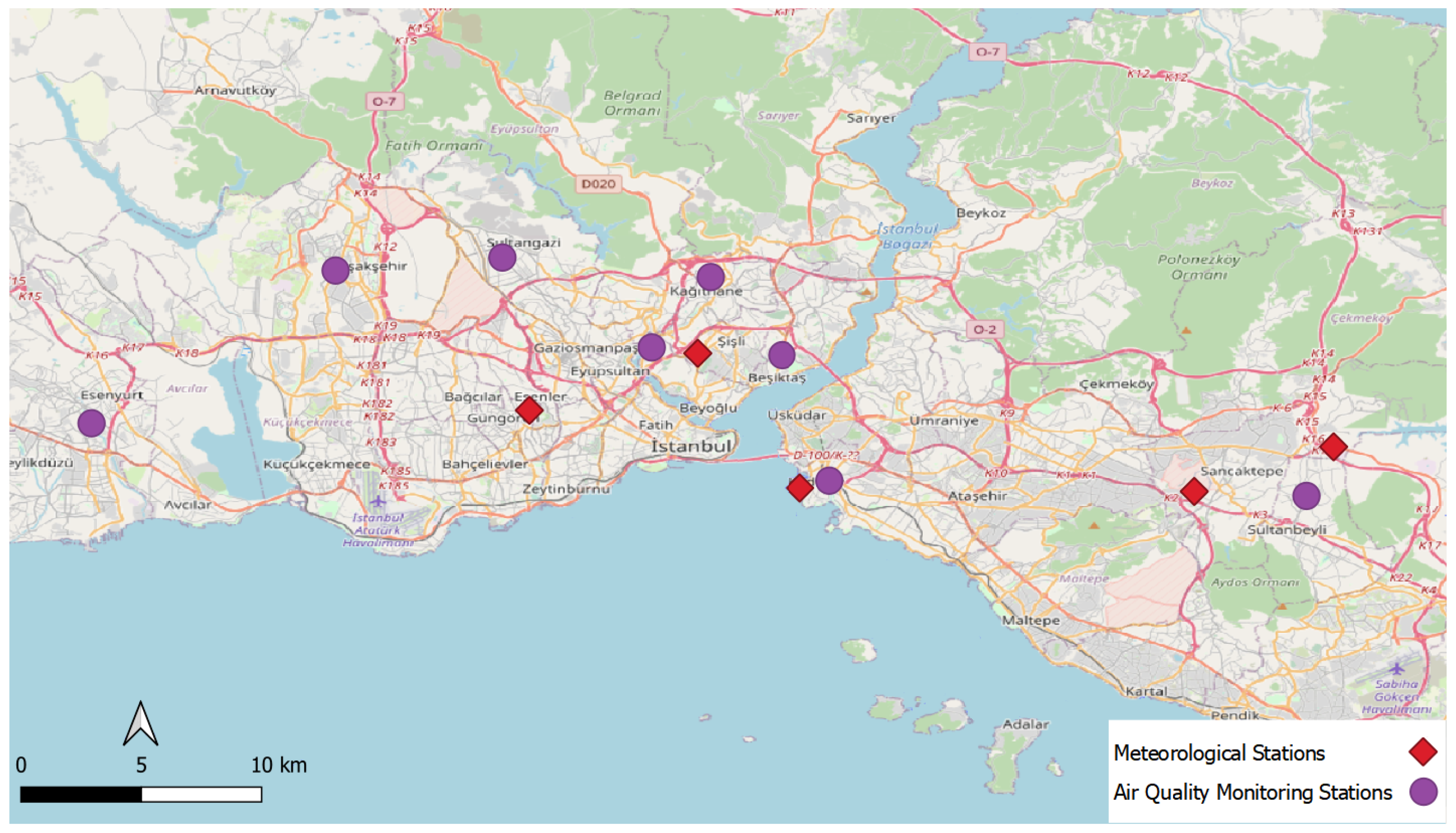
2.1. Study Area
2.2. Data Preprocessing
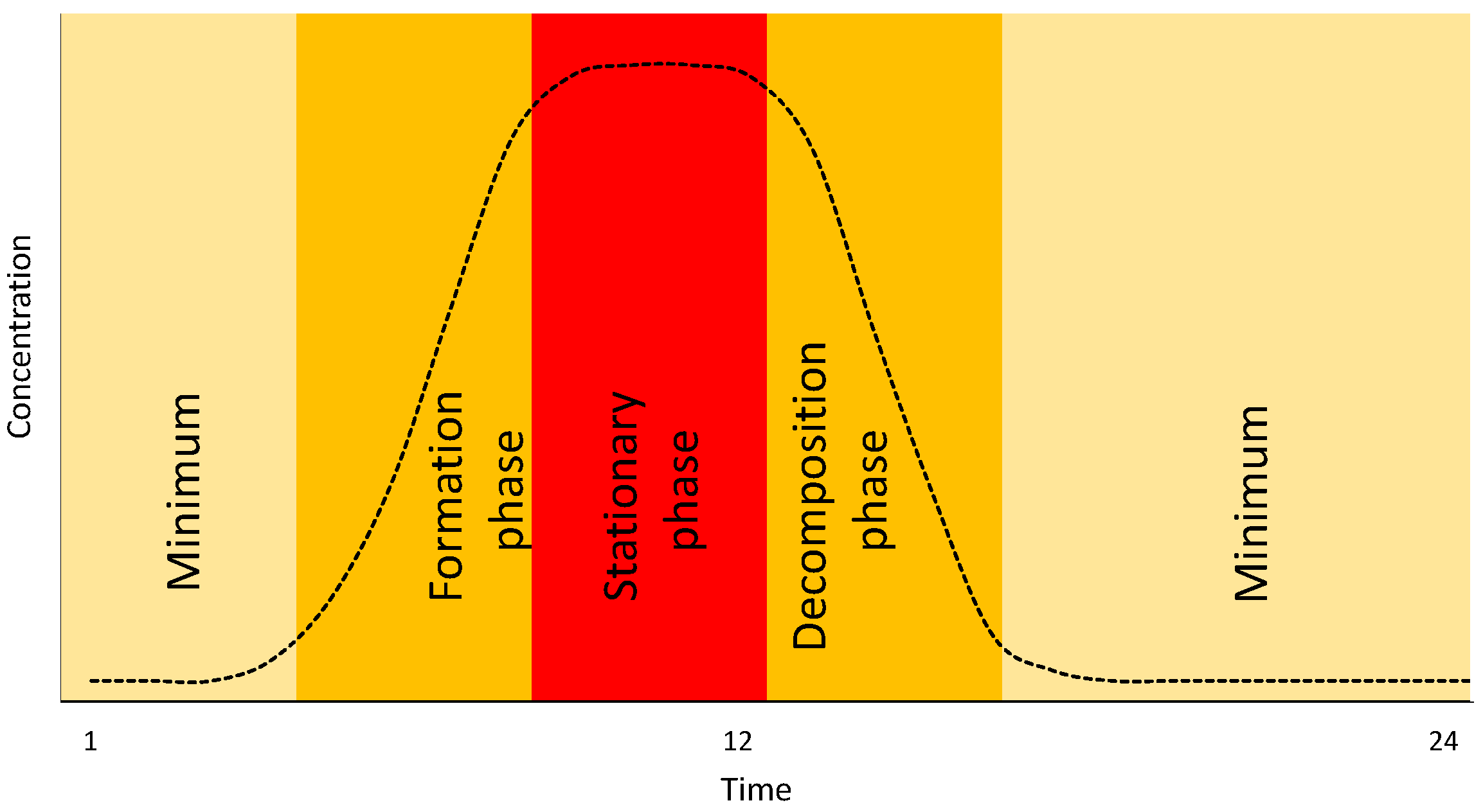
2.3. Dataset Analysis and Feature Engineering
2.4. Proposed Neural Networks Models
2.4.1. MLP Model
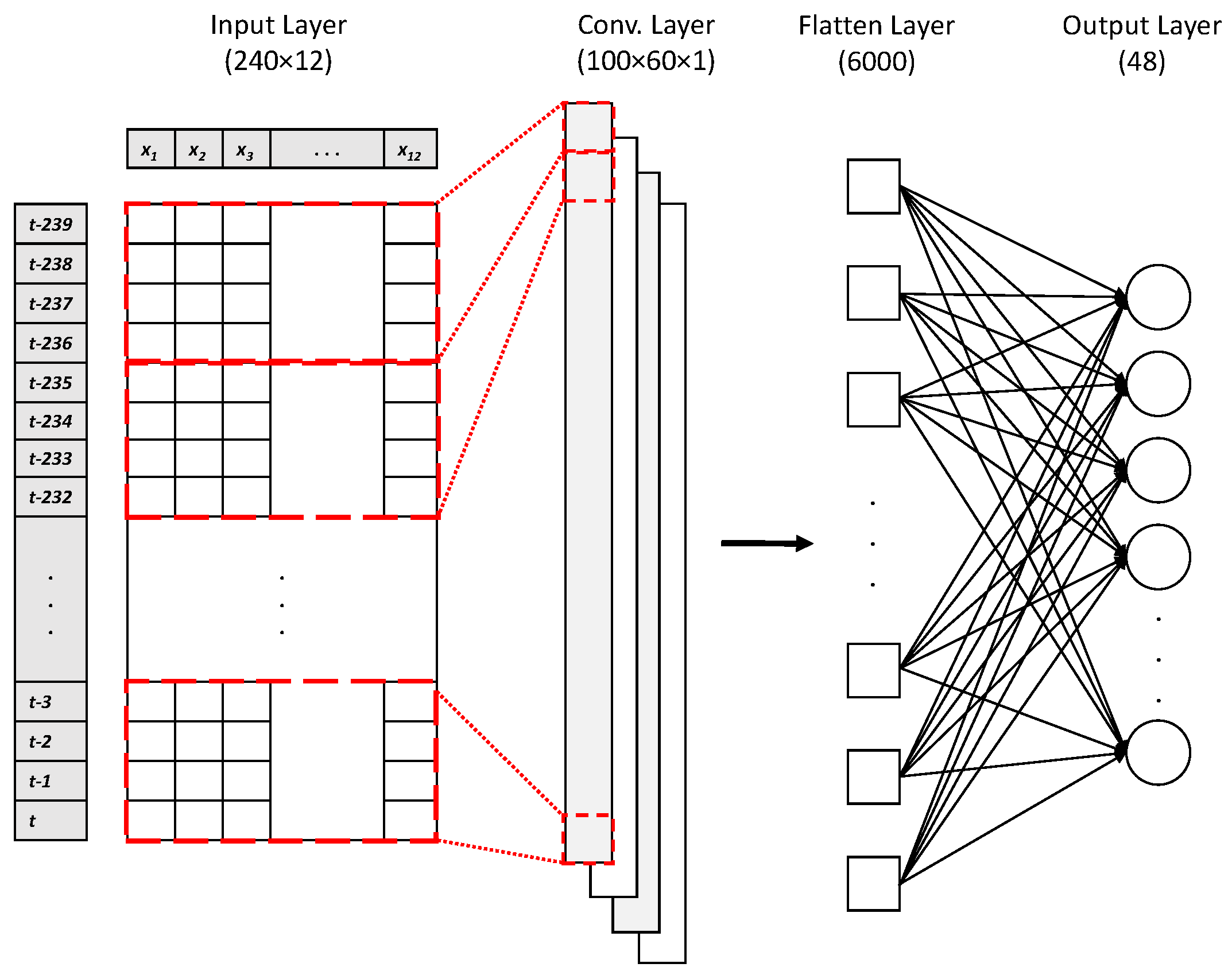
2.4.2. CNN Model
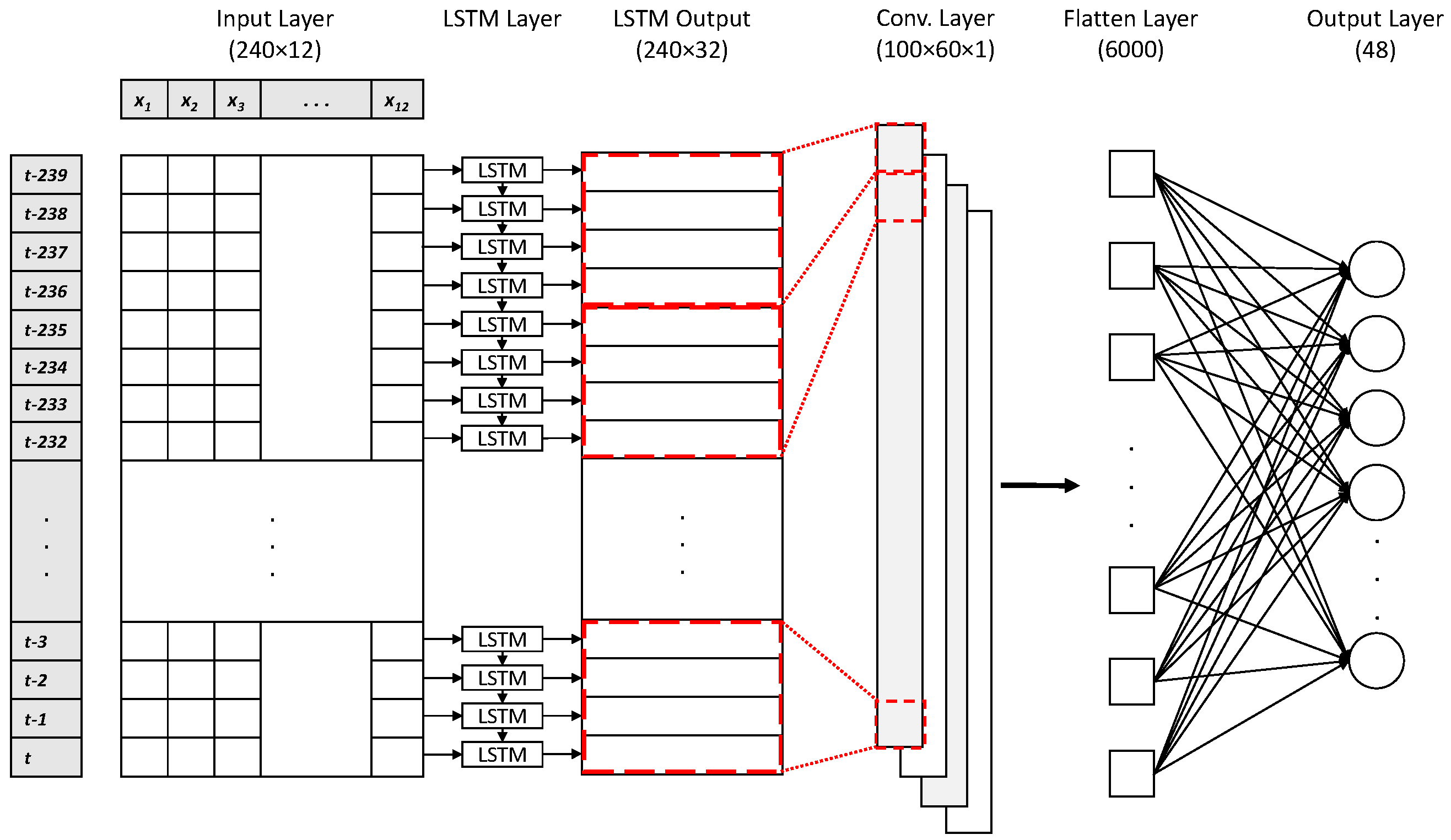
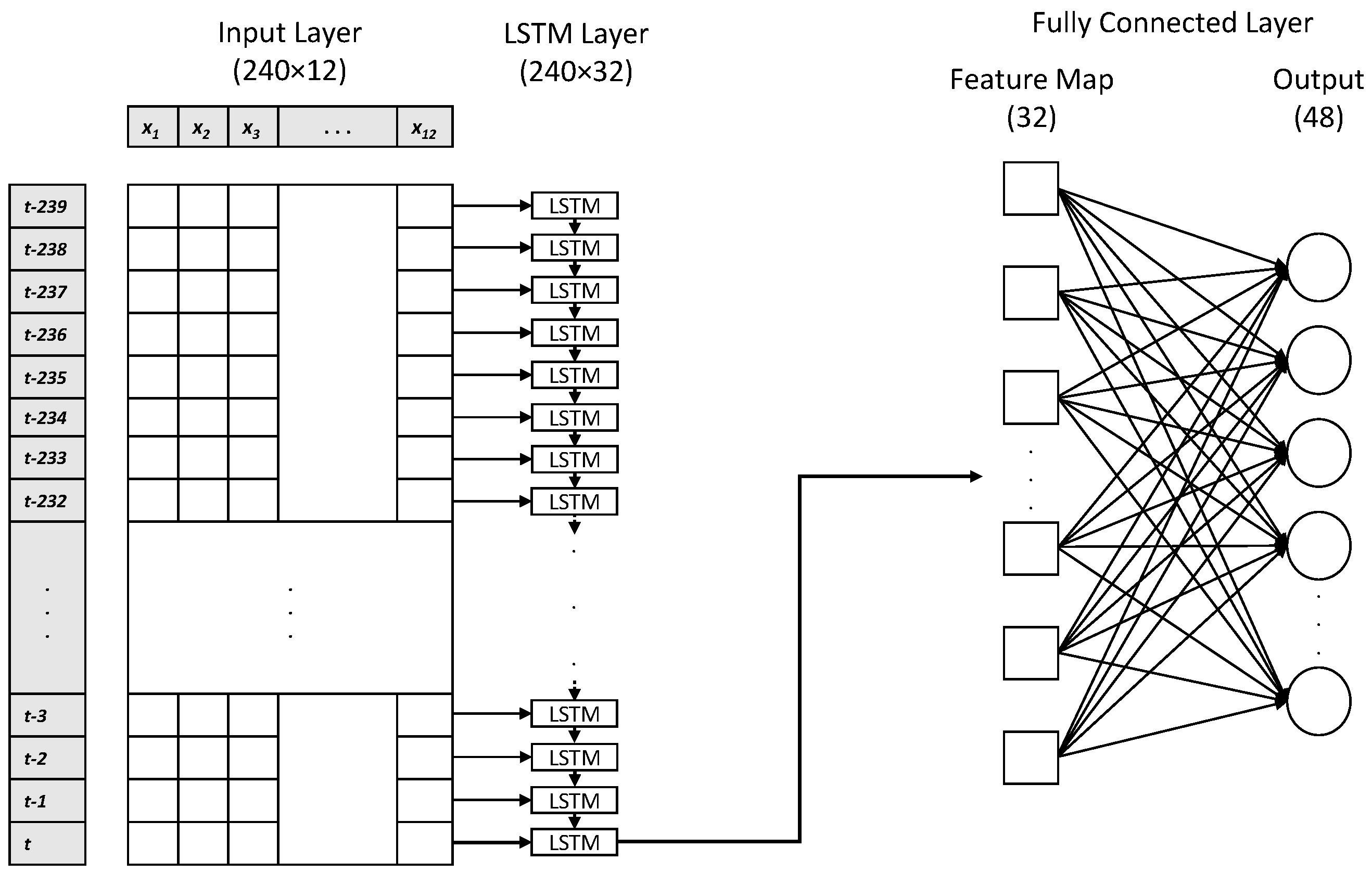
2.4.3. LSTM-CNN Model
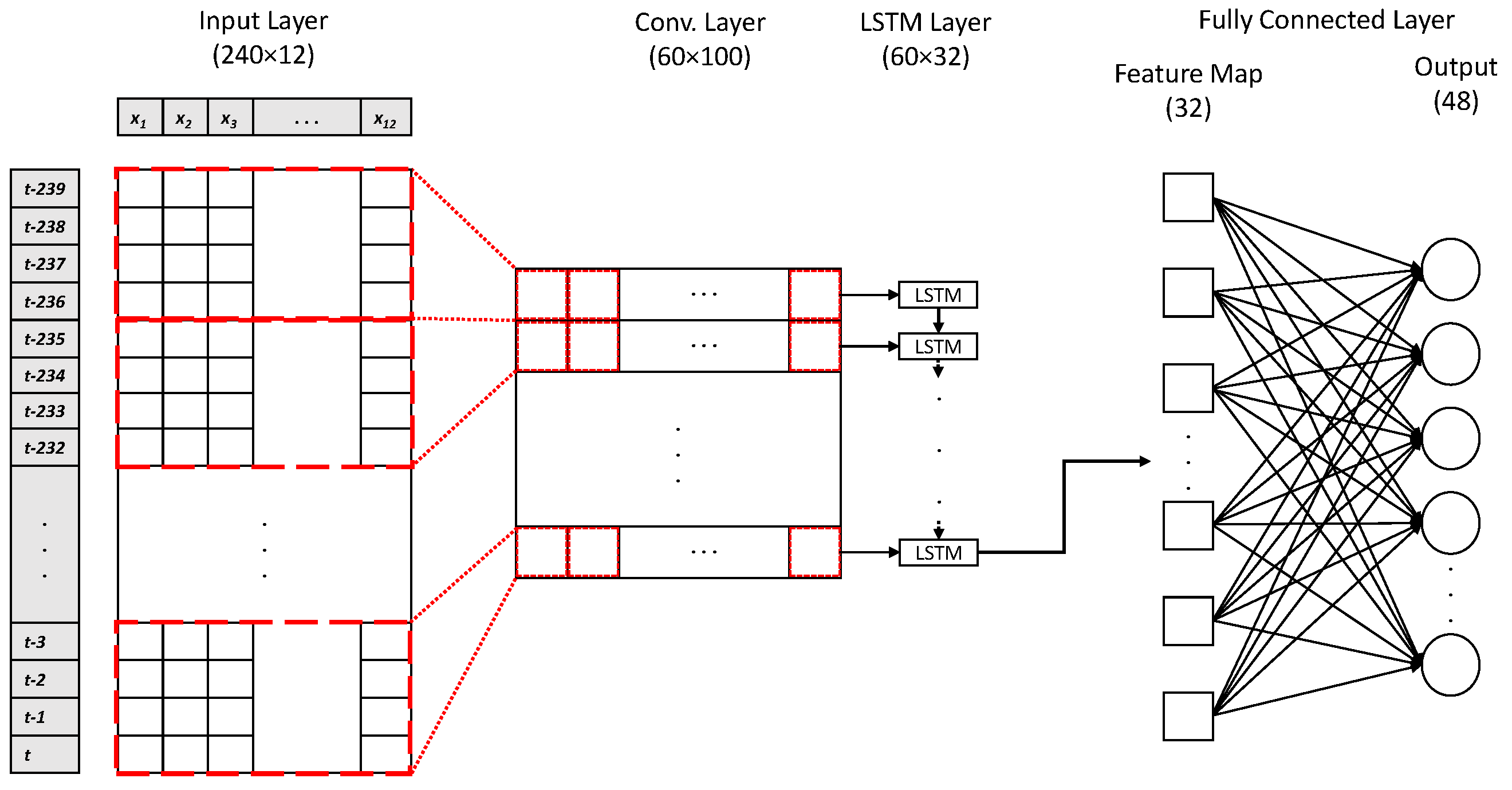
2.4.4. CNN-LSTM Model
2.5. Model Evaluation Metrics
2.6. Implementation Details
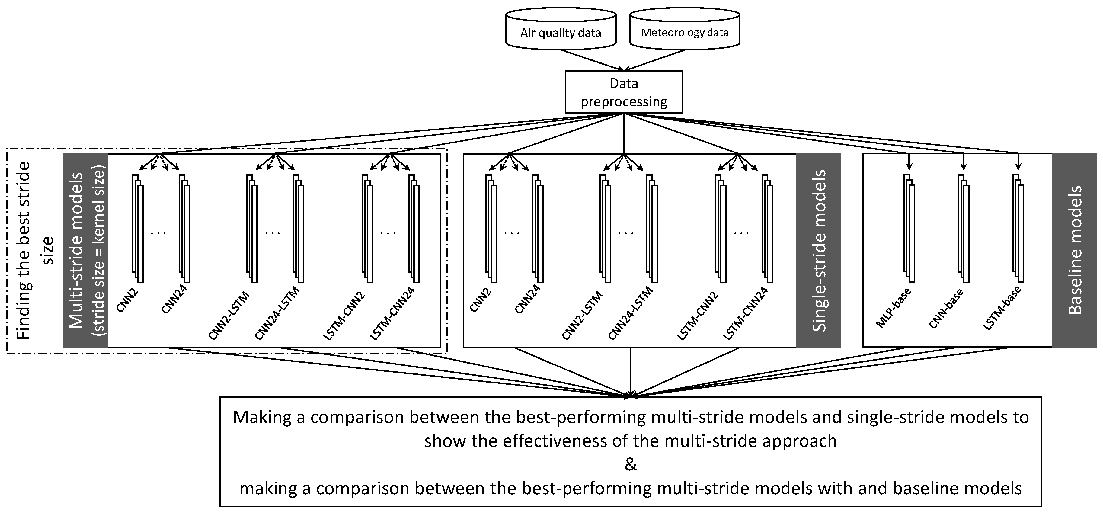
3. Experiments
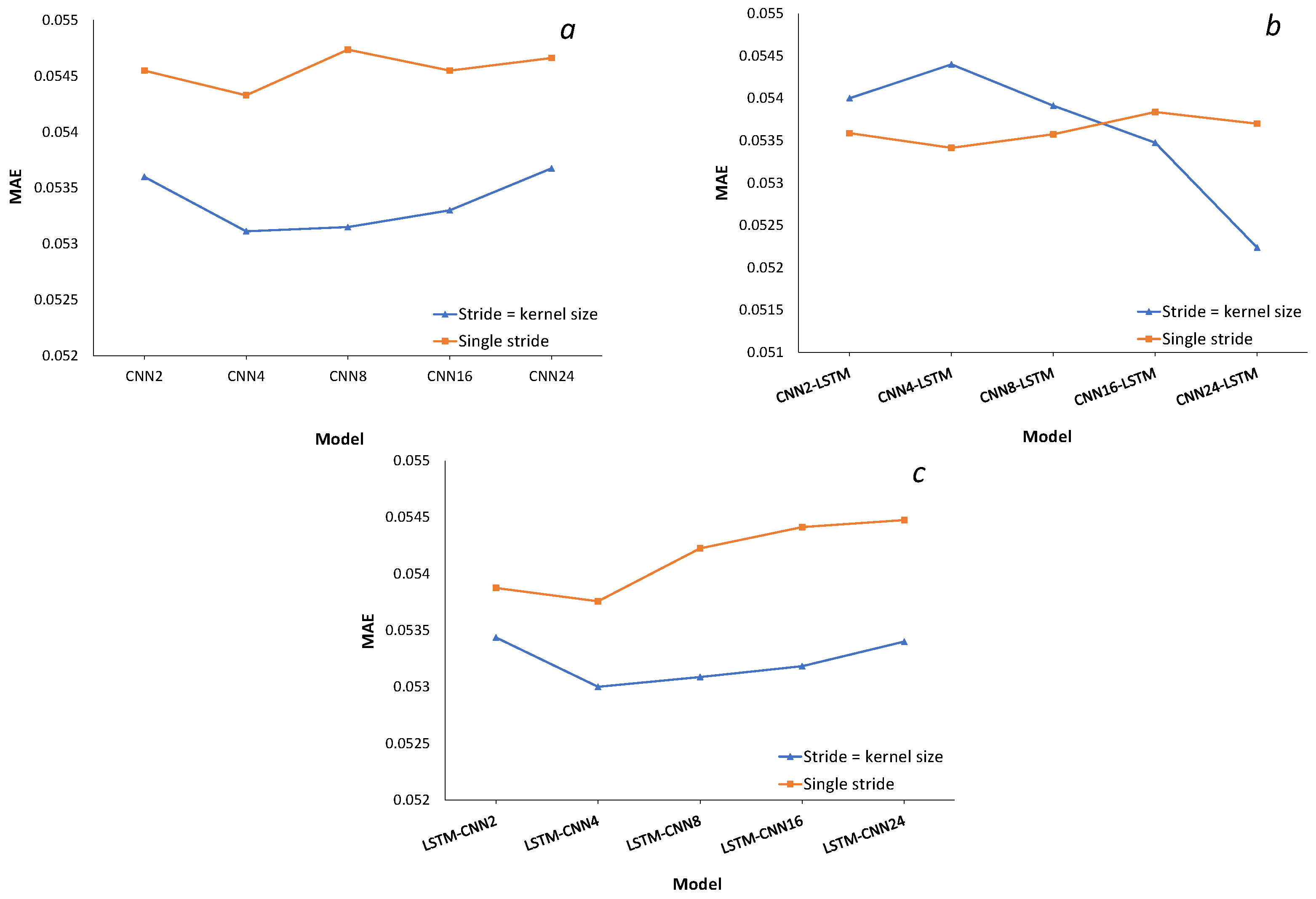
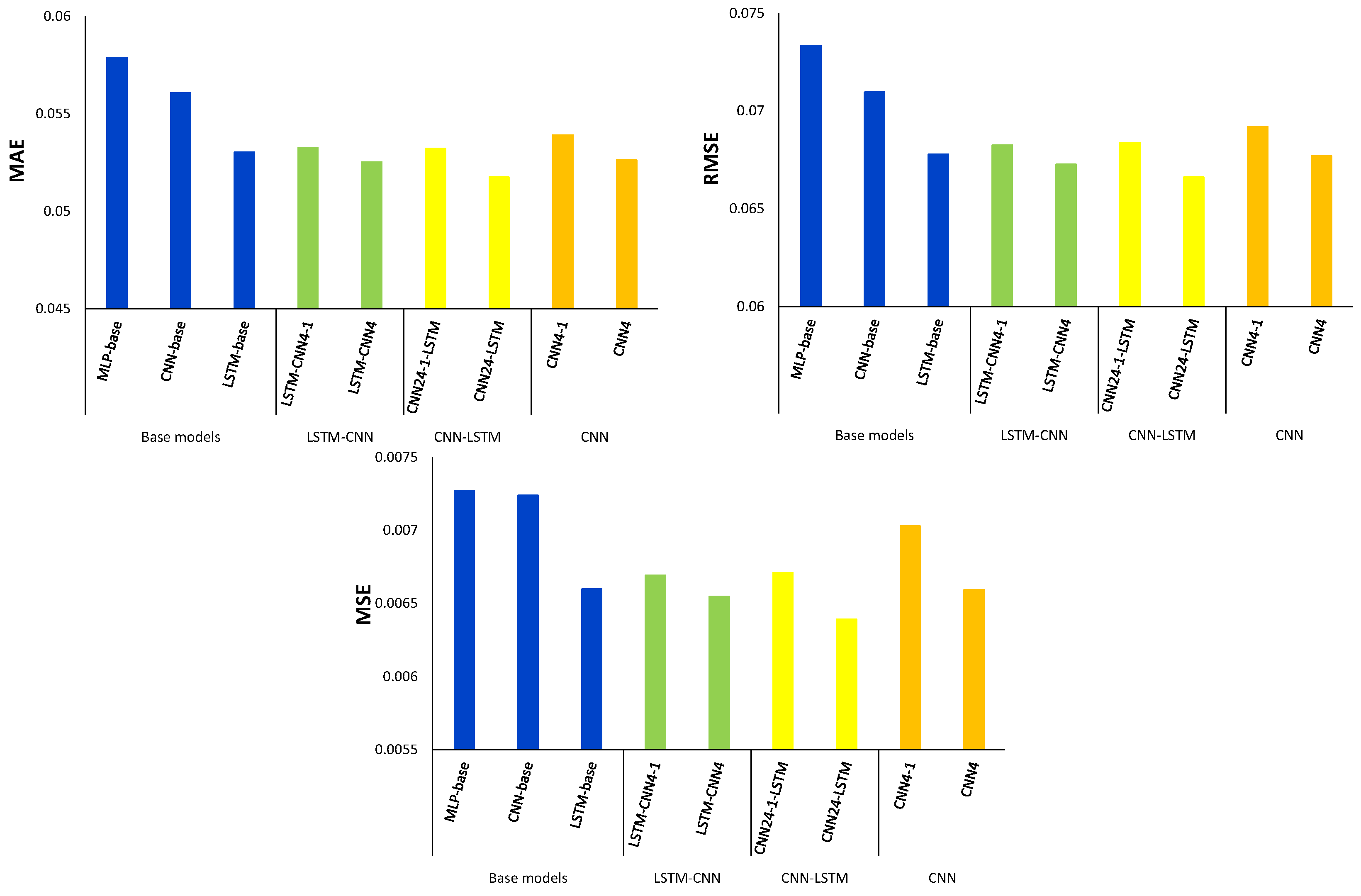
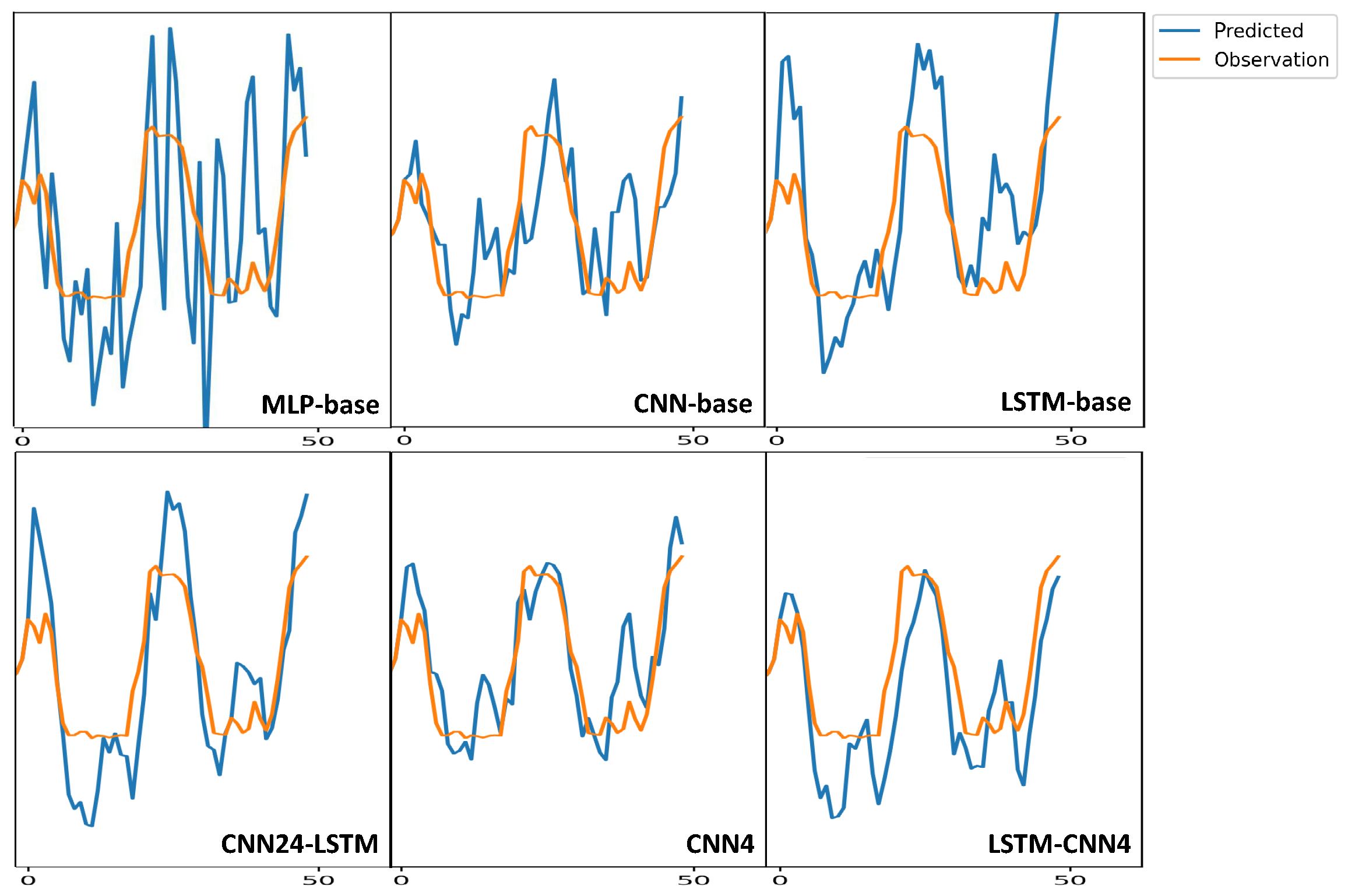
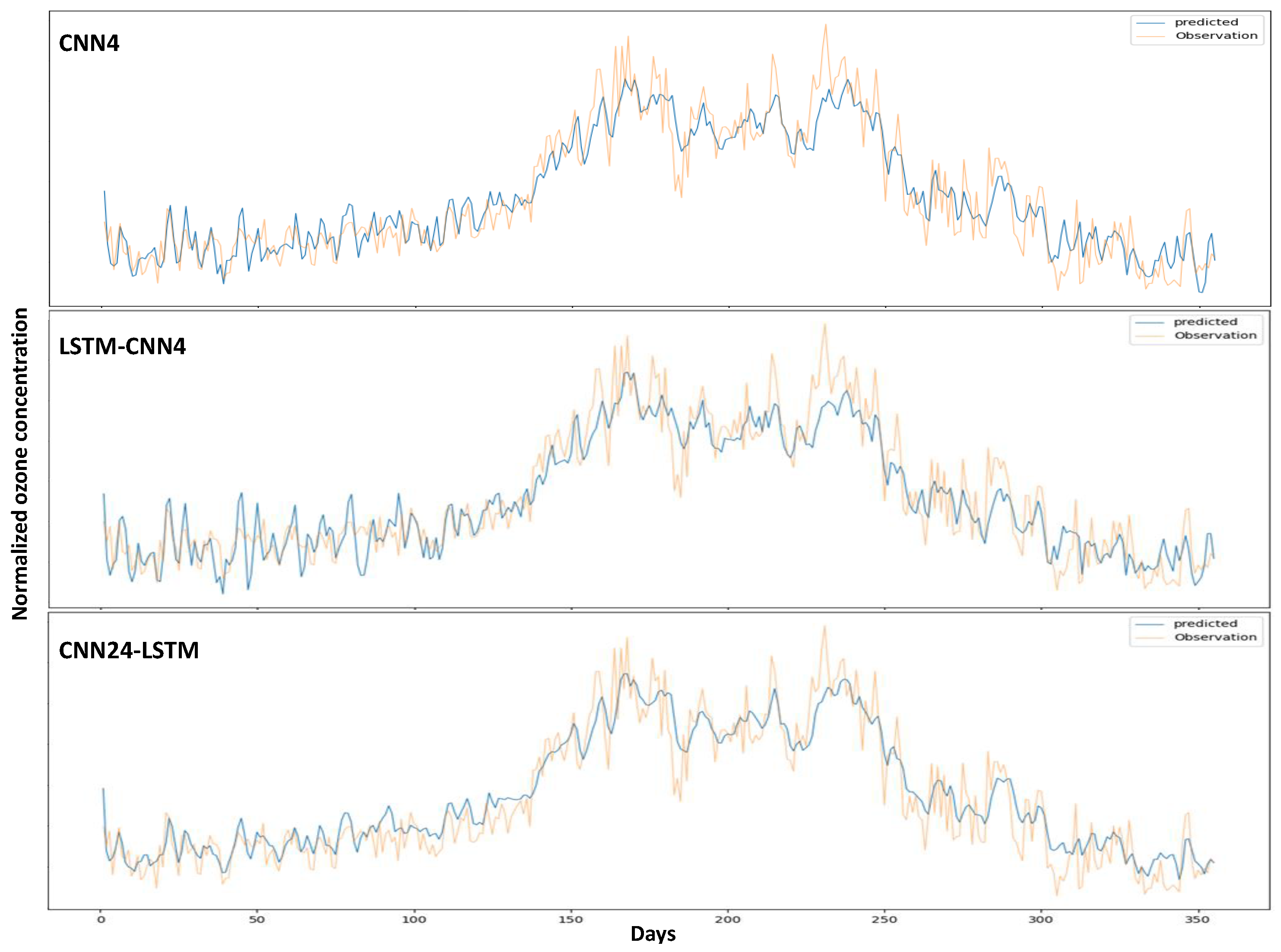
Empirical Results
4. Discussion
5. Conclusions
Author Contributions
Funding
Institutional Review Board Statement
Informed Consent Statement
Data Availability Statement
Conflicts of Interest
Abbreviations
| CMAQ | Community Multiscale Air Quality modeling system |
| CNN | Convolutional Neural Network |
| LSTM | Long Short-Term Memory |
| MAE | Mean Absolute Error |
| MLP | Multilayer Perceptron |
| MSE | Mean Square Error |
| RMSE | Root Mean Square Error |
| RNN | Recurrent Neural Network |
| STE | Stratosphere-to-Troposphere Exchanges |
| VOCs | Volatile Organic Compounds |
| WRF | Weather Research and Forecasting model |
References
- Fleming, Z.L.; Doherty, R.M.; Von Schneidemesser, E.; Malley, C.; Cooper, O.R.; Pinto, J.P.; Colette, A.; Xu, X.; Simpson, D.; Schultz, M.G.; et al. Tropospheric Ozone Assessment Report: Present-day ozone distribution and trends relevant to human health. Elem. Sci. Anthr. 2018, 6. [Google Scholar] [CrossRef] [Green Version]
- Feng, Z.; De Marco, A.; Anav, A.; Gualtieri, M.; Sicard, P.; Tian, H.; Fornasier, F.; Tao, F.; Guo, A.; Paoletti, E. Economic losses due to ozone impacts on human health, forest productivity and crop yield across China. Environ. Int. 2019, 131, 104966. [Google Scholar] [CrossRef] [PubMed]
- Kim, Y.; Choi, Y.H.; Kim, M.K.; Paik, H.J.; Kim, D.H. Different adverse effects of air pollutants on dry eye disease: Ozone, PM2.5, and PM10. Environ. Pollut. 2020, 265, 115039. [Google Scholar] [CrossRef]
- Maji, K.J.; Namdeo, A. Continuous increases of surface ozone and associated premature mortality growth in China during 2015–2019. Environ. Pollut. 2021, 269, 116183. [Google Scholar] [CrossRef] [PubMed]
- Silva, R.A.; West, J.J.; Zhang, Y.; Anenberg, S.C.; Lamarque, J.F.; Shindell, D.T.; Collins, W.J.; Dalsoren, S.; Faluvegi, G.; Folberth, G.; et al. Global premature mortality due to anthropogenic outdoor air pollution and the contribution of past climate change. Environ. Res. Lett. 2013, 8, 034005. [Google Scholar] [CrossRef]
- Tiwari, S.; Agrawal, M. Tropospheric Ozone and Its Impacts on Crop Plants; Springer: Delhi, India, 2018; p. 201. [Google Scholar]
- Škerlak, B.; Sprenger, M.; Wernli, H. A global climatology of stratosphere-troposphere exchange using the ERA-Interim data set from 1979 to 2011. Atmos. Chem. Phys. 2014, 14, 913–937. [Google Scholar] [CrossRef] [Green Version]
- Hofmann, C.; Kerkweg, A.; Hoor, P.; Jöckel, P. Stratosphere-troposphere exchange in the vicinity of a tropopause fold. Atmos. Chem. Phys. Discuss. 2016, 1–26. [Google Scholar] [CrossRef] [Green Version]
- Revell, L.E.; Tummon, F.; Stenke, A.; Sukhodolov, T.; Coulon, A.; Rozanov, E.; Garny, H.; Grewe, V.; Peter, T. Drivers of the tropospheric ozone budget throughout the 21st century under the medium-high climate scenario RCP 6.0. Atmos. Chem. Phys. 2015, 15, 5887–5902. [Google Scholar] [CrossRef] [Green Version]
- Jacob, D.J. Introduction to Atmospheric Chemistry, 11th ed.; Princeton University Press: Princeton, NJ, USA, 1999; p. 280. [Google Scholar]
- Monks, P.S.; Archibald, A.; Colette, A.; Cooper, O.; Coyle, M.; Derwent, R.; Fowler, D.; Granier, C.; Law, K.S.; Mills, G.; et al. Tropospheric ozone and its precursors from the urban to the global scale from air quality to short-lived climate forcer. Atmos. Chem. Phys. 2015, 15, 8889–8973. [Google Scholar] [CrossRef] [Green Version]
- Kim, S.; VandenBoer, T.C.; Young, C.J.; Riedel, T.P.; Thornton, J.A.; Swarthout, B.; Sive, B.; Lerner, B.; Gilman, J.B.; Warneke, C.; et al. The primary and recycling sources of OH during the NACHTT-2011 campaign: HONO as an important OH primary source in the wintertime. J. Geophys. Res. Atmos. 2014, 119, 6886–6896. [Google Scholar] [CrossRef] [Green Version]
- Fiore, A.M.; Naik, V.; Leibensperger, E.M. Air quality and climate connections. J. Air Waste Manag. Assoc. 2015, 65, 645–685. [Google Scholar] [CrossRef]
- Oswald, E.M.; Dupigny-Giroux, L.A.; Leibensperger, E.M.; Poirot, R.; Merrell, J. Climate controls on air quality in the Northeastern US: An examination of summertime ozone statistics during 1993–2012. Atmos. Environ. 2015, 112, 278–288. [Google Scholar] [CrossRef] [Green Version]
- Lefohn, A.S.; Malley, C.S.; Smith, L.; Wells, B.; Hazucha, M.; Simon, H.; Naik, V.; Mills, G.; Schultz, M.G.; Paoletti, E.; et al. Tropospheric ozone assessment report: Global ozone metrics for climate change, human health, and crop/ecosystem research. Elementa 2018, 1, 1. [Google Scholar] [CrossRef] [PubMed] [Green Version]
- Fowler, D.; Amann, M.; Anderson, R.; Ashmore, M.; Cox, P.; Depledge, M.; Derwent, D.; Grennfelt, P.; Hewitt, N.; Hov, O.; et al. Ground-Level Ozone in the 21st Century: Future Trends, Impacts and Policy Implications; The Royal Society: London, UK, 2008; Volume 15/08. [Google Scholar]
- Jacob, D.J.; Winner, D.A. Effect of climate change on air quality. Atmos. Environ. 2009, 43, 51–63. [Google Scholar] [CrossRef] [Green Version]
- Itahashi, S.; Hayami, H.; Uno, I. Comprehensive study of emission source contributions for tropospheric ozone formation over East Asia. J. Geophys. Res. Atmos. 2015, 120, 331–358. [Google Scholar] [CrossRef]
- Yi, X.; Zhang, J.; Wang, Z.; Li, T.; Zheng, Y. Deep distributed fusion network for air quality prediction. In Proceedings of the 24th ACM SIGKDD International Conference on Knowledge Discovery & Data Mining, London, UK, 19–23 August 2018; pp. 965–973. [Google Scholar]
- Wang, J.; Song, G. A deep spatial-temporal ensemble model for air quality prediction. Neurocomputing 2018, 314, 198–206. [Google Scholar] [CrossRef]
- Li, X.; Peng, L.; Hu, Y.; Shao, J.; Chi, T. Deep learning architecture for air quality predictions. Environ. Sci. Pollut. Res. 2016, 23, 22408–22417. [Google Scholar] [CrossRef]
- Wang, H.W.; Li, X.B.; Wang, D.; Zhao, J.; Peng, Z.R. Regional prediction of ground-level ozone using a hybrid sequence-to-sequence deep learning approach. J. Clean. Prod. 2020, 253, 119841. [Google Scholar] [CrossRef]
- Gradišar, D.; Grašič, B.; Božnar, M.Z.; Mlakar, P.; Kocijan, J. Improving of local ozone forecasting by integrated models. Environ. Sci. Pollut. Res. 2016, 23, 18439–18450. [Google Scholar] [CrossRef]
- Feng, R.; Zheng, H.J.; Zhang, A.R.; Huang, C.; Gao, H.; Ma, Y.C. Unveiling tropospheric ozone by the traditional atmospheric model and machine learning, and their comparison: A case study in Hangzhou, China. Environ. Pollut. 2019, 252, 366–378. [Google Scholar] [CrossRef]
- Jia, P.; Cao, N.; Yang, S. Real-time hourly ozone prediction system for Yangtze River Delta area using attention based on a sequence to sequence model. Atmos. Environ. 2021, 244, 117917. [Google Scholar] [CrossRef]
- Mekparyup, J.; Saithanu, K. Application of Artificial Neural Network Models to Predict the Ozone Concentration at the East of Thailand. Int. J. Appl. Environ. Sci. 2014, 9, 1291–1296. [Google Scholar]
- Hoffman, S.; Jasiński, R. The Use of Multilayer Perceptrons to Model PM2.5 Concentrations at Air Monitoring Stations in Poland. Atmosphere 2023, 14, 96. [Google Scholar] [CrossRef]
- Özbay, B.; Keskin, G.A.; Doğruparmak, Ş.Ç.; Ayberk, S. Predicting tropospheric ozone concentrations in different temporal scales by using multilayer perceptron models. Ecol. Inform. 2011, 6, 242–247. [Google Scholar]
- ALves, L.; Nascimento, E.G.S.; Moreira, D.M. Hourly tropospheric ozone concentration forecasting using deep learning. WIT Trans. Ecol. Environ. 2019, 236, 129–138. [Google Scholar]
- Chattopadhyay, G.; Midya, S.K.; Chattopadhyay, S. MLP based predictive model for surface ozone concentration over an urban area in the Gangetic West Bengal during pre-monsoon season. J. Atmos. Sol.-Terr. Phys. 2019, 184, 57–62. [Google Scholar] [CrossRef]
- Hassan, M.A.; Dong, Z. Analysis of Tropospheric Ozone by Artificial Neural Network Approach in Beijing. J. Geosci. Environ. Prot. 2018, 6, 8–17. [Google Scholar] [CrossRef] [Green Version]
- Hijjawi, M.A.M.S.M. Ground-level Ozone Prediction Using Machine Learning Techniques: A Case Study in Amman, Jordan. Int. J. Autom. Comput. 2020, 17, 667–677. [Google Scholar]
- Deng, T.; Manders, A.; Jin, J.; Lin, H.X. Clustering-based spatial transfer learning for short-term ozone forecasting. J. Hazard. Mater. Adv. 2022, 8, 100168. [Google Scholar] [CrossRef]
- Song, Z.; Deng, Q.; Ren, Z. Correlation and principal component regression analysis for studying air quality and meteorological elements in Wuhan, China. Environ. Prog. Sustain. Energy 2020, 39, 13278. [Google Scholar] [CrossRef]
- Su, X.; An, J.; Zhang, Y.; Zhu, P.; Zhu, B. Prediction of ozone hourly concentrations by support vector machine and kernel extreme learning machine using wavelet transformation and partial least squares methods. Atmos. Pollut. Res. 2020, 11, 51–60. [Google Scholar] [CrossRef]
- Liu, B.C.; Binaykia, A.; Chang, P.C.; Tiwari, M.K.; Tsao, C.C. Urban air quality forecasting based on multi-dimensional collaborative Support Vector Regression (SVR): A case study of Beijing-Tianjin-Shijiazhuang. PLoS ONE 2017, 12, e0179763. [Google Scholar] [CrossRef] [PubMed] [Green Version]
- Sanchez-Torres, G.; Bolaño, I.D. Support Vector Regression for PM10 Concentration Modeling in Santa Marta Urban Area. Eng. Lett. 2019, 27, 432–440. [Google Scholar]
- Liu, H.; Li, Q.; Yu, D.; Gu, Y. Air quality index and air pollutant concentration prediction based on machine learning algorithms. Appl. Sci. 2019, 9, 4069. [Google Scholar] [CrossRef] [Green Version]
- Murillo-Escobar, J.; Sepulveda-Suescun, J.; Correa, M.; Orrego-Metaute, D. Forecasting concentrations of air pollutants using support vector regression improved with particle swarm optimization: Case study in Aburrá Valley, Colombia. Urban Clim. 2019, 29, 100473. [Google Scholar] [CrossRef]
- Castelli, M.; Clemente, F.M.; Popovič, A.; Silva, S.; Vanneschi, L. A Machine Learning Approach to Predict Air Quality in California. Complexity 2020, 2020, 8049504. [Google Scholar] [CrossRef]
- Jumin, E.; Zaini, N.; Ahmed, A.N.; Abdullah, S.; Ismail, M.; Sherif, M.; Sefelnasr, A.; El-Shafie, A. Machine learning versus linear regression modelling approach for accurate ozone concentrations prediction. Eng. Appl. Comput. Fluid Mech. 2020, 14, 713–725. [Google Scholar]
- Plocoste, T.; Laventure, S. Forecasting PM10 Concentrations in the Caribbean Area Using Machine Learning Models. Atmosphere 2023, 14, 134. [Google Scholar] [CrossRef]
- Pak, U.; Kim, C.; Ryu, U.; Sok, K.; Pak, S. A hybrid model based on convolutional neural networks and long short-term memory for ozone concentration prediction. Air Qual. Atmos. Health 2018, 11, 883–895. [Google Scholar] [CrossRef]
- Freeman, B.S.; Taylor, G.; Gharabaghi, B.; Thé, J. Forecasting air quality time series using deep learning. J. Air Waste Manag. Assoc. 2018, 68, 866–886. [Google Scholar] [CrossRef] [Green Version]
- Eslami, E.; Choi, Y.; Lops, Y.; Sayeed, A. A real-time hourly ozone prediction system using deep convolutional neural network. Neural Comput. Appl. 2019, 32, 8783–8797. [Google Scholar] [CrossRef] [Green Version]
- Sayeed, A.; Choi, Y.; Eslami, E.; Lops, Y.; Roy, A.; Jung, J. Using a deep convolutional neural network to predict 2017 ozone concentrations, 24 hours in advance. Neural Netw. 2020, 121, 396–408. [Google Scholar] [CrossRef]
- Khamparia, A.; Singh, K.M. A systematic review on deep learning architectures and applications. Expert Syst. 2019, 36, e12400. [Google Scholar] [CrossRef]
- Liu, D.R.; Lee, S.J.; Huang, Y.; Chiu, C.J. Air pollution forecasting based on attention-based LSTM neural network and ensemble learning. Expert Syst. 2020, 37, e12511. [Google Scholar] [CrossRef]
- Chang, Y.S.; Chiao, H.T.; Abimannan, S.; Huang, Y.P.; Tsai, Y.T.; Lin, K.M. An LSTM-based aggregated model for air pollution forecasting. Atmos. Pollut. Res. 2020, 11, 1451–1463. [Google Scholar] [CrossRef]
- Navares, R.; Aznarte, J.L. Predicting air quality with deep learning LSTM: Towards comprehensive models. Ecol. Inform. 2020, 55, 101019. [Google Scholar] [CrossRef]
- Zhang, L.; Liu, P.; Zhao, L.; Wang, G.; Zhang, W.; Liu, J. Air quality predictions with a semi-supervised bidirectional LSTM neural network. Atmos. Pollut. Res. 2021, 12, 328–339. [Google Scholar] [CrossRef]
- Nabavi, S.O.; Nölscher, A.C.; Samimi, C.; Thomas, C.; Haimberger, L.; Lüers, J.; Held, A. Site-scale modeling of surface ozone in Northern Bavaria using machine learning algorithms, regional dynamic models, and a hybrid model. Environ. Pollut. 2021, 268, 115736. [Google Scholar] [CrossRef]
- Dai, H.; Huang, G.; Zeng, H.; Yu, R. Haze Risk Assessment Based on Improved PCA-MEE and ISPO-LightGBM Model. Systems 2022, 10, 263. [Google Scholar] [CrossRef]
- Dai, H.; Huang, G.; Zeng, H.; Zhou, F. PM2.5 volatility prediction by XGBoost-MLP based on GARCH models. J. Clean. Prod. 2022, 356, 131898. [Google Scholar] [CrossRef]
- Sayeed, A.; Eslami, E.; Lops, Y.; Choi, Y. CMAQ-CNN: A new-generation of post-processing techniques for chemical transport models using deep neural networks. Atmos. Environ. 2022, 273, 118961. [Google Scholar] [CrossRef]
- Kim, H.S.; Han, K.M.; Yu, J.; Kim, J.; Kim, K.; Kim, H. Development of a CNN+ LSTM Hybrid Neural Network for Daily PM2.5 Prediction. Atmosphere 2022, 13, 2124. [Google Scholar] [CrossRef]
- Zhao, Q.; Jiang, K.; Talifu, D.; Gao, B.; Wang, X.; Abulizi, A.; Zhang, X.; Liu, B. Simulation of the Ozone Concentration in Three Regions of Xinjiang, China, Using a Genetic Algorithm-Optimized BP Neural Network Model. Atmosphere 2023, 14, 160. [Google Scholar] [CrossRef]
- Cirstea, R.G.; Micu, D.V.; Muresan, G.M.; Guo, C.; Yang, B. Correlated time series forecasting using multi-task deep neural networks. In Proceedings of the 27th ACM International Conference on Information and Knowledge Management, Torino, Italy, 22–26 October 2018; pp. 1527–1530. [Google Scholar]
- National Research Council. Rethinking the Ozone Problem in Urban and Regional Air Pollution; National Academies Press: Washington, DC, USA, 1992. [Google Scholar]
- Li, Y.; Yu, R.; Shahabi, C.; Liu, Y. Diffusion convolutional recurrent neural network: Data-driven traffic forecasting. arXiv 2017, arXiv:1707.01926. [Google Scholar]
- Ait-Amir, B.; Pougnet, P.; El Hami, A. Embedded Mechatronic Systems 2; Elsevier: Amsterdam, The Netherlands, 2015; pp. 151–179. [Google Scholar]
- Chai, T.; Draxler, R.R. Root mean square error (RMSE) or mean absolute error (MAE)? Geosci. Model Dev. 2014, 7, 1525–1534. [Google Scholar] [CrossRef] [Green Version]
- Srivastava, N.; Hinton, G.; Krizhevsky, A.; Sutskever, I.; Salakhutdinov, R. Dropout: A simple way to prevent neural networks from overfitting. J. Mach. Learn. Res. 2014, 15, 1929–1958. [Google Scholar]
- Mehdipour, V.; Memarianfard, M. Application of support vector machine and gene expression programming on tropospheric ozone prognosticating for Tehran metropolitan. Civ. Eng. J. 2017, 3, 557–567. [Google Scholar] [CrossRef]


| Station | Station | ||||||||
|---|---|---|---|---|---|---|---|---|---|
| Alibeyköy | Mean | 45.583 | 100.627 | 22.802 | Başakşehir | Mean | 31.681 | 56.149 | 55.013 |
| Std. | 30.603 | 134.910 | 23.088 | Std. | 25.632 | 70.125 | 28.306 | ||
| Q1 * | 25.900 | 30.400 | 4.000 | Q1 | 14.376 | 19.265 | 34.245 | ||
| Q2 | 39.000 | 56.400 | 15.400 | Q2 | 23.740 | 33.124 | 57.900 | ||
| Q3 | 57.290 | 109.900 | 34.200 | Q3 | 40.734 | 60.993 | 75.680 | ||
| Miss. (%) ** | 14.13 | Miss. (%) | 5.85 | ||||||
| Beşiktaş | Mean | 73.898 | 182.003 | 27.330 | Esenyurt | Mean | 25.762 | 88.345 | 35.030 |
| Std. | 35.057 | 127.797 | 17.759 | Std. | 17.922 | 116.479 | 26.203 | ||
| Q1 | 48.600 | 88.900 | 12.900 | Q1 | 12.850 | 30.631 | 13.743 | ||
| Q2 | 68.200 | 145.869 | 24.000 | Q2 | 21.250 | 53.107 | 32.100 | ||
| Q3 | 92.588 | 241.900 | 39.000 | Q3 | 34.335 | 93.976 | 51.130 | ||
| Miss. (%) | 7.67 | Miss. (%) | 5.45 | ||||||
| Kadıköy | Mean | 56.129 | 153.261 | 20.158 | Kağıthane | Mean | 36.530 | 101.051 | 44.949 |
| Std. | 31.364 | 224.346 | 14.927 | Std. | 28.642 | 120.980 | 30.859 | ||
| Q1 | 35.800 | 49.500 | 9.600 | Q1 | 16.670 | 37.239 | 20.650 | ||
| Q2 | 49.434 | 85.900 | 16.200 | Q2 | 28.901 | 62.552 | 42.500 | ||
| Q3 | 68.800 | 156.100 | 28.600 | Q3 | 48.630 | 115.374 | 65.872 | ||
| Miss. (%) | 7.36 | Miss. (%) | 4.27 | ||||||
| Sultanbeyli | Mean | 19.497 | 45.148 | 58.245 | Sultangazi | Mean | 35.068 | 75.146 | 35.329 |
| Std. | 20.942 | 75.336 | 33.931 | Std. | 22.142 | 81.717 | 23.783 | ||
| Q1 | 4.802 | 8.059 | 30.800 | Q1 | 20.610 | 33.527 | 14.390 | ||
| Q2 | 10.819 | 17.473 | 61.600 | Q2 | 30.925 | 55.171 | 34.050 | ||
| Q3 | 27.755 | 47.033 | 83.700 | Q3 | 44.690 | 88.654 | 52.941 | ||
| Miss. (%) | 3.15 | Miss. (%) | 3.69 | ||||||
| Station | Parameter | Mean | Std. | Q1 | Q2 | Q3 | Miss. (%) |
|---|---|---|---|---|---|---|---|
| Güngören D. | Pressure (hPa) | 1008.30 | 6.55 | 1003.90 | 1007.80 | 1012.50 | 3.27 |
| R. humidity (%) | 72.72 | 15.68 | 62.00 | 74.00 | 85.00 | ||
| Temperature (C) | 15.89 | 7.78 | 9.60 | 15.90 | 22.40 | ||
| Precipitation (mm) | 0.12 | 1.06 | 0.00 | 0.00 | 0.00 | ||
| Wind speed (ms) | 3.21 | 1.64 | 1.90 | 3.00 | 4.20 | ||
| Solar rad. (Wm) | 9806.21 | 15,195.13 | 0.00 | 0.00 | 15,600.00 | ||
| Kadıköy R. | Pressure (hPa) | 1014.69 | 6.67 | 1010.10 | 1014.10 | 1018.90 | 3.27 |
| R. humidity (%) | 73.02 | 13.59 | 64.00 | 74.00 | 83.00 | ||
| Temperature(C) | 16.40 | 7.59 | 10.20 | 16.30 | 22.60 | ||
| Precipitation(mm) | 0.08 | 0.59 | 0.00 | 0.00 | 0.00 | ||
| Wind speed (ms) | 3.27 | 1.83 | 1.80 | 2.90 | 4.40 | ||
| Şişli | R. humidity (%) | 73.00 | 17.60 | 61.00 | 74.00 | 87.00 | 3.71 |
| Temperature(C) | 16.09 | 7.67 | 9.80 | 16.20 | 22.50 | ||
| Precipitation (mm) | 0.09 | 0.61 | 0.00 | 0.00 | 0.00 | ||
| Wind speed (ms) | 1.96 | 0.96 | 1.30 | 1.90 | 2.60 | ||
| Sancaktepe | Temperature(C) | 14.77 | 8.05 | 8.20 | 14.90 | 21.00 | 2.92 |
| Precipitation(mm) | 0.10 | 0.70 | 0.00 | 0.00 | 0.00 | ||
| Wind speed (ms) | 2.52 | 1.72 | 1.10 | 2.20 | 3.60 | ||
| Samandıra H. | Pressure (hPa) | 1002.11 | 6.77 | 997.50 | 1001.50 | 1006.40 | 4.13 |
| R. humidity (%) | 77.45 | 17.27 | 65.00 | 81.00 | 92.00 |
| Models | Jan | Feb | Mar | Apr | May | Jun | Jul | Aug | Sep | Oct | Nov | Dec | |
|---|---|---|---|---|---|---|---|---|---|---|---|---|---|
| MSE | MLP-base | 0.0063 | 0.0085 | 0.0102 | 0.0113 | 0.0111 | 0.0078 | 0.0064 | 0.0058 | 0.0070 | 0.0043 | 0.0050 | 0.0036 |
| CNN-base | 0.0061 | 0.0089 | 0.0108 | 0.0113 | 0.0110 | 0.0078 | 0.0062 | 0.0063 | 0.0066 | 0.0041 | 0.0045 | 0.0033 | |
| LSTM-base | 0.0059 | 0.0073 | 0.0095 | 0.0103 | 0.0099 | 0.0069 | 0.0052 | 0.0053 | 0.0074 | 0.0043 | 0.0042 | 0.0031 | |
| LSTM-CNN4-1 | 0.0060 | 0.0078 | 0.0100 | 0.0107 | 0.0104 | 0.0071 | 0.0054 | 0.0052 | 0.0064 | 0.0037 | 0.0044 | 0.0032 | |
| LSTM-CNN4 | 0.0060 | 0.0073 | 0.0100 | 0.0106 | 0.0102 | 0.0069 | 0.0052 | 0.0050 | 0.0064 | 0.0036 | 0.0043 | 0.0031 | |
| CNN24-1-LSTM | 0.0061 | 0.0073 | 0.0094 | 0.0108 | 0.0103 | 0.0070 | 0.0056 | 0.0054 | 0.0069 | 0.0041 | 0.0045 | 0.0032 | |
| CNN24-LSTM | 0.0058 | 0.0070 | 0.0092 | 0.0102 | 0.0098 | 0.0068 | 0.0054 | 0.0052 | 0.0066 | 0.0039 | 0.0040 | 0.0029 | |
| CNN4-1 | 0.0065 | 0.0084 | 0.0097 | 0.0115 | 0.0108 | 0.0069 | 0.0056 | 0.0053 | 0.0071 | 0.0041 | 0.0050 | 0.0035 | |
| CNN4 | 0.0059 | 0.0077 | 0.0095 | 0.0106 | 0.0104 | 0.0070 | 0.0055 | 0.0052 | 0.0065 | 0.0038 | 0.0044 | 0.0028 | |
| RMSE | MLP-base | 0.0673 | 0.0799 | 0.0882 | 0.0938 | 0.0910 | 0.0773 | 0.0721 | 0.0682 | 0.0705 | 0.0581 | 0.0609 | 0.0530 |
| CNN-base | 0.0646 | 0.0801 | 0.0890 | 0.0921 | 0.0881 | 0.0750 | 0.0682 | 0.0689 | 0.0666 | 0.0549 | 0.0562 | 0.0482 | |
| LSTM-base | 0.0635 | 0.0728 | 0.0835 | 0.0879 | 0.0844 | 0.0711 | 0.0629 | 0.0648 | 0.0692 | 0.0556 | 0.0535 | 0.0445 | |
| LSTM-CNN4-1 | 0.0634 | 0.0751 | 0.0862 | 0.0895 | 0.0860 | 0.0718 | 0.0638 | 0.0639 | 0.0653 | 0.0522 | 0.0552 | 0.0469 | |
| LSTM-CNN4 | 0.0632 | 0.0730 | 0.0856 | 0.0890 | 0.0845 | 0.0706 | 0.0626 | 0.0627 | 0.0648 | 0.0516 | 0.0543 | 0.0455 | |
| CNN24-1-LSTM | 0.0642 | 0.0729 | 0.0829 | 0.0898 | 0.0856 | 0.0713 | 0.0652 | 0.0650 | 0.0681 | 0.0545 | 0.0551 | 0.0459 | |
| CNN24-LSTM | 0.0625 | 0.0718 | 0.0822 | 0.0874 | 0.0831 | 0.0703 | 0.0633 | 0.0638 | 0.0659 | 0.0535 | 0.0520 | 0.0438 | |
| CNN4-1 | 0.0650 | 0.0764 | 0.0828 | 0.0924 | 0.0856 | 0.0686 | 0.0639 | 0.0636 | 0.0685 | 0.0551 | 0.0588 | 0.0497 | |
| CNN4 | 0.0632 | 0.0747 | 0.0835 | 0.0892 | 0.0855 | 0.0712 | 0.0643 | 0.0633 | 0.0657 | 0.0529 | 0.0548 | 0.0441 | |
| MAE | MLP-base | 0.0539 | 0.0648 | 0.0713 | 0.0737 | 0.0727 | 0.0596 | 0.0561 | 0.0522 | 0.0561 | 0.0451 | 0.0477 | 0.0414 |
| CNN-base | 0.0513 | 0.0649 | 0.0731 | 0.0718 | 0.0705 | 0.0585 | 0.0534 | 0.0531 | 0.0531 | 0.0425 | 0.0439 | 0.0371 | |
| LSTM-base | 0.0494 | 0.0577 | 0.0670 | 0.0686 | 0.0672 | 0.0542 | 0.0485 | 0.0493 | 0.0543 | 0.0431 | 0.0420 | 0.0351 | |
| LSTM-CNN4-1 | 0.0502 | 0.0601 | 0.0689 | 0.0695 | 0.0686 | 0.0551 | 0.0489 | 0.0480 | 0.0514 | 0.0397 | 0.0432 | 0.0357 | |
| LSTM-CNN4 | 0.0498 | 0.0585 | 0.0688 | 0.0691 | 0.0677 | 0.0539 | 0.0482 | 0.0470 | 0.0512 | 0.0393 | 0.0424 | 0.0345 | |
| CNN24-1-LSTM | 0.0502 | 0.0577 | 0.0663 | 0.0698 | 0.0678 | 0.0541 | 0.0500 | 0.0491 | 0.0530 | 0.0414 | 0.0429 | 0.0365 | |
| CNN24-LSTM | 0.0494 | 0.0572 | 0.0649 | 0.0678 | 0.0658 | 0.0533 | 0.0482 | 0.0478 | 0.0515 | 0.0406 | 0.0407 | 0.0340 | |
| CNN4-1 | 0.0519 | 0.0615 | 0.0661 | 0.0716 | 0.0685 | 0.0523 | 0.0485 | 0.0470 | 0.0536 | 0.0419 | 0.0457 | 0.0385 | |
| CNN4 | 0.0498 | 0.0596 | 0.0667 | 0.0694 | 0.0681 | 0.0539 | 0.0490 | 0.0472 | 0.0518 | 0.0400 | 0.0425 | 0.0337 |
| Models | MLP-Base | CNN-Base | LSTM-Base | LSTM-CNN4-1 | LSTM-CNN4 | CNN24-1-LSTM | CNN24-LSTM | CNN4-1 | |
|---|---|---|---|---|---|---|---|---|---|
| MSE | CNN-base | 0.7692 | |||||||
| LSTM-base | 0.0006 | 0.0078 | |||||||
| LSTM-CNN4-1 | 0.0000 | 0.0003 | 0.4847 | ||||||
| LSTM-CNN4 | 0.0000 | 0.0003 | 0.6821 | 0.0030 | |||||
| CNN24-1-LSTM | 0.0001 | 0.0103 | 0.2080 | 0.8447 | 0.0987 | ||||
| CNN24-LSTM | 0.0000 | 0.0003 | 0.0083 | 0.0099 | 0.1265 | 0.0000 | |||
| CNN4-1 | 0.0482 | 0.2517 | 0.0141 | 0.0072 | 0.0012 | 0.0118 | 0.0006 | ||
| CNN4 | 0.0000 | 0.0002 | 0.9655 | 0.0703 | 0.5359 | 0.1233 | 0.0284 | 0.0006 | |
| RMSE | CNN-base | 0.0017 | |||||||
| LSTM-base | 0.0000 | 0.0021 | |||||||
| LSTM-CNN4-1 | 0.0000 | 0.0001 | 0.4757 | ||||||
| LSTM-CNN4 | 0.0000 | 0.0000 | 0.3834 | 0.0000 | |||||
| CNN24-1-LSTM | 0.0000 | 0.0037 | 0.1055 | 0.8204 | 0.0362 | ||||
| CNN24-LSTM | 0.0000 | 0.0000 | 0.0008 | 0.0067 | 0.1792 | 0.0000 | |||
| CNN4-1 | 0.0001 | 0.0915 | 0.0973 | 0.2032 | 0.0169 | 0.2170 | 0.0055 | ||
| CNN4 | 0.0000 | 0.0000 | 0.8485 | 0.1020 | 0.2233 | 0.0697 | 0.0103 | 0.0454 | |
| MAE | CNN-base | 0.0068 | |||||||
| LSTM-base | 0.0000 | 0.0013 | |||||||
| LSTM-CNN4-1 | 0.0000 | 0.0001 | 0.6583 | ||||||
| LSTM-CNN4 | 0.0000 | 0.0000 | 0.3091 | 0.0001 | |||||
| CNN24-1-LSTM | 0.0000 | 0.0015 | 0.5357 | 0.9095 | 0.1048 | ||||
| CNN24-LSTM | 0.0000 | 0.0000 | 0.0002 | 0.0035 | 0.0827 | 0.0000 | |||
| CNN4-1 | 0.0000 | 0.0408 | 0.2149 | 0.2961 | 0.0384 | 0.2233 | 0.0036 | ||
| CNN4 | 0.0000 | 0.0000 | 0.3876 | 0.0229 | 0.6471 | 0.1203 | 0.0174 | 0.0349 |
Disclaimer/Publisher’s Note: The statements, opinions and data contained in all publications are solely those of the individual author(s) and contributor(s) and not of MDPI and/or the editor(s). MDPI and/or the editor(s) disclaim responsibility for any injury to people or property resulting from any ideas, methods, instructions or products referred to in the content. |
© 2023 by the authors. Licensee MDPI, Basel, Switzerland. This article is an open access article distributed under the terms and conditions of the Creative Commons Attribution (CC BY) license (https://creativecommons.org/licenses/by/4.0/).
Share and Cite
Rezaei, R.; Naderalvojoud, B.; Güllü, G. A Comparative Study of Deep Learning Models on Tropospheric Ozone Forecasting Using Feature Engineering Approach. Atmosphere 2023, 14, 239. https://doi.org/10.3390/atmos14020239
Rezaei R, Naderalvojoud B, Güllü G. A Comparative Study of Deep Learning Models on Tropospheric Ozone Forecasting Using Feature Engineering Approach. Atmosphere. 2023; 14(2):239. https://doi.org/10.3390/atmos14020239
Chicago/Turabian StyleRezaei, Reza, Behzad Naderalvojoud, and Gülen Güllü. 2023. "A Comparative Study of Deep Learning Models on Tropospheric Ozone Forecasting Using Feature Engineering Approach" Atmosphere 14, no. 2: 239. https://doi.org/10.3390/atmos14020239