Numerical Simulation of Wind Characteristics in Complex Mountains with Focus on Terrain Boundary Transition Curve

Abstract

In recent years, an increasing number of projects have been developed in complex mountainous areas. The wind environment in mountainous areas, extremely complex due to the undulating terrain and diverse landscapes, is a key factor threatening the structural safety of buildings and their appurtenances in mountainous areas. Therefore, it is important to study the wind environment in complex terrain to clarify the wind resistance of structures in mountainous areas. Computational fluid dynamics (CFD) approaches are commonly used to examine wind fields in complex terrain; however, due to the limited range of terrain considered, direct modeling using terrain elevation data can result in truncated elevation differences, affecting the accuracy of numerical simulations. To address the problem of truncated elevation differences at terrain boundaries, the parameters of the wind tunnel contraction curve are optimized regarding the wind tunnel contraction section design principle. Moreover, several transition curves are analyzed and evaluated by numerical simulation methods, and a transition curve applicable to the terrain boundary transition form is proposed. The proposed terrain transition curves are applied to model the terrain of complex mountainous ski resort areas to be used in CFD numerical simulations. Furthermore, the accuracy of the numerical simulation is verified through a comparison with the field-measured data. Results indicate that the proposed method can accurately and effectively reflect the wind environment characteristics of a ski resort area. The proposed terrain transition curve provides a theoretical basis and case support for designing the terrain model boundary transition section, which can be used as a reference for wind tunnel and numerical simulation studies in complex mountainous areas.

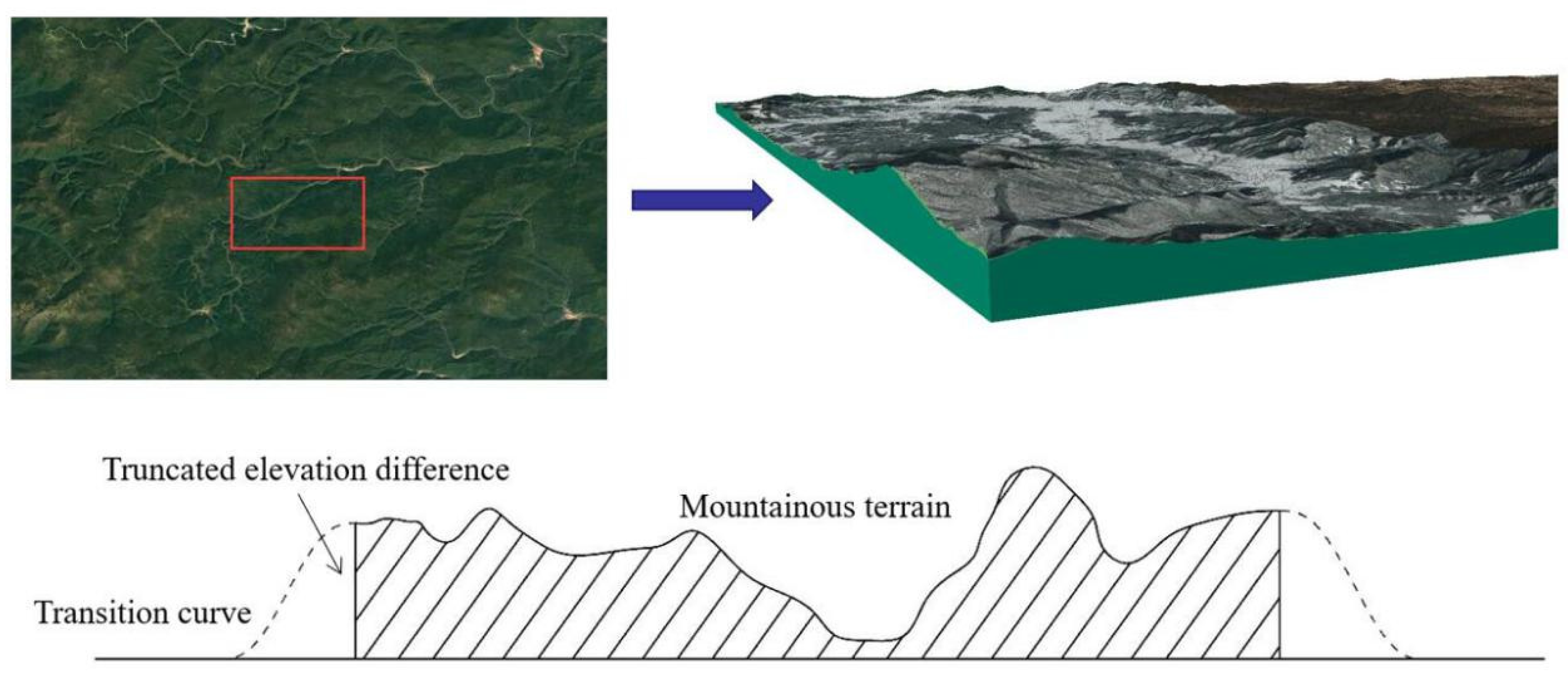
1. Introduction

With the rapid development of infrastructure, such as transportation and construction, an increasing number of development projects are being implemented in complex mountainous areas. Due to the undulating nature of the terrain, complex geological conditions, and the presence of diverse landforms in complex mountainous areas, the wind environment is affected by the aerodynamic effects of neighboring mountains. Consequently, the wind characteristics are significantly different from those of flat areas. The existing wind resistance specifications have been formulated primarily considering plain areas, and wind characteristics in complex mountainous areas have not been extensively considered. Consequently, these specifications cannot be applied to project construction and development in mountainous areas. In this context, it is significant to study the distribution characteristics of the wind environment in mountainous areas for building infrastructure construction.

Three types of methods are commonly used to examine the wind field in complex mountainous areas, namely, field measurements, wind tunnel tests, and computational fluid dynamics (CFD) numerical simulations. Field measurements represent the most direct and accurate technique to obtain the characteristics of the wind field, generally through the deployment of anemometers in the field, installation of data transmission equipment, collection and processing of data, and other means [1,2,3,4,5]. Hui et al. [6] established a wind observation tower at the Stonecutters Bridge site area and obtained the average turbulence intensity in the bridge site area based on the 27-month field measurement data acquired using an ultrasonic anemometer placed at a height of 50 m. Huang et al. [7] developed a data acquisition system based on wireless transmission to study the average wind characteristics of the wind field at the Puli Great Bridge site and analyzed the nonstationary and non-Gaussian characteristics of the fluctuating wind in the mountainous area. Tamura et al. [8] used Doppler radar to simultaneously observe a seashore site and two inshore sites in southern Hirazuka city, Kanagawa Prefecture, Japan; they analyzed the horizontal wind speed, wind direction, and longitudinal mean wind speed profile of the observation site, and studied the effect of terrain roughness on the longitudinal mean wind speed profile. Compared with field measurements, wind tunnel testing involves less labor, is not restricted by the field conditions, and can reproduce the geomorphic features of complex terrain by constructing a scale model [9,10,11,12,13]. Hu et al. [14] and Li et al. [15] conducted wind tunnel tests on the terrain of Longjiang Bridge and the Dadu River Bridge. The authors highlighted that the wind attack angle, wind profile, and other related wind parameters in the bridge site were significantly different from those in the plain area, and several indicators of the existing wind resistance specifications were not applicable to the complex mountainous terrain. Zhang et al. [16] considered the Yumenkou Yellow River Bridge as the engineering background, constructed a 1:1000 terrain model, and conducted experiments in the CA-1 atmospheric boundary layer wind tunnel of Chang’an University. The spatial distribution characteristics of the wind field in the canyon area under complex terrain were studied, and a method to determine the basic wind speed at the bridge site under the special terrain conditions of the canyon was established. Yamaguchi et al. [17] selected the Shakotan Peninsula in northern Japan to conduct a terrain model wind tunnel test. This area has distinct geomorphic features, with steep cliffs on the northeast coast. The experimental results showed that the wind profile did not change exponentially with the height under a complex terrain. In general, because wind tunnel tests are restricted by the laboratory conditions, for large-scale terrain models, the Reynolds number effect appears, and the accuracy of the test results must be validated. Compared with wind tunnel tests, computational fluid dynamics (CFD) numerical simulations can digitize models of complex terrain. Thus, full-scale simulations can be performed, which can avoid the limitations of wind tunnel tests. In particular, numerical simulations, which exhibit advantages of a short period, high efficiency, and freedom from time and space constraints, have emerged as the main research method for studying wind fields in a complex terrain [18,19,20,21,22]. Blocken et al. [23] set the surface roughness parameters according to the geomorphic characteristics of the study area and used the 3D steady Reynolds averaged Navier–Stokes (RANS) framework to perform a numerical simulation using the Ria de Ferrol, Galicia, Spain terrain model. The results showed that the numerical simulation could accurately assess the complex mean wind flow patterns and funnelling effect of the complex terrain on wind. Ren et al. [24] used OpenFOAM to simulate the area in which the Jianshan Transmission Line Experimental Base is located, established a wind field prediction model for complex terrain based on the “triangle edge angle relationship” of mathematical methods, and verified the accuracy of the prediction model by simulating the velocity time histories. Ha et al. [25] established a tree pore porous media model for a numerical simulation by adding the pore coefficients of trees based on the forest type map provided by the Korea Forest Service (KFS) with reference to the existing studies of complex terrain. Results showed that the model could be used to simulate the airflow in the complex terrain of the forest.

When performing numerical simulations of complex terrain, a certain range of terrain elevation data is usually considered in the modeling process to manage the computational cost. Because of the large elevation of mountainous terrain, a truncated elevation difference may occur if the terrain elevation data are directly modeled, as shown in Figure 1. Moreover, the incoming wind may separate or accelerate when it reaches the edge of the terrain model, thereby affecting the results of the numerical simulation. At present, most scholars alleviate the influence of “artificial cliffs” on the incoming wind by establishing terrain transition sections to ensure that the incoming wind smoothly transitions to the terrain area. Hu et al. [14] derived a theoretical curve based on the flow theory around a cylinder. They performed numerical simulations to analyze the airflow separation characteristics between the theoretical curve and ramp transition along with the distribution characteristics of the wind speed field after the transition, and applied the theoretical curve to achieve a superior transition performance compared to those associated with wind tunnel experiments and numerical simulations for complex terrain. Ren et al. [24] used the square cosine curve to smooth the terrain boundary in the terrain modeling process but did not analyze the transition performance of the square cosine curve. Huang et al. [26] applied a wind tunnel contraction curve to terrain transition section modeling and verified the superior applicability of the terrain transition curve in comparison with the field-measured data. Using the wind tunnel contraction curve as the terrain transition curve has a certain theoretical basis, and the transition performance of this curve may be higher than that of the theoretical curve. However, the transition curve changes the shape of the wind tunnel contraction curve. This change in the curve parameters has not been verified in the existing studies, and thus, the terrain boundary transition form must be further examined.

Considering the lack of detailed research on the boundary transition form of terrain models, and to select a reasonable boundary transition section of terrain models, the parameters of wind tunnel contraction curves are optimized according to the design principle of wind tunnel contraction sections to satisfy the design principle of the wind tunnel contraction sections and establishment criteria of the terrain transition sections. By performing a numerical simulation and analysis of several transition curves, the transition performance of different transition curves is evaluated, and an improved terrain boundary transition curve based on a quantic curve is proposed. Complex terrain modeling and numerical simulations take the Yabuli ski resort area in Heilongjiang Province as the engineering background. The numerical simulation can help evaluate the wind environment characteristics of the complex mountainous ski resort area, and the results are verified against field measurement data. The proposed terrain boundary transition curve provides a theoretical basis and support for the design of the terrain model boundary transition section, which is of significance for the study of wind environment characteristics in complex mountainous areas.

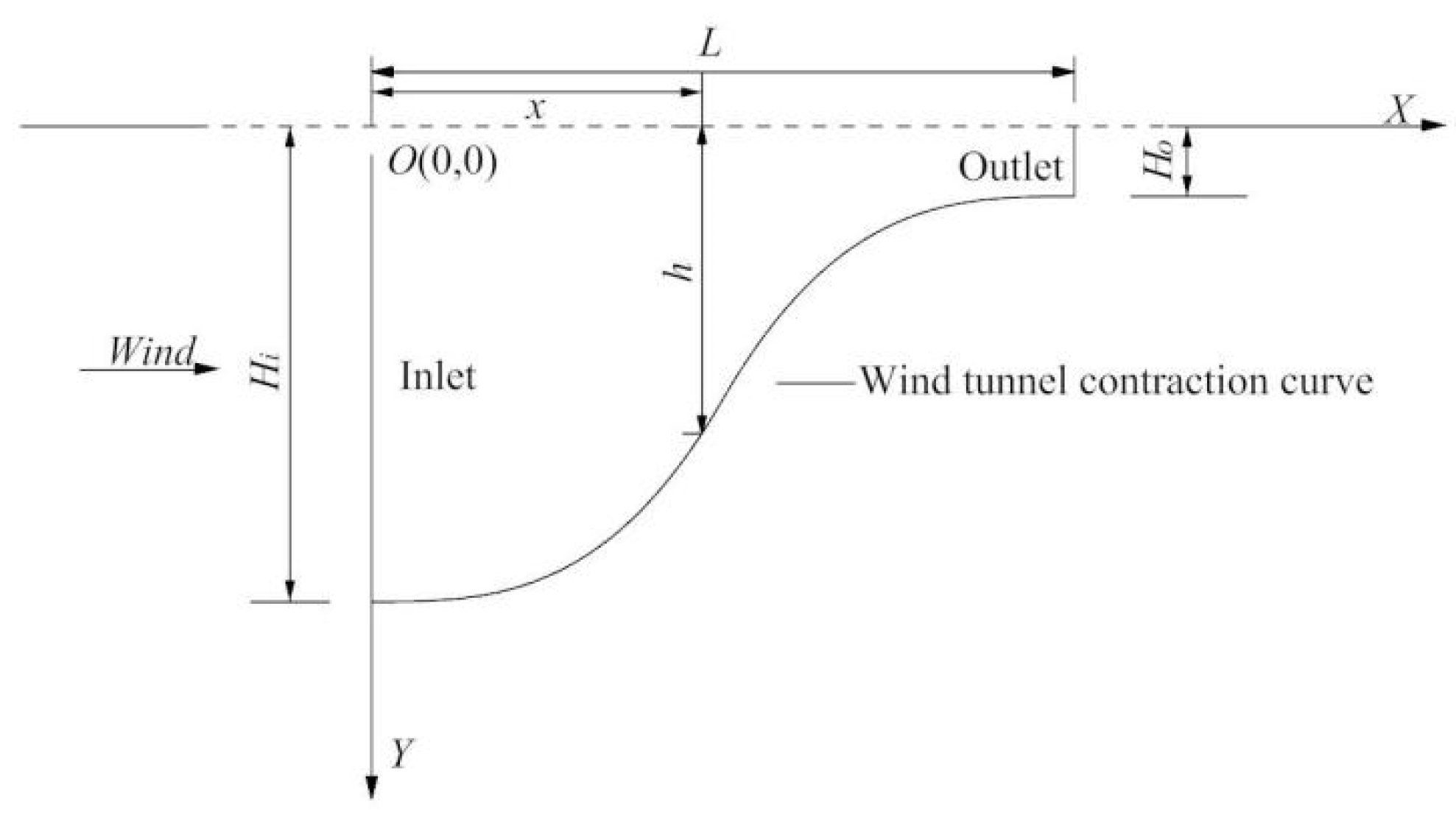
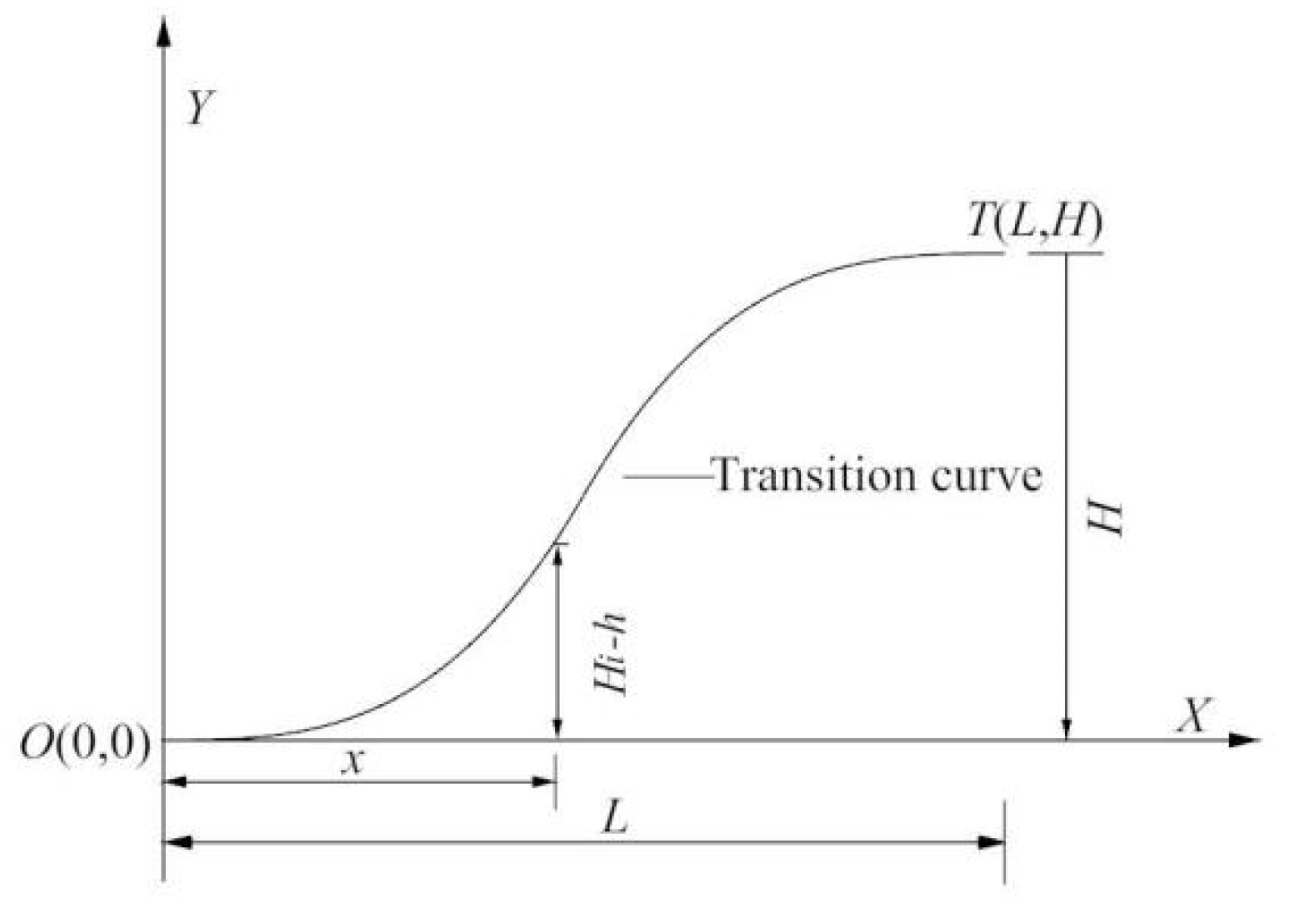
2. Wind Tunnel Contraction Transition Curve

The transition section of the terrain model can be studied with reference to the wind tunnel contraction curve [27,28]. The main considerations in the design of the wind tunnel contraction section are that the fluid does not separate at the contraction section outlet and that the outlet flow field is uniform, parallel, and stable. Wind tunnel contraction curves have been widely used as the terrain transition curve. At present, three types of wind tunnel contraction curves are commonly used, namely, bi-cubic, Witoszynski, and quantic.

The wind tunnel contraction curve is shown in Figure 2. H_i and H₀ denote the inlet and outlet radii of the wind tunnel contraction section, respectively; h is the height of the wind tunnel contraction curve; x is the horizontal distance from any point to the curve start position O; L is the length of the curve. The wind tunnel contraction curve is converted to a terrain transition curve with reference to Figure 3. H is the height of the transition curve (H = H_i − H₀), and the transition curve is expressed as:

$$y=H_i-h$$

(1)

The bi-cubic wind tunnel contraction curve can be expressed as in Formula (2):

$$h=\{\begin{array}{c}{H}_i-\left(H_i-H_0\right)\frac{{(x/L)}^3}{{\left(x_f/L\right)}^2}\hspace{1em}x\le x_f\\ H_0+\left(H_i-H_0\right)\frac{{\left(1-x/L\right)}^3}{{\left(1-x_f/L\right)}^2}\hspace{1em}x\le x_f\end{array}$$

(2)

where $x_f$ is the coordinate of the curve inflection point, generally set as 0.5. According to Equation (1), the bi-cubic transition curve (BCTC) can be expressed as follows:

$$y=\{\begin{array}{c}H\frac{{(x/L)}^3}{{\left(x_f/L\right)}^2}\hspace{1em}x\le x_f\\ H\left[1-\frac{{\left(1-x/L\right)}^3}{{\left(1-x_f/L\right)}^2}\right]\hspace{1em}x\le x_f\end{array}$$

(3)

Huang et al. [26] proposed an improved Witoszynski transition curve (WTC) for the terrain transition section by deriving the Witoszynski curve formula:

$$y=H\left\{1-\frac{{\left[1-{\left(x/L\right)}^2\right]}^2}{{\left[1+A{\left(x/L\right)}^2\right]}^3}\right\}$$

(4)

where A is a constant, generally set as 1/3.

The inlet smoothness of the quantic curve is higher than that of the Witoszynski curve and is not prone to separation. Moreover, the outlet is flatter and more continuous than the bi-cubic curve, with a more uniform velocity field. The quantic curve can be expressed as:

$$h=H_i\left\{\eta \left[1-\left(\frac{H_0}{H_i}\right)\right]+1\right\}$$

(5)

where $\eta =-10{\epsilon }^3+15{\epsilon }^4-6{\epsilon }^5$, $\epsilon =x/L$.

Brassard et al. [29] improved the quantic curve by optimizing the radius of curvature at the contraction section inlet and outlet. Thus, the inlet and outlet in this curve are smoother than those in the original quantic curve.

$$h=H_i{\left\{\eta \left[1-{\left(\frac{H_0}{H_i}\right)}^{1/f(\epsilon )}\right]+1\right\}}^{f(\epsilon )}$$

(6)

where f (ε) is a constant but can also be a function that varies with the value of b, set as 0.3, 0.5, 0.7, 1, 2, $x/L$, $(x/L{)}^2$, and $(x/L{)}^3$. Based on Equation (1), the quantic transition curve (QTC) can be expressed as follows:

$$y=H_i-H_i{\left\{\eta \left[1-{\left(\frac{H_0}{H_i}\right)}^{1/f(\epsilon )}\right]+1\right\}}^{f(\epsilon )}$$

(7)

Since the quantic curve has superior flow characteristics, this research is based on the improved quantic curve proposed by Brassard. The parameters of the curve are optimized and set with reference to the design principle of the wind tunnel contraction section. The optimized and improved quantic curve is used as the terrain transition curve. In general, to decrease turbulence, the contraction ratio should be large [30]. Usually, the wind tunnel contraction ratio ranges from 7 and 10, and in this study, the contraction ratio is set as 9, i.e., the area ratio of the inlet to the outlet is 9. According to Bell et al. [31], to ensure that the inlet and outlet boundary layers do not separate, the length L of the contraction section should range from 0.667H_i to 1.79H_i. Each parameter of the curve is set with reference to the common scale ratio of complex terrain models constructed at home and abroad. The scale ratio is 1:1500, and the parameters are set as H_i = 0.45 m and H₀ = 0.15 m. The maximum height of the transition curve connecting the terrain model edge is y = 0.3 m, and the equivalent slope is 1. The transition performance of each transition curve is compared under the same settings of the contraction ratio, length, and height. The transition curves of different terrains are shown in Figure 4.

3. Numerical Calculation

To compare the effects of various types of transition curves, we selected 10 cases in

Table 1. CI for different transition curves.

	f(ε) = 0.3	f(ε) = 0.5	f(ε) = 0.7	f(ε) = 1	f(ε) = 2	f(ε) = x/L	f(ε) = x2/L2	f(ε) = x3/L3	BCTC	WTC
Sx	0.07	0.11	0.07	0.07	0.02	0.03	0.09	0.20	0.03	0.02
Ax	0.68	0.66	0.68	0.72	0.80	0.79	0.65	1.04	0.81	0.82
Tx	4.25	5.10	3.59	3.55	3.52	3.61	4.67	6.03	3.52	3.53
CI	1.04	1.31	0.97	1.00	0.81	0.83	1.16	1.95	0.83	0.82

. It would be very time-consuming to perform 3D numerical simulations, so alternatively, 2D simulations were conducted in this section. Additionally, several previous studies also apply 2D number simulation to study the transition effect of transition curves [14,26,28]. Note that the 3D simulations were applied to verify the results in a real case in Section 4.

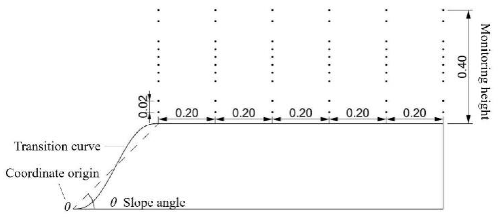
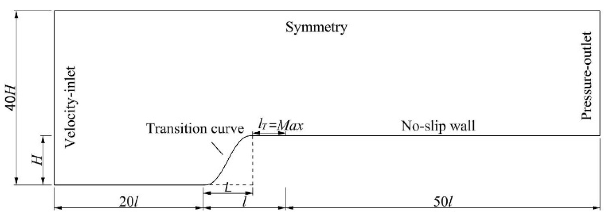
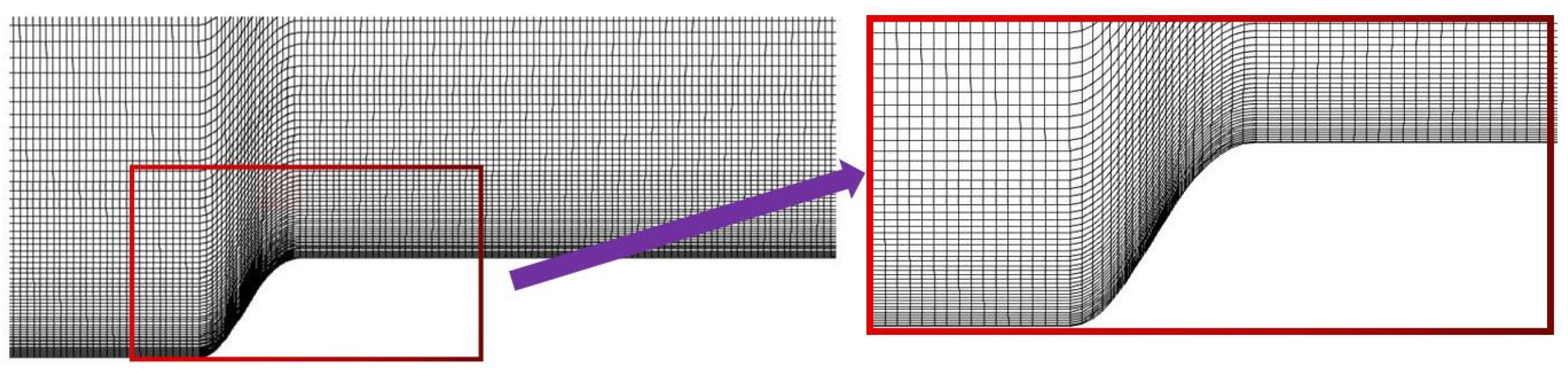
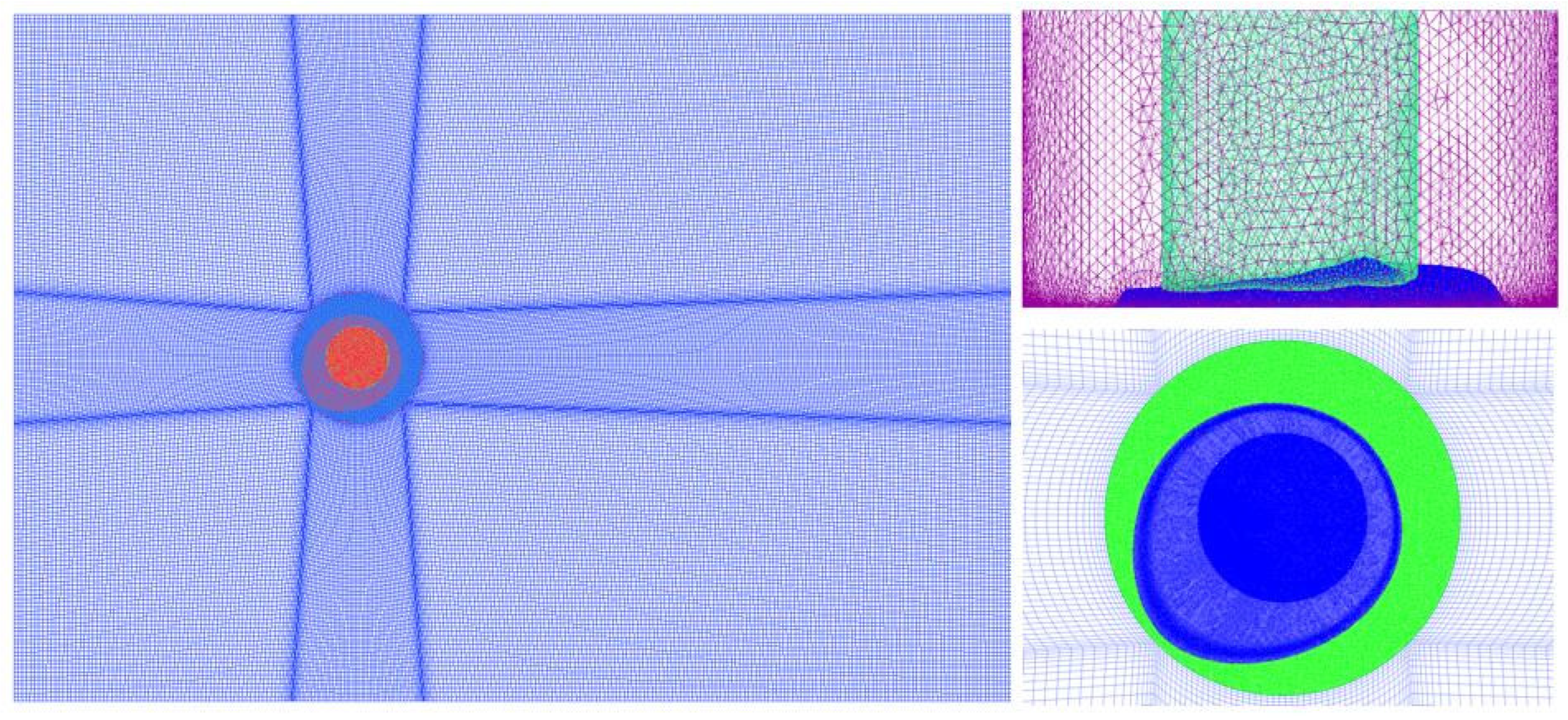
3.1. Parameter Setting and Meshing

To compare the flow characteristics of different transition curves, six monitoring positions are set on the horizontal line connected to the end of the curve, as shown in Figure 5. The horizontal spacing of each position is 0.20 m; the horizontal distance l_T from the end of the curve is 0, 0.2 m, 0.4 m, 0.6 m, 0.8 m, and 1 m; the height of each monitoring position is 0.4 m; the vertical distance between two adjacent monitoring points is 0.02 m. The computational domain and boundary conditions are set, as shown in Figure 6. The distance between the origin of the transition curve and the inlet boundary is 20l (l is the combined horizontal projection length of the transition curve), and the combined transition curve is 50l from the outlet boundary. The height of the computational domain is 40 m, and the blockage ratio is less than 3% [32]. The inlet boundary condition of the computational domain is defined as the velocity inlet boundary condition; the uniform turbulence intensity profile is set as 5%, which aligns with the study by Huang et al. [26]; the inlet wind speed profile adopts the exponential form, as shown in Equation (8); the top and sides of the computational domain are set as symmetric boundaries; the domain bottom is set as a non-slip wall, and the outlet condition is set as a pressure outlet.

$$U_x=U_r{\left(\frac{z}{z_r}\right)}^{\alpha }$$

(8)

where U_x is the wind speed at height z, U_r is the wind speed (3 m/s) at a reference height z_r = 10 m (scale height 0.007 m), the gradient wind height wind speed is 5.3 m/s, and α is set as 0.15.

The SST k–ω model is used as the turbulence model, the pressure and velocity coupling method pertain to the SIMPLEC algorithm, the momentum and turbulent kinetic energy dispersion method are set to have the second-order upwind format, the calculation residual is set as 10⁻⁶, and the transient solution with a time step of 0.001 s and 10,000 steps is adopted. Three mesh schemes (cases 1–3) are considered, with the number of meshes being 0.6 million, 0.9 million, and 1.6 million, respectively. The first grid height is set as 7 × 10⁻⁵ m and a growth factor of 1.05, which aligns with the study by Huang et al. [26]. The calculated y+ value is approximately 1, which satisfies the requirements of the turbulence model for solving the near boundary layer viscous region [33]. The calculation results show that the difference in the wind velocity for cases 1, 2, and 3 is extremely small. Thus, case 1 is used as the mesh scheme considering the computational cost. The mesh for the transition section is shown in Figure 7.

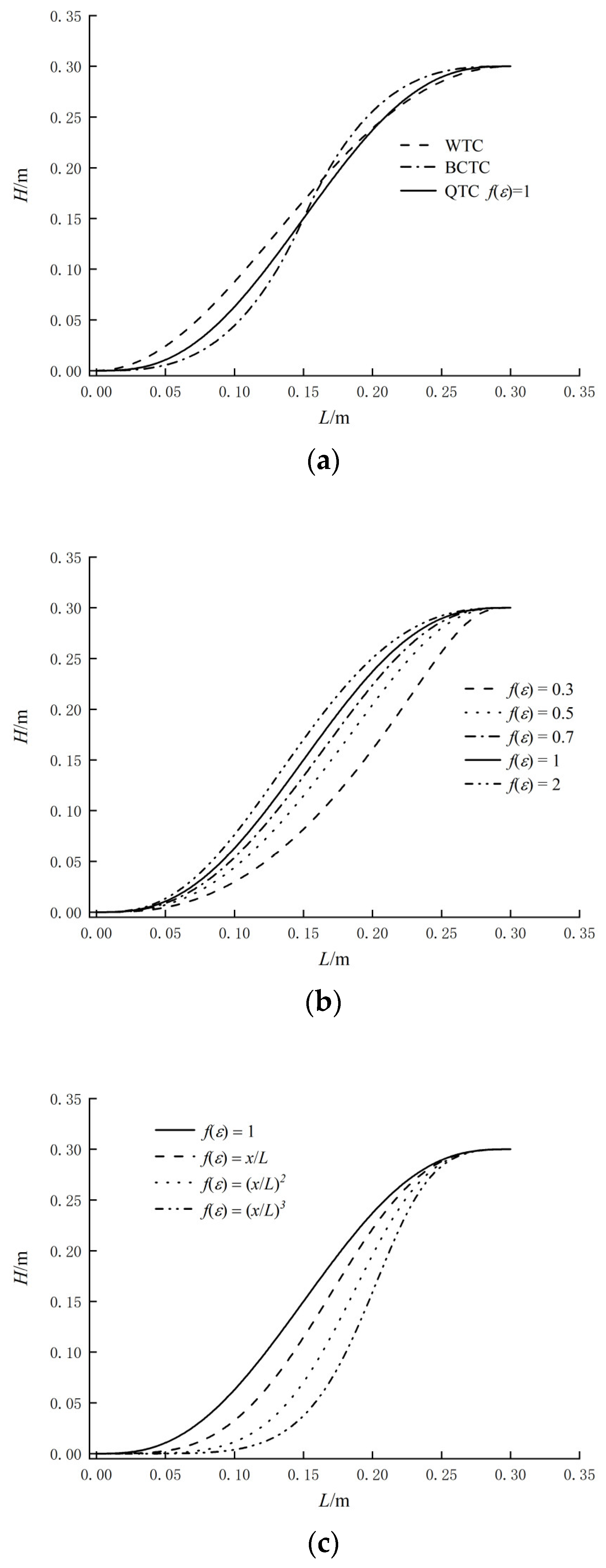
3.2. Transition Performance of Different Transition Curves

After the incoming wind passes through the transition section, the airflow is compressed by the transition section. The wind speed, attack wind angle, and turbulence intensity change to a certain extent with the inlet conditions. In particular, a smaller degree of change corresponds to a superior performance of the transition section. To evaluate the transition performance of the transition curve, we define the wind speed variation rate S_x, mean wind angle of attack A_x, and turbulence intensity variation rate T_x as follows:

$$S_x={\displaystyle {\sum }_{i=1}^N\frac{\left|V_i-V_{oi}\right|}{V_{oi}}}\cdot \frac{\Delta h_i}{H_w}$$

(9)

$$A_x={\displaystyle {\sum }_{i=1}^N\frac{\left|a_i\right|\cdot \Delta h_i}{H_w}}$$

(10)

$$T_x={\displaystyle {\sum }_{i=1}^N\frac{\left|T_i-T_{oi}\right|}{T_{oi}}}\cdot \frac{\Delta h_i}{H_w}$$

(11)

where N is the number of monitoring points, V_i is the mean wind speed at the i-th monitoring point from the wall, and V_oi is the mean wind speed at the i-th monitoring point from the wall at the inlet. Δh_i is the vertical distance between two adjacent monitoring points, a_i is the mean wind attack angle at the i-th monitoring point from the wall, T_i is the turbulence at the i-th monitoring point from the wall, and T_oi is the turbulence at the i-th monitoring point from the wall at the inlet.

The wind speed variation rate, mean wind attack angle, and turbulence variation rate of different transition curves are shown in Figure 8.

Figure 8 shows that the mean wind speed variation rate of different transition curves decreases. When f (ε) = 0.5 and f (ε) = $(x/L{)}^3$, S_x of the QTC curve increases and later decreases with increasing distance behind the transition curve, and S_x is larger at the x = 1.0 m position than that at the other curves. A_x of the QTC curve with parameter f(ε) = $(x/L{)}^3$ increases and later decreases. A_x is larger than the other curves, and the A_x of other transition curves decreases with increasing distance behind the transition curve. With the increase in the distance behind the transition curve, T_x of the QTC transition curve with f (ε) = 0.3 increases, and T_x of the QTC transition curve with f (ε) = 0.5, f (ε) = $(x/L{)}^2$, and f (ε) = (x/L)³ increases and later decreases. T_x of the other transition curves is relatively smooth.

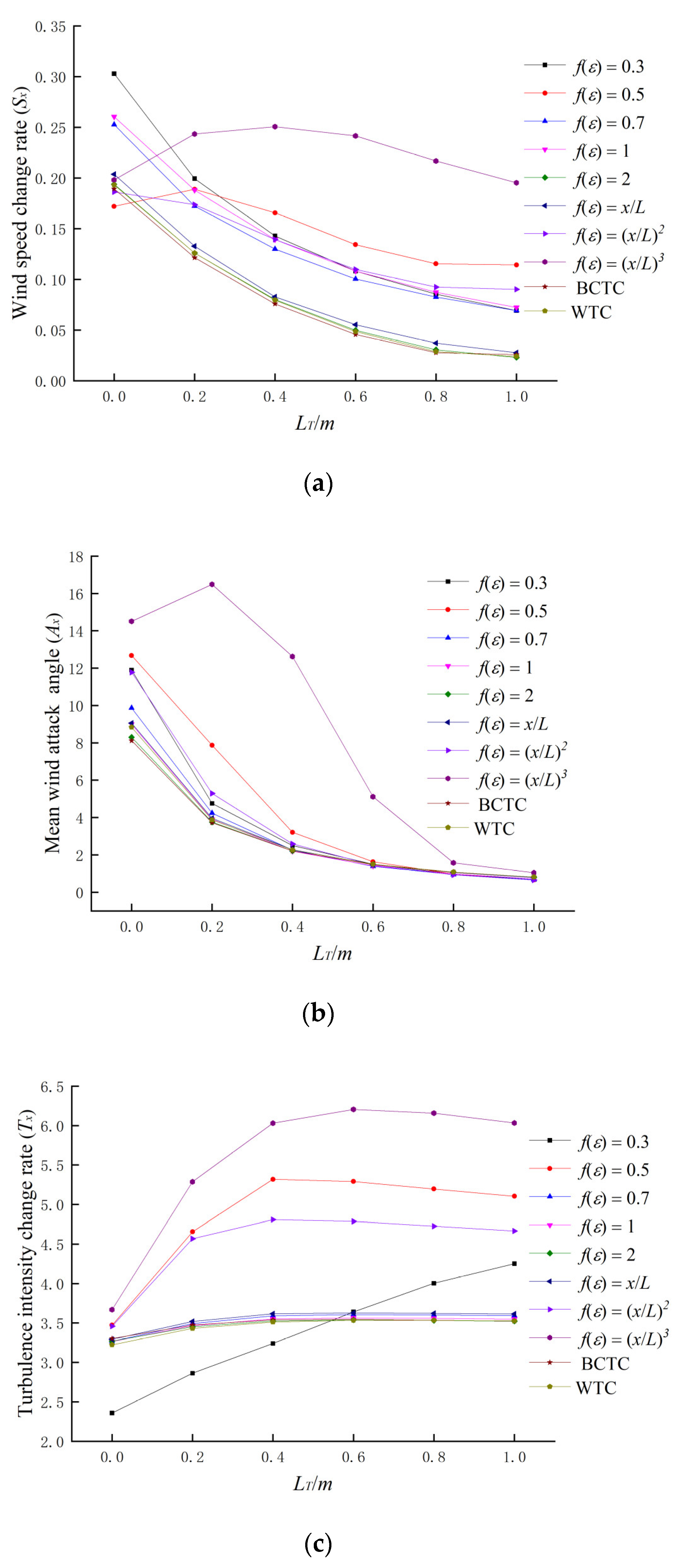
3.3. Evaluation of the Terrain Transition Curve

To evaluate the transition performance of transition curves with different parameters, the comprehensive evaluation index (CI) is proposed:

$$CI=\frac{1}{3}\left(\frac{S_x}{S_r}+\frac{A_x}{A_r}+\frac{T_x}{T_r}\right)$$

(12)

where S_x, A_x, and T_x denote the mean wind speed variation rate, mean wind attack angle, and turbulence intensity variation rate of the transition curve, respectively, and S_r, A_r, and T_r denote the corresponding values of the reference transition curve.

A smaller CI indicates a smaller difference between the incoming wind and the superior transition effect of the terrain transition curve. The CI values of each transition curve at x = 1 are presented in Table 1. The QTC transition curve with f (ε) = 2 has the smallest CI, which indicates that it has the smallest influence on the incoming wind and the highest transition performance.

3.4. Selection of Transition Curve

The design of the terrain transition section must satisfy two criteria: (1) The incoming wind must maintain the inlet reference wind characteristics as much as possible after passing through the terrain transition section. (2) The length of the transition from the beginning of the transition section to the time at which the airflow is stabilized should be as small as possible [34]. In summary, a larger terrain transition section increases the size of the computational domain and corresponds to the consumption of more computational resources. According to Figure 8, the QTC transition curve with f (ε) = 2 corresponds to the least changes in the wind speed variation rate, mean wind attack angle, and turbulence intensity variation rate with the end of the curve at x = 0.6 m after the curve. Therefore, the QTC (f (ε) = 2) wind tunnel contraction curve is selected as the terrain transition curve, and the length of the curve is x = 0.6 m after the curve. This curve is applied to the subsequent terrain modeling to examine the complex terrain wind environment.

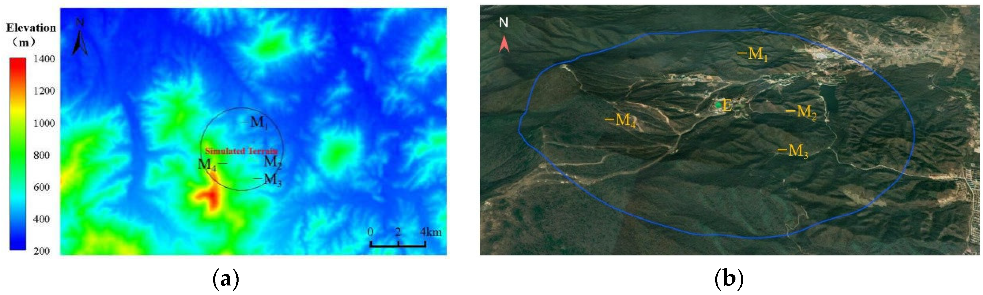
4. Yabuli Ski Resort Wind Field Simulation

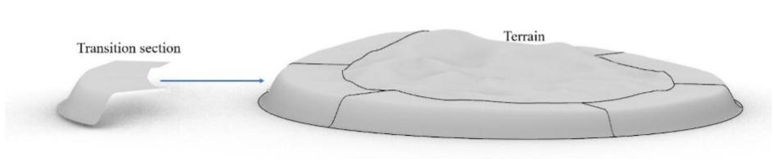
4.1. Terrain Model and Mesh

The Yabuli ski resort is located in a mountain forest area, and the ski resort and facility construction are typical and representative. The terrain is selected from the terrain image with ski resort monitoring point E (anemometer location) as the center and a radius of 3 km. Many high-altitude peaks are present around the ski resort. Mountains M₁–M₄, elevation, and corresponding images are shown in Figure 9. The wind environment is affected by the terrain of the adjacent mountains, the flow characteristics cannot be accurately classified, and the wind field environment in the ski resort area is highly complex.

The elevation data are obtained using the Advanced Spaceborne Thermal Emission and Reflection Radiometer Global Digital Elevation Model (ASTER GDEM) with a resolution of 30 m. The QTC transition curve with f (ε) = 2 is used to establish the terrain transition section to alleviate the influence of the ‘artificial cliff’. The terrain model is shown in Figure 10. To ensure that the incoming wind is fully developed from the inlet boundary to the complex terrain, the dimensions of the computational domain are set as 16D × 8D × H_d. D, the diameter of the simulated terrain, is 6 km, and the height of the computational domain H_d is 7 km. The distance from the inlet to the center of the terrain is 5.5D, the distance from the center of the terrain to the outlet is 10.5D, and the distance from the center of the terrain to both sides is 5.5D, which satisfies the requirement that the model blockage rate is less than 3%.

As shown in Figure 11, the computational domain is divided into three parts: the outer region, hollow cylindrical transition region, and inner cylindrical terrain region. To balance the computational accuracy and computational efficiency, a mixed tetrahedral and hexahedral mesh division method is used. The structured hexahedral mesh is chosen for the outer region due to concerns regarding the stages of the incoming flow and wake development. The transition region and terrain region, due to the irregular surface, adopt an unstructured tetrahedral mesh to discretize the region. Considering the complexity of the terrain, five prism layers are set at the terrain surface, with the first layer having a height of 2 m and a growth factor of 1.1. The total number of meshes is approximately 6.2 million.

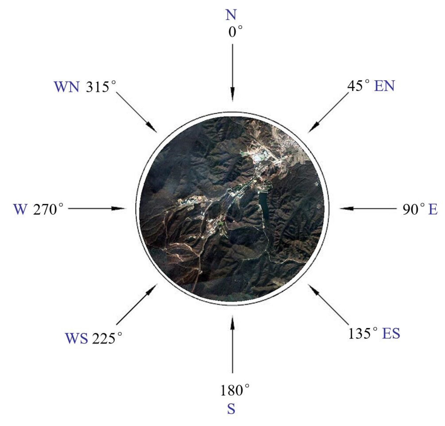
4.2. Parameter Setting and Calculation

Surface roughness is a key parameter for studying the vertical profile distribution of wind fields and influences the development of the near-surface boundary layer in the region. Thus, the roughness conditions are significant for the numerical simulation of wind fields [35]. To simulate the complex surface roughness, the wall function method is commonly used, and a Fluent framework is set by converting the roughness length z₀ to the roughness physical height k_s when incorporating the wall function. Blocken et al. [36] specified the relationship between the roughness length and roughness physical height, as expressed in (13).

$$k_s=\frac{9.793z_0}{C_s}$$

(13)

where C_s is the roughness constant, usually set as 0.5. According to the classification of the surface roughness by Wieringa [37], the surface roughness length z₀ in the terrain area is set as 0.03 m.

The top surface and two sides of the computational domain are set to have symmetric boundary conditions; the bottom surface, transition region, and terrain are set as no-slip boundary conditions; and the outlet has a pressure-out condition. The computational domain inlet is compiled using a user-defined function (UDF), and the velocity inlet follows Equation (8). The 10-m-height reference wind speed is set as 18 m/s according to the 30-y average daily maximum wind speed statistics at the nearby meteorological stations in the study area. The inlet conditions of the turbulent kinetic energy k and dissipation rate ω [26] are expressed in Equations (14) and (15), respectively.

$$k=\frac{3}{2}{\left(U_{x}I\right)}^2$$

(14)

$$\omega =\frac{k^{0.5}}{l{c}^{0.25}}$$

(15)

where the turbulence intensity I is set as 5%, the turbulence integration scale l is set as 500 m, and c is a constant set as 0.033.

The k–ω SST shear stress model is used as the turbulence model [38], and the pressure-based unsteady state solver and SIMPLEC algorithm are used for the coupled pressure-velocity treatment. The gradient interpolation method is Green–Gauss node based, and the discrete control format for the momentum, turbulent kinetic energy, and dissipation rate is second-order windward.

To study the impact of terrain on the ski resort area wind environment regarding different incoming wind directions, multiple wind directions are simulated by rotating the terrain and mesh of the transition area. The calculation case involves 8 incoming wind directions, as shown in Figure 12. We define 0° as the positive north wind direction. The clockwise rotation of the incoming wind direction is positive, with each 45° rotation corresponding to one case, and the incoming wind direction for cases 1 to 8 ranges from 0° to 315°.

4.3. Simulation Results and Analysis

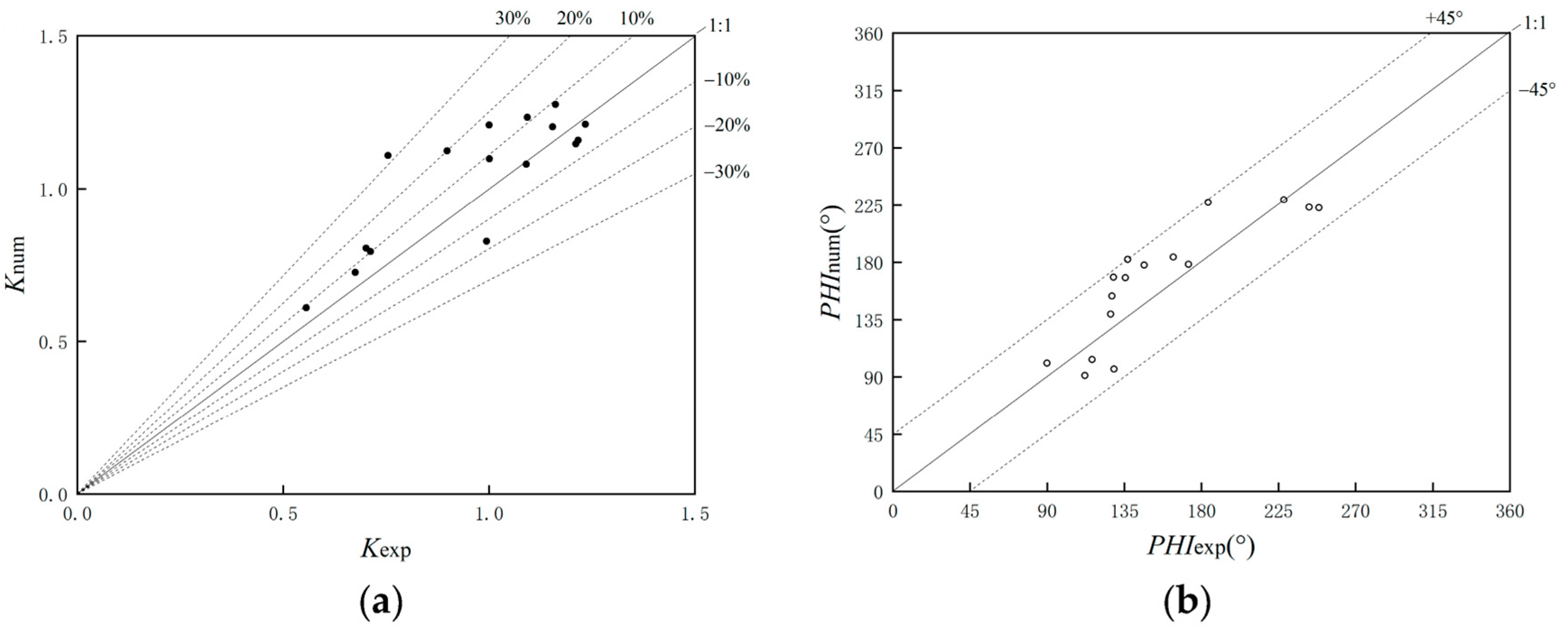
4.3.1. CFD Numerical Simulation Validation

Five anemometers are deployed near the ski racetrack to collect wind speed data. In particular, British GILL ultrasonic anemometers are used, with a wind speed measurement range of 0–65 m/s, accuracy of 0.01 m/s, wind direction resolution of 1°, and wind speed collection frequency of 4 Hz. The anemometer installation height is approximately 3 m from the ground, A–E are the deployment positions of the anemometer, and the site anemometer deployment location is shown in Figure 13. Two-month (December 2020 to January 2021) actual field measurement statistics of observation point E are shown in Figure 14. The 10-min average wind direction is mostly 90°–235°, and the probability of a mean wind speed of 2–5 m/s is 61.29%.

To compare the CFD numerical simulation results with the wind speed and wind direction measured in the field, we define the wind speed ratio K, the ratio of the wind speed at the observed position compared to that at the position of the reference point (observation point E). According to the statistical results of the mean wind direction measured in the field, the simulated wind speed ratio under four wind directions from 90° to 235° is compared and analyzed with the measured wind speed ratio, as shown in Figure 15a. The error between the simulated wind speed ratio (K_num) and measured wind speed ratio (K_exp) is within 20%, indicating that the simulated and measured wind speed ratios in the corresponding directions agree. Figure 15b shows the numerically simulated wind direction (PHI_num) corresponding to the field-measured direction (PHI_exp). The simulated wind direction is within the wind direction angle of 45° from the field measurement.

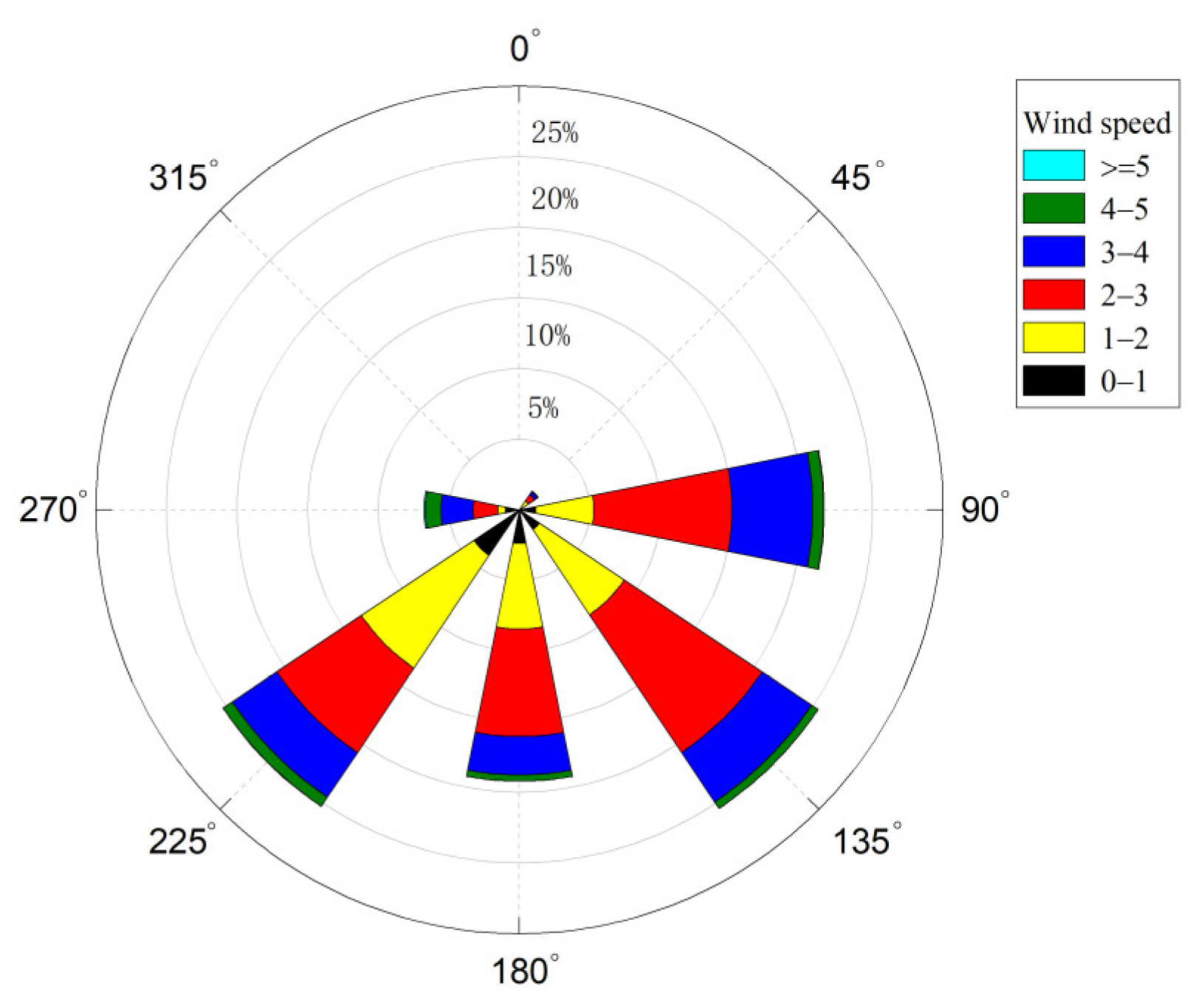
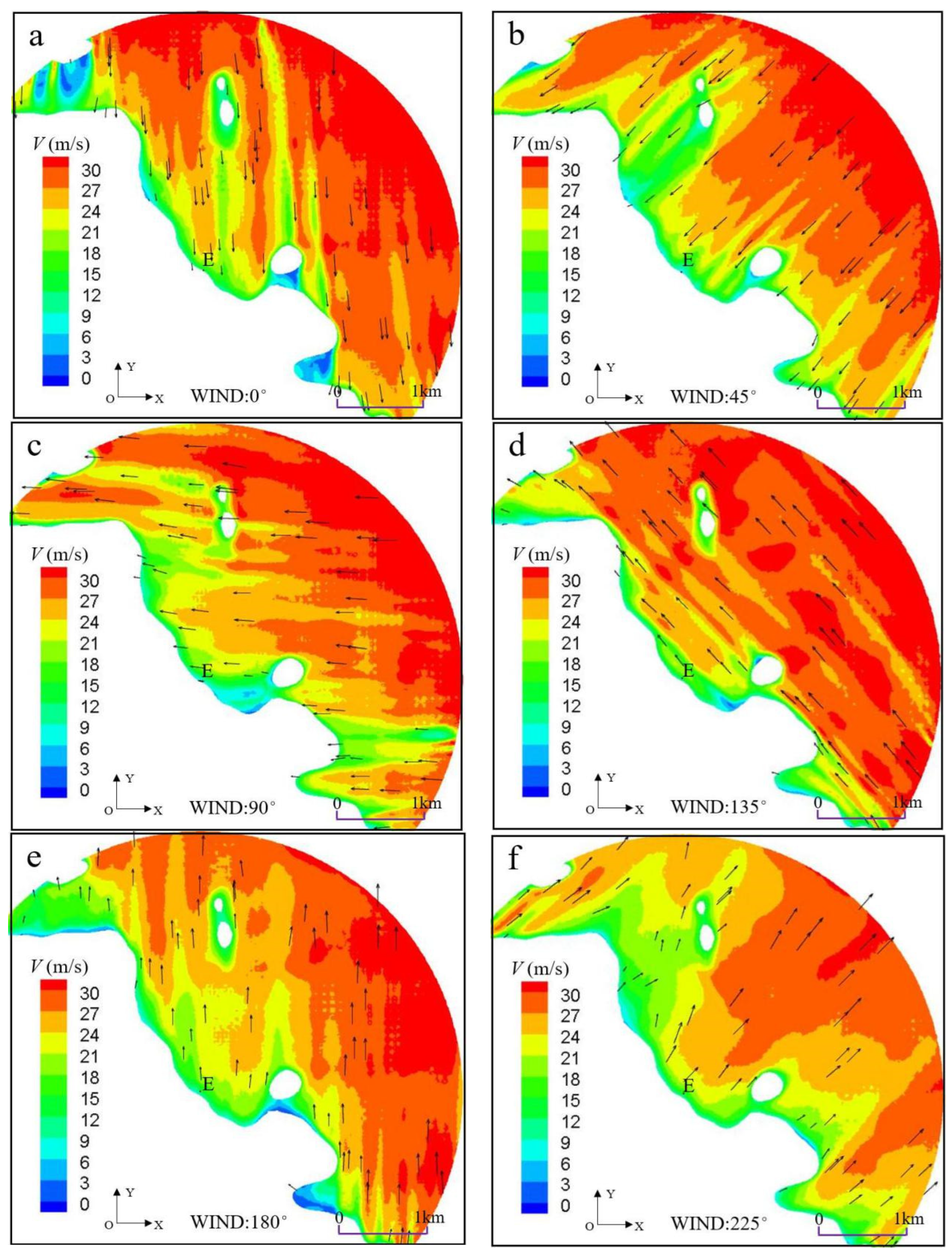
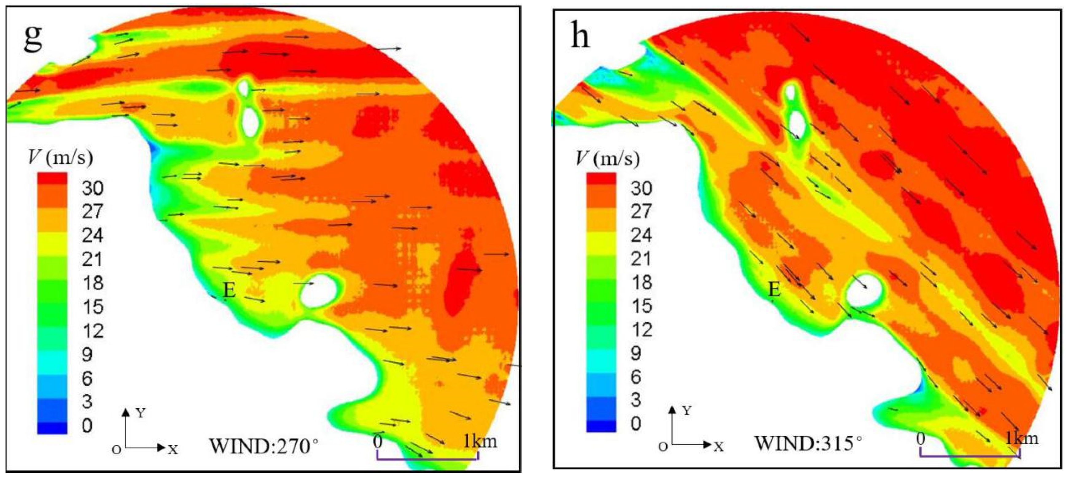
4.3.2. Ski Resort Area Wind Environment

The ski resort racetrack area lies in the concave section of the terrain, and the plane wind speed at the altitude of observation point E is considered to study the influence of the terrain on the ski resort area wind environment under different incoming wind directions. The wind speed cloud map of the ski resort area is shown in Figure 16. Subfigures a–h show the cloud map of 8 incoming directions (0°–315°), with each 45° corresponding to one case. The black arrow in the map indicates the wind direction, and the white part of the terrain range is the cross-section of the mountain at the altitude of observation point E.

When the incoming wind direction is 0°, the incoming wind flow appears to accelerate between mountains M₁ and M₄, and the wind speed gradually decreases until it reaches point E of the racetrack. When the incoming wind direction is 45°, mountains M₁ and M₂ block the incoming wind, and the wind speed decreases when the incoming wind reaches observation point E near the racetrack. When the incoming wind direction is 90°, the wind speed is reflected by mountain M₄, and the wind speed is relatively low when the incoming wind reaches observation point E. When the incoming wind direction is 135°, the wind speed decreases near observation point E and gradually increases towards the open area. When the incoming wind direction is 180°, the incoming wind is blocked by mountains M₃ and M₄, and the wind speed is low. When the incoming wind direction is between 225° and 270°, mountain M₄ blocks the incoming wind, and the wind speed near observation point E is low. When the wind direction is 315°, the terrain near mountain M₄ tends to block the incoming wind. The incoming wind does not undergo the canyon acceleration effect between mountains M₁ and M₄, and the wind speed gradually increases until the wind reaches observation point E. The direction of the wind flow is influenced by the neighboring mountains, with the effect being more notable at 225° and 270° in the direction of the incoming wind. The numerical results are consistent with the conventional distribution characteristics of the topographic wind field in this study area, which further verifies the accuracy of the numerical simulation of this study. Overall, the wind environment in the ski resort area is significant when the incoming wind direction is between 0° and 315°. In the case of high wind speeds, the wind resistance design of buildings and ancillary facilities in the ski resort area must be considered.

In this Section, the application case of the transition curve, which is used to verify the feasibility of the transition curve, mainly focuses on the mean wind profile on complex terrain. The comprehensive analysis of the wind environment regarding turbulence intensity, turbulence integral length scale, fluctuating wind spectra, and gust factor will be studied in the future.

5. Conclusions

Considering the influence of the wind tunnel contraction section outlet on the uniformity and stability of the airflow, a terrain transition curve is derived based on the wind tunnel contraction curve. Different transition curves are analyzed and evaluated through 2D numerical simulations, and a terrain model boundary transition curve suitable for mountainous wind fields is proposed. The proposed transition curves are applied to model the terrain of complex mountain ski resort areas, and CFD numerical simulations are performed to verify the accuracy of the numerical simulations in comparison with the field measurement results. The following conclusions are derived:

• The transition curve proposed in this paper has the best performance compared with the existing transition curves. The mean wind speed variation rate, mean wind attack angle, and turbulence intensity variation rate of the QTC transition curve with f (ε) = 2 are relatively small. The comprehensive evaluation index value (CI) is smaller than that of the other transition curves, which indicates that the impact on the wind characteristics of the incoming wind is the smallest, and the transition performance is the highest.
• The proposed terrain transition curve has good applicability in mountainous terrain modeling. The proposed terrain transition curve is applied to complex mountainous terrain modeling and CFD numerical simulations. Comparison of the wind speed ratio associated with numerical simulations and field measurements, and the error is basically within 20%, indicating a reasonable agreement.
• The terrain transition section is applied to model complex mountainous areas, which can make the incoming wind smoothly transition to the terrain area and reduce the impact of “artificial cliffs” on the numerical simulation results. This method can be applied to CFD numerical simulations to effectively reflect the wind environment characteristics of the ski resort area, which has good applicability to practical engineering and provide a reference for the wind resistance design with complex terrain.

References

- Huang, G.; Jiang, Y.; Peng, L.; Solari, G.; Liao, H.; Li, M. Characteristics of intense winds in mountain area based on field measurement: Focusing on thunderstorm winds. J. Wind Eng. Ind. Aerodyn. 2019, 190, 166–182. [Google Scholar] [CrossRef]
- Jing, H.; Liao, H.; Ma, C.; Tao, Q.; Jiang, J. Field measurement study of wind characteristics at different measuring positions in a mountainous valley. Exp. Therm. Fluid Sci. 2020, 112, 109991. [Google Scholar] [CrossRef]
- Song, J.L.; Li, J.W.; Flay, R.G.J. Field measurements and wind tunnel investigation of wind characteristics at a bridge site in a Y-shaped valley. J. Wind Eng. Ind. Aerodyn. 2020, 202, 104199. [Google Scholar] [CrossRef]
- Ren, W.; Pei, C.; Ma, C.; Li, Z.; Wang, Q.; Chen, F. Field measurement study of wind characteristics at different measuring positions along a bridge in a mountain valley. J. Wind Eng. Ind. Aerodyn. 2021, 216, 104705. [Google Scholar] [CrossRef]
- Jiang, F.; Zhang, M.; Li, Y.; Zhang, J.; Qin, J.; Wu, L. Field measurement study of wind characteristics in mountain terrain: Focusing on sudden intense winds. J. Wind Eng. Ind. Aerodyn. 2021, 218, 104781. [Google Scholar] [CrossRef]
- Hui, M.C.H.; Larsen, A.; Xiang, H.F. Wind turbulence characteristics study at the Stonecutters Bridge site: Part I-Mean wind and turbulence intensities. J. Wind Eng. Ind. Aerodyn. 2009, 97, 22–36. [Google Scholar] [CrossRef]
- Huang, G.; Peng, L.; Liao, H.; Li, M. Field measurement study on wind characteristics at Puli great bridge site in mountainous area. Xinan Jiaotong Daxue Xuebao/J. Southwest Jiaotong Univ. 2016, 51, 349–356. [Google Scholar] [CrossRef]
- Tamura, Y.; Suda, K.; Sasaki, A.; Iwatani, Y.; Fujii, K.; Ishibashi, R.; Hibi, K. Simultaneous measurements of wind speed profiles at two sites using Doppler sodars. J. Wind Eng. Ind. Aerodyn. 2001, 89, 325–335. [Google Scholar] [CrossRef]
- Mattuella, J.M.L.; Loredo-Souza, A.M.; Oliveira, M.G.K.; Petry, A.P. Wind tunnel experimental analysis of a complex terrain micrositing. Renew. Sustain. Energy Rev. 2016, 54, 110–119. [Google Scholar] [CrossRef]
- Hu, P.; Li, Y.; Xu, G.J.; Han, Y.; Cai, C.S.; Xue, F. Investigation of the longitudinal wind power spectra at the gorge terrain. Adv. Struct. Eng. 2017, 20, 1768–1783. [Google Scholar] [CrossRef]
- Lystad, T.M.; Fenerci, A.; Øiseth, O. Evaluation of mast measurements and wind tunnel terrain models to describe spatially variable wind field characteristics for long-span bridge design. J. Wind Eng. Ind. Aerodyn. 2018, 179, 558–573. [Google Scholar] [CrossRef]
- Zhang, M.; Zhang, J.; Li, Y.; Yu, J.; Zhang, J.; Wu, L. Wind characteristics in the high-altitude difference at bridge site by wind tunnel tests. Wind Struct. An Int. J. 2020, 30, 547–558. [Google Scholar] [CrossRef]
- Chen, F.; Peng, H.; Chan, P.W.; Zeng, X. Wind tunnel testing of the effect of terrain on the wind characteristics of airport glide paths. J. Wind Eng. Ind. Aerodyn. 2020, 203, 104253. [Google Scholar] [CrossRef]
- Hu, P.; Li, Y.; Huang, G.; Kang, R.; Liao, H. The appropriate shape of the boundary transition section for a mountain-gorge terrain model in a wind tunnel test. Wind Struct. An Int. J. 2015, 20, 15–36. [Google Scholar] [CrossRef]
- Li, Y.L.; Xu, X.Y.; Zhang, M.J.; Xu, Y.L. Wind tunnel test and numerical simulation of wind characteristics at a bridge site in mountainous terrain. Adv. Struct. Eng. 2017, 20, 1223–1231. [Google Scholar] [CrossRef]
- Zhang, Y.; Tang, J.W.; Zhou, M.; Gao, L. Experimental research on the spatial distribution characteristics of wind field in valley terrain. Zhendong yu Chongji/J. Vib. Shock 2016, 35, 35–40. [Google Scholar] [CrossRef]
- Yamaguchi, A.; Ishihara, T.; Fujino, Y. Experimental study of the wind flow in a coastal region of Japan. J. Wind Eng. Ind. Aerodyn. 2003, 91, 247–264. [Google Scholar] [CrossRef]
- Yan, B.W.; Li, Q.S. Coupled on-site measurement/CFD based approach for high-resolution wind resource assessment over complex terrains. Energy Convers. Manag. 2016, 117, 351–366. [Google Scholar] [CrossRef]
- Tang, X.Y.; Zhao, S.; Fan, B.; Peinke, J.; Stoevesandt, B. Micro-scale wind resource assessment in complex terrain based on CFD coupled measurement from multiple masts. Appl. Energy 2019, 238, 806–815. [Google Scholar] [CrossRef]
- Uchida, T.; Sugitani, K. Numerical and Experimental Study of Topographic Speed-Up Effects in Complex Terrain. ENERGIES 2020, 13, 3896. [Google Scholar] [CrossRef]
- Tang, H.; Li, Y.; Shum, K.M.; Xu, X.; Tao, Q. Non-uniform wind characteristics in mountainous areas and effects on flutter performance of a long-span suspension bridge. J. Wind Eng. Ind. Aerodyn. 2020, 201, 104177. [Google Scholar] [CrossRef]
- Cheynet, E.; Liu, S.; Ong, M.C.; Bogunović Jakobsen, J.; Snæbjörnsson, J.; Gatin, I. The influence of terrain on the mean wind flow characteristics in a fjord. J. Wind Eng. Ind. Aerodyn. 2020, 205, 104331. [Google Scholar] [CrossRef]
- Blocken, B.; van der Hout, A.; Dekker, J.; Weiler, O. CFD simulation of wind flow over natural complex terrain: Case study with validation by field measurements for Ria de Ferrol, Galicia, Spain. J. Wind Eng. Ind. Aerodyn. 2015, 147, 43–57. [Google Scholar] [CrossRef]
- Ren, H.; Laima, S.; Chen, W.-L.; Zhang, B.; Guo, A.; Li, H. Numerical simulation and prediction of spatial wind field under complex terrain. J. Wind Eng. Ind. Aerodyn. 2018, 180, 49–65. [Google Scholar] [CrossRef]
- Ha, T.; Lee, I.; Kwon, K.; Lee, S.-J. Development of a micro-scale CFD model to predict wind environment on mountainous terrain. Comput. Electron. Agric. 2018, 149, 110–120. [Google Scholar] [CrossRef]
- Huang, G.; Cheng, X.; Peng, L.; Li, M. Aerodynamic shape of transition curve for truncated mountainous terrain model in wind field simulation. J. Wind Eng. Ind. Aerodyn. 2018, 178, 80–90. [Google Scholar] [CrossRef]
- Wolf, T. Design of a variable contraction for a full-scale automotive wind tunnel. J. Wind Eng. Ind. Aerodyn. 1995, 56, 1–21. [Google Scholar] [CrossRef]
- Liu, Z.-W.; Chen, X.-Y.; Chen, Z.-Q. Optimization of Transition Sections Around Terrain Model at Mountain Canyon Bridge Site. China J. Highw. Transp. 2019, 32, 266–278. [Google Scholar]
- Brassard, D.; Ferchichi, M. Transformation of a polynomial for a contraction wall profile. J. FLUIDS Eng. ASME 2005, 127, 183–185. [Google Scholar] [CrossRef]
- Zhou, G.; Wang, J.D.; Chen, H.S.; Chen, D.R. Optimized design of the contraction in a minitype high-speed water-tunnel. Chuan Bo Li Xue/J. Sh. Mech. 2009, 13, 513–521. [Google Scholar] [CrossRef]
- Bell, J.H.; Mehta, R.D. Contraction design for small low-speed wind tunnels. Nasa Sti/Recon Tech. Rep. N 1988, Contract NAS2-NCC-2-294. [Google Scholar]
- Bekele, S.A.; Hangan, H. A comparative investigation of the TTU pressure envelope -Numerical versus laboratory and full scale results. Wind Struct. An Int. J. 2002, 5, 337–346. [Google Scholar] [CrossRef]
- Hongmiao, J.; Haili, L.; Cunming, M.; Zhiguo, L. A study on boundary transition of a terrain model for wind field characteristics measurement. J. Vib. Shock 2020, 39, 178–207. [Google Scholar]
- Peng, H.; Yongle, L.; Haili, L. Shape of boundary transition section for mountains-gorge bridge site terrain model. Acta Aerodyn. Sin. 2013, 31, 231–238. [Google Scholar]
- Pattanapol, W.; Wakes, S.J.; Hilton, M.J.; Dickinson, K.J.M. Modeling of surface roughness for flow over a complex vegetated surface. Int. J. Eng. Nat. Sci. 2008, 2, 18–26. [Google Scholar]
- Blocken, B.; Stathopoulos, T.; Carmeliet, J. CFD simulation of the atmospheric boundary layer: Wall function problems. Atmos. Environ. 2007, 41, 238–252. [Google Scholar] [CrossRef]
- Wieringa, J. Updating the Davenport roughness classification. J. Wind Eng. Ind. Aerodyn. 1992, 41, 357–368. [Google Scholar] [CrossRef]
- Huang, W.; Zhang, X. Wind field simulation over complex terrain under different inflow wind directions. Wind Struct. 2019, 28, 239–253. [Google Scholar] [CrossRef]