Improved Gravity Wave Drag to Enhance Precipitation Simulation: A Case Study of Typhoon In-Fa

Abstract

Traditional gravity wave drag parameterizations produce wind stresses that are insensitive to changing horizontal resolution in numerical weather prediction (NWP), partly due to the idealized elliptical assumption. This study employs the modified subgrid-scale orography scheme based on the Fourier transform into gravity wave drag scheme of the China Meteorological Administration Global Forecast System (CMA-GFS) to assess its impacts on simulating precipitation during the slow-moving period of Typhoon In-Fa after its landfall in Zhejiang Province, China. The simulation with the updated scheme can effectively reduce the accumulated precipitation bias of the control one and improve the simulation of precipitation distribution and intensity, especially in the hourly precipitation simulation. The improved scheme primarily influences the wind field of the low-level troposphere and also changes the convergence of the integrated water vapor transport and ascending motions related to the reduced precipitation biases. The modified scheme enhances the tendencies of the horizontal winds caused by the varying horizontal resolutions in the model, strengthening the sensitivity of the gravity wave drag across the horizontal scales. Results from medium-range forecasts indicate the modified scheme benefits the statistics scores of precipitation over China and also reduces root-mean-square errors of 2 m temperature and 10 m winds.

1. Introduction

The interaction between the gravity wave drag (GWD) and atmospheric flows plays a critical role in the modulation of weather patterns [1]. Therefore, the gravity wave drag parameterization scheme emerges as one of the sources of simulation uncertainty in Numerical Weather Prediction (NWP) and Global Climate Model (GCM) simulations [2,3,4]. The study of Elvidge et al. [5] pointed out that the different smoothing and filtering methods treatments of the subgrid-scale orography (SSO) lead to variations in the standard deviation and the mean gradient of the SSO, resulting in the differences of wind stress simulation and hence global wind biases, causing systematic errors. Niekerk et al. [6] analyzed the current 11 operational numerical weather forecast models, including the typical climate model resolutions of around 100 km and seasonal forecast resolutions of around 40 km, and used kilometer-scale resolved model simulations as a reference. They indicated the total drag effects could yield up to 50% bias in simulations across the Northern and Southern Hemisphere. Additionally, studies [6,7,8] employing high resolution (kilometer-scale) carried out a diagnosis of the respective impacts of the resolved and the subgrid-scale parameterized parts in special regions of the Himalayas, Middle East, and the Rockies and evaluated the systematic biases in coarse-resolution models.

Despite years of development [9,10,11,12], current orographic drag parameterizations display deficiencies related to a lack of proper resolution sensitivity. Vosper et al. [7] discovered that the parameterized orographic gravity wave momentum fluxes are invariant with model horizontal resolution, resulting in a consistent underestimating of total gravity wave drag at coarser grid resolutions. These issues highlighted the need for developing a scheme that represents the subgrid-scale orographic drag across all the scales. Conventional schemes consider an idealized elliptical assumption, which is more suitable for isolated-type mountains, with a failure to fully capture the spectrum characteristics of subgrid-scale orography. When the horizontal resolution of models alters, it can easily lead to inaccurate wind stress from the gravity wave drag scheme, introducing systematic biases. Niekerk and Vosper [13] proposed a scale-aware gravity wave parameterization scheme across horizontal resolutions by directly applying the Fourier transform coefficients derived from the high-resolution model, which can help to reduce the excessive upper tropospheric horizontal wind speeds bias over both hemispheres in models at 130 km and 40 km resolutions.

Several studies explored the impacts of gravity wave drag schemes on simulating the atmospheric flow and precipitation characteristics over the monsoonal region of Eastern Asia [14,15,16,17]. Feng and Zhang [14] studied the thermal effects of the gravity wave drag, which can influence the simulations of vertical velocity and the moisture fields. They produced a more reasonable simulation of the heavy precipitation events during the Meiyu period in the Yangtze River. The studies by Zhong and Chen [16] and Choi and Hong [15] demonstrated that the adoption of the Flow-Blocking Drag (FBD) parameterization in the gravity wave drag scheme has essential impacts on the low-level tropospheric circulation and precipitation over East Asia. Zhang et al. [17] indicate that the FBD effect, along with the low-level gravity wave drag, plays a more critical role in weakening the anomalous summer monsoon circulation and excessive precipitation over land. Typhoon-induced precipitation is one of the common types of heavy precipitation in East Asia [18] and also one of the challenges for numerical models to simulate precipitation. The gravity wave drag scheme affects the extremely strong low-level winds of typhoons in the troposphere. This study mainly focuses on investigating the effects of the continuous hilly mountainous region in Zhejiang Province, China, on generating heavy precipitation for Typhoon In-Fa. Section 2 mainly introduces the major characteristics of Typhoon In-Fa and describes the numerical models and the modified parameterization scheme used in the study. Section 3 presents the main results, and Section 4 provides the summary and discussion.

2. Model and Method

2.1. Description of Typhoon In-Fa (2021)

Typhoon In-Fa (the sixth typhoon in 2021, After In-Fa) formed over the northwestern Pacific Ocean at 02:00 Beijing Time (BT) on 18 July [19,20,21,22]. On the morning of 19 July, it developed into a severe tropical storm, and then on 20 July, it turned into a typhoon. In-Fa intensified into a severe typhoon early on 21 July and traveled westward. At 1430 BT on 25 July, it made landfall on Zhoushan Island in Zhejiang Province with a maximum wind speed (MWS) of 38 m s⁻¹. On 26 July, In-Fa made another landing in Pinghu City, Zhejiang Province, after slowly traversing Hangzhou Bay. The average accumulated precipitation over Zhejiang Province was 191 mm [23] as a result of the slow movement in Hangzhou Bay for 16 h, breaking the record for total typhoon landfall precipitation in Zhejiang. The early stages of In-Fa supplied a tremendous amount of moisture to central China, contributing to the 21.7 heavy rainfall event in Henan Province [24,25].

The slow movement of In-Fa at Hang Zhou Bay is one of the reasons for the broken record of accumulated precipitation in Zhejiang Province, and the synoptic wind pattern is a critical component that produces the slow movement; therefore, the forecast wind became highly essential in the numerical forecast. The complex terrain of Zhejiang Province is oriented from northeast to southwest direction. The mountains are concentrated in the central to southern of the province, with peak elevations of about 2000 m. The intensity and spatial distribution of the precipitation over the area are significantly influenced by complicated orography distribution [26,27,28], and gravity wave drag is one of the essential terrain-induced physical processes. Therefore, it is meaningful to study the atmospheric wind pattern influenced by the terrain-induced gravity waves, particularly for the numerical simulation of the wind field of the low level of the troposphere.

2.2. The Method of “Scale-Aware” Orography Wave Drag Parameterization

The representation of the gravity wave drag schemes across horizontal scales introduces numerical simulation uncertainty [6], particularly in the selection of the high-resolution terrain dataset, smoothing method, and filter design, all of which can have a significant impact on the numerically simulated wind stresses at low-level troposphere and stratosphere [5]. According to Niekerk and Vosper [13], most models tend to underestimate the total surface drag terms, which include the resolved and parameterized components caused by orography.

Current gravity wave drag parameterizations in numerical weather forecasting and climate simulations often adopt an idealized elliptical for gravity wave drag parameterizations. Consequently, most models applying the assumption may inadequately represent the subgrid-scale orography and may not accurately represent the desired performance when the model grid sizes are varied [13]. Niekerk and Vosper [13] addressed a new method that employs the Fourier transforms to prevent the need for assumptions about the shape and distribution of the subgrid-scale topography and, as a result, to overcome the limitation of elliptical mountains.

The linear hydrostatic terms for the gravity wave momentum flux (${\tau }_{x,y})$ at the surface are written as

$${\tau }_{x,y}=A^{-1}\rho N{\int }_{-\mathrm{\infty }}^{\mathrm{\infty }}{\int }_{-\mathrm{\infty }}^{\mathrm{\infty }}\frac{\left(k,l\right)}{{\left(k^2+l^2\right)}^{1/2}}\left(Uk+Vl\right){\left|\widehat{h}\right|}^{2}dkdl,$$

(1)

where $\widehat{h}$ denotes the Fourier component, $\rho$ is the density, A is the area, and $k$ and $l$ l are the horizontal (zonal and meridional direction, respectively) wavenumbers in the grid size. The Brunt-Vaisala frequency N is represented as

$$\mathrm{N}=\sqrt{\frac{g}{\theta }\frac{d\theta }{dz}}.$$

(2)

The operational gravity wave drag scheme utilizes an idealized elliptical mountain with an assumption to describe the wave stress derived by Phillips (1984) from Equation (1). The surface terrain assumption in Equation (1) is expressed as

$$\mathrm{h}\left(x^{\prime },y^{\prime }\right)=h_0{\left[1+{\left(\frac{x^{\prime }}{a}\right)}^2+{\left(\frac{y^{\prime }}{b}\right)}^2\right]}^{-1}.$$

(3)

To implement Equation (1), it can be simplified to

$${\tau }_{x,y}=A^{-1}G\rho N{h}_0^{2}U.$$

(4)

Traditionally, the horizontal length scale of ellipses, denoted as $\left(a\right),$ can be replaced using the function of the standard deviation of subgrid topography $\left(\sigma \right)$, and the mean orographic slope aligned with the primary axis of the ellipse. The subgrid mountain height is given by

$$h_0=n\sigma ,$$

(5)

where $n=2.5$ is a tunable parameter.

Equation (1) can be represented as

$${\tau }_x,{\tau }_y=\mathsf{\rho }\mathrm{N}(\mathrm{U}{F}_1+V{F}_2,\mathrm{U}{F}_2+V{F}_3),$$

(6)

where

$$F_1=A^{-1}4{\pi }^2{\int }_{-\infty }^{\infty }{\int }_{-\infty }^{\infty }\frac{k^2}{K}{\left|\widehat{h}\right|}^{2}dkdl,$$

(7)

$$F_2=A^{-1}4{\pi }^2{\int }_{-\infty }^{\infty }{\int }_{-\infty }^{\infty }\frac{kl}{K}{\left|\widehat{h}\right|}^{2}dkdl,$$

(8)

$$F_3=A^{-1}4{\pi }^2{\int }_{-\infty }^{\infty }{\int }_{-\infty }^{\infty }\frac{l^2}{K}{\left|\widehat{h}\right|}^{2}dkdl,$$

(9)

$F_1, F_2$, and $F_3$ can directly employ the Fast Fourier transform or spherical harmonic transformation to extract coefficients at the corresponding resolution from high-resolution models.

2.3. CMA_GFS Model

This study applies the CMA_GFS global atmospheric model, containing fully compressible, non-hydrostatic equations that represent the entire atmosphere. A two-dimensional atmospheric reference state is used. It adopts a semi-Lagrangian and semi-implicit time integration scheme [29]. The terrain following the Charney-Phillips vertical variation configuration is utilized for the vertical coordinates, and the Arakawa-C horizontally staggered grid is used for spatial discretization [30]. The top of the CMA_GFS model is set at approximately 0.1 hPa and contains 87 levels with vertical and horizontal resolutions of 25 km. The long-wave and short-wave radiation schemes of the rapid radiative transfer model for general circulation models (RRTMG) [31], the modified NSAS cumulus parameterization [32,33], medium-range forecast planetary boundary layer (MRF PBL) scheme [33,34], double moment microphysics scheme (CMA-cloud) scheme [35], CoLM land surface scheme [36], and gravity wave drag scheme [37,38] are key physical schemes utilized in the CMA_GFS.

2.4. Modification of the Gravity Wave Drag Scheme in CMA_GFS

2.4.1. The Operational Gravity Wave Drag Scheme

The gravity wave drag scheme currently applied in the CMA_GFS is based on Kim and Arakawa’s research [37]. It also considers the gravity wave drag process as well as the subgrid mountain-blocking effect, namely flow-blocking drag.

According to the research of Kim and Arakawa [37], the effect of gravity wave drag from the surface to the wave breaking levels. The surface stress used in CMA_GFS is defined as

$${\tau }_0=E\frac{m^{\prime }}{∆x}\frac{{\rho }_0{U}_0^3}{N_0}{G}^{\prime },$$

(10)

where $E$,$m^{\prime }$,$G^{\prime }$ are related to the characteristics of mountains. As in Kim and Arakawa, $E$ and $m^{\prime }$ depend on the geometry and location of the subgrid-scale orography through the orographic asymmetry parameter ($O_a$) and the nonlinearity of the flow above the orography via the Froude number, the orographic convexity ($O_c$), and statistically determine the “sharpness” the subgrid-scale orography, including in the saturation flux G′ in such a way that G′ is proportional to $O_c$. The expressions $E$, $m^{\prime }$, $G^{\prime }$ are described as

$$E={\left(O_a+2\right)}^{\delta },$$

(11)

$$\delta =\frac{C_E{F}_r}{F_{rc}},$$

(12)

$$m^{\prime }=C_m∆x{\left(1+C_{lx}\right)}^{O_a+1},$$

(13)

$$G^{\prime }=\frac{{F_r}^2}{{F_r}^2+a^2},$$

(14)

$$a^2=\frac{C_G}{O_c},$$

(15)

where $F_r$ is the Froude number, $F_{rc}=1$ means the critical Froude number, $C_E, C_m, C_G$ are constants, and $C_{lx}$ represents the orographic length scale.

The minimum Richardson number ($R_{im}$) determines the onset of wave breaking, which is the most important height of gravity wave drag and is expressed in terms of $R_i$ and $F_{rd}$,

$$R_{im}=\frac{R_i\left(1-F_{rd}\right)}{{\left(1+\sqrt{R_i}·F_{rd}\right)}^2},$$

(16)

where $R_i$ is the Richardson number, and $F_{rd}$ described as

$$F_{rd}=\frac{N{h}_c}{U_0},$$

(17)

where $h_c$ is the displacement wave amplitude, in the absence of gravity wave breaking, the displacement amplitude for the $i\mathrm{th}$ model layer can be expressed using the drag for the layer immediately below. Assuming the stress at the current model level equals the bellowing level; the expression can be derived as

$$h_c=\frac{∆x}{m^{\prime }}\frac{{\tau }_{k+1}}{{\rho }_k{N}_k{U}_k}.$$

(18)

Combining Equations (16)–(18), we can calculate the value of $R_{im}$. When $R_{im}<0.25$, the gravity wave breaking. Above the surface, the gravity wave drag is represented as

$$\tau =\frac{m^{\prime }}{∆x}\rho NU{h_c}^2.$$

(19)

The expression of FBD is based on the study of Lotts and Miller (1997), which compares the movement of potential energy ($P_e$) and kinetic energy ($E_p$). Under the condition of $P_e=E_p$, the model height is defined as the dividing streamline height ($h_d$), which can be solved from Equation (20)

$$\frac{U^2\left(h_d\right)}{2}={\int }_{h_d}^H{N}^2\left(z\right)\left(H-z\right)dz,$$

(20)

where $H$ is the maximum subgrid elevation within the grid box. The FBD effect exists between the surface and the $h_d$. In each model layer below the $h_d$, the drag effect $\left(D_b\right)$ from the blocked flow is exerted by the obstacle and is represented as

$$D_b\left(z\right)=-\frac{C_d}{2∆x}\mathsf{\Lambda }\rho h_b{l}_b{U}_0\left|U_0\right|,$$

(21)

where $C_d$ is a specified constant, $∆x$ means the area of the grid box, $\mathsf{\Lambda }$ is the function related to elliptical mountains, $l_b$ is the function with the wind directions and $U_0$ represents the vector of the full wind speed.

The terrain source data applied in CMA_GFS is the Global 30 Arc-Second Elevation data set (GTOP30) from the United States Geological Survey. After using a filter to eliminate features of scales “4-∆x filter”, it can be derived the 14 variables to describe the resolved and subgrid-scale of terrain’s characteristics, including the resolved topography, the standard deviation of subgrid orography, the slopes of the subgrid-scale terrain and so on.

2.4.2. The Modification of Flow Blocking Drag

Considering the uncertainty introduced by terrain data accuracy and treatment approaches [5] and Elvidge’s study showing that the inter-model spread of subgrid standard deviation of terrain height and slope strongly impacts the simulated surface wind stress, replacing subgrid orography height standard deviation can explain 73% of the inter-model differences in gravity wave drag. At the same time, according to Niekerk’s research [13], the operational schemes tend to make the subgrid-scale orography close to the effective orography, which varies only by a few meters from 2 km to 32 km horizontal resolution. This is one of the key reasons for the model’s horizontal scale insensitivity.

In this study, we consider two modifications to the gravity wave drag scheme (mainly including the Flow Blocking Drag effect): (1) the calculation method for the maximum subgrid-scale orography is revised. We replace the operational method with the calculation according to Equation (5), where n is a tunable parameter. We set $\mathrm{n}=2$ to produce reasonable results based on the experiments. Based on the research of Elvidge et al. [5], it is evident that even when employing the same model horizontal resolution, the application of diverse terrain datasets and the treatment approaches result in variable subgrid-scale orography. Therefore, this modification also aims to achieve better consistency between the SSO and the CMA-GFS model. (2) We revise the calculation of the dividing streamline height ($h_d$), which in the operational scheme is determined when $P_e=E_p$. According to Niekerk’s study [13], we modified the calculation of $h_d$: $h_d=h_0-h_{eff}=h_0-\mathrm{m}\mathrm{i}\mathrm{n}\left(h_0,\raisebox{1ex}{$U$}\!\left/ \!\raisebox{-1ex}{$\left(N{F}_c\right)$}\right.\right)$. The FBD effect is active in the layer between the surface and the dividing streamline height. The modification of the subgrid-scale orography and the $h_d$ have influenced the calculation of the FBD effect. Based on Niekerk’s study [13], this modification is considered primarily to make the gravity wave drag tendencies more sensitive to changes in the model’s resolution. Moreover, the scale-aware gravity wave drag, directly computed from the Fourier transformation, requires the deduction of the FBD influence, making the parameters relatively complex, and future work will consider studying these effects.

The modifications, alteration of the SSO, and the revised computation of $h_d$, directly affect the calculation of the FBD effect. Additionally, due to the nonlinear interactions, the wind flow changes, impacting the tendencies of the low-level GWD effect in the troposphere.

2.5. Numerical Experiment Setup and Evaluated Observations

Utilizing the CMA_GFS V3.3 global model, the physical process parameterization schemes include the RRTMG radiation scheme, the modified MRF boundary layer scheme, and the NSAS cumulus convection scheme, along with the double-moment CMA cloud scheme and the CoLM land surface scheme. Comparative experiments are conducted with the original and modified gravity wave drag schemes, as shown in

Table 1. List of all the experiments’ details (name and resolutions) in the study.

Experiments Name	Horizontal Resolution
CTL-25d	Global model, 0.25°
CTL-125d	Global model, 0.125°
GWD-25d	Global model, 0.25°
GWD-125d	Global model, 0.125°

. European Centre for Medium-Range Weather Forecast atmospheric reanalysis version 5 [39] (ERA5, https://cds.climate.copernicus.eu/cdsapp#!/dataset/reanalysis-era5-pressure-levels, accessed on 10 November 2023) 0.25° data were as an initial data to drive the CMA_GFS model. The sea surface temperature (SST) is derived from the Operational Sea Surface Temperature and Sea Ice Analysis [40] (OSTIA, 0.25°, https://data.marine.copernicus.eu/product/SST_GLO_SST_L4_NRT_OBSERVATIONS_010_001/services, accessed on 12 November 2023) to obtain the initial SST forcing. Considering the impact of the horizontal resolution of gravity wave drag, four experiments are performed at the horizontal resolution of the CMA_GFS model of 0.25° and 0.125°, respectively, with forecast results outputs at 1 h intervals. To analyze the impact of Typhoon In-Fa’s landfall, the focused analysis region is specified within the area 115°–125° E and 27°–33° N, primarily examining the period from 20 BT 24 July to 08 BT 28 July around the typhoon landfall and its slow movement over Hangzhou Bay which led to significant severe precipitation. The influence of the gravity wave drag process on accumulated precipitation intensity and the areas assessed during this period. To evaluate the precipitation forecasts from the CMA_GFS experiments over the study region discussed in the research, we employ China Meteorological Administration Multisource Precipitation Analysis System (CMPAS) data with a horizontal resolution of 0.05° and hourly temporal resolution [41].

3. Results

3.1. Spatial Distribution of the SSO

Figure 1b shows the grid resolved terrain height, which is the result of 4∆x filtering of the raw terrain data from the GTOP30 dataset. Figure 1c represents the effect of subgrid-scale orography, compared with the resolved terrain in Figure 1b, notably increasing the subgrid orography. The modified maximum subgrid height from Figure 1d is also increased compared to Figure 1b, with improved subgrid orography’s variability and detailed representation of heights, especially over the 27°–29° N region, making it closer to high-resolution terrain data (Figure 1a). As shown in Figure 1d, there are continuous hilly terrains in the southwest-south of Zhejiang Province. The characteristics can evaluate how the improved scheme impacts the simulation of wind field when there are strong winds, in the cases of typhoon landfall, and consequently influences the precipitation simulation.

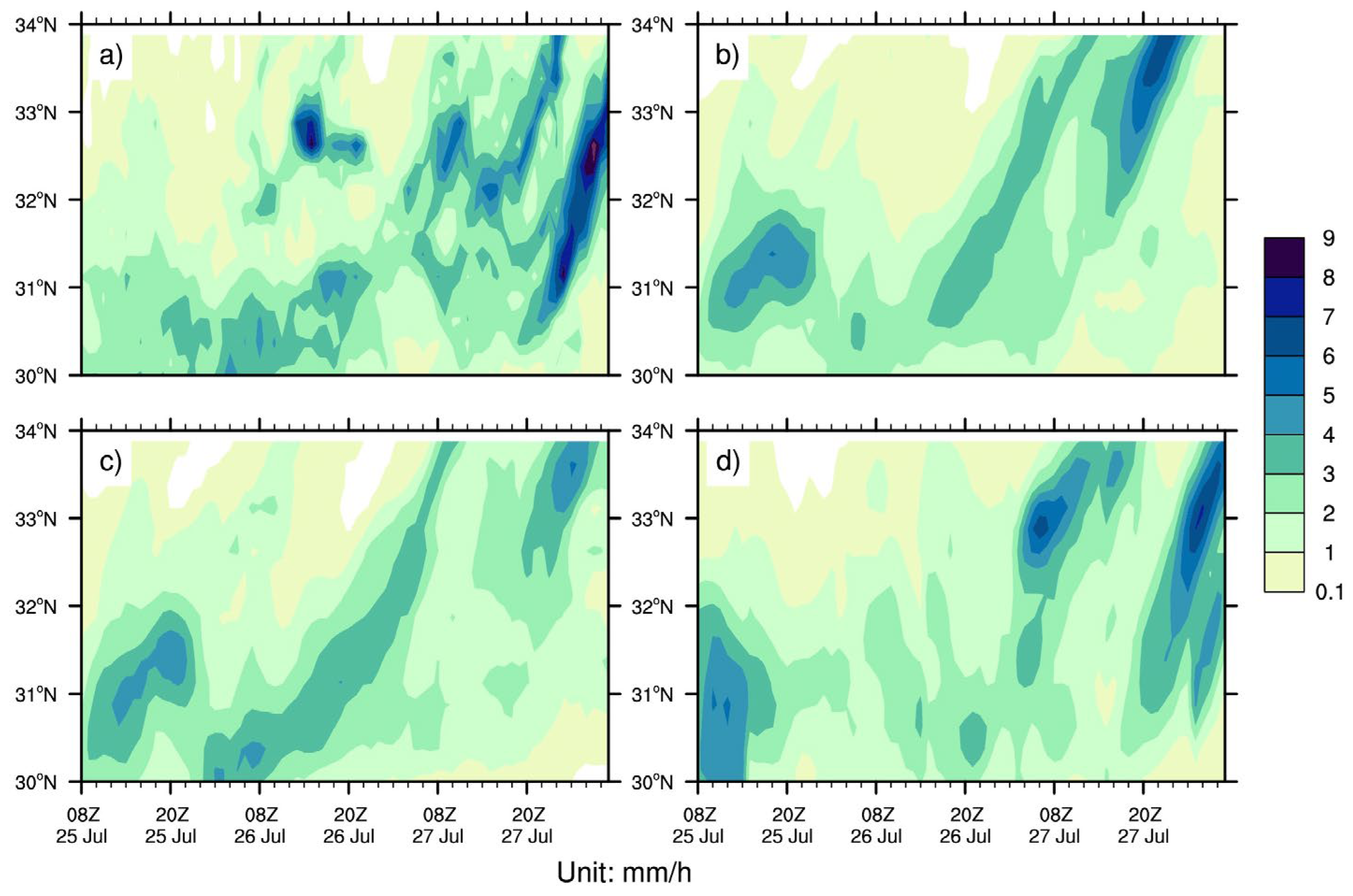
3.2. Influence of the Precipitation

To better describe the simulation bias distribution, we use the relative bias method to express, which is shown in Equation (22)

$$R_{bias}=\frac{P_{simulation}-P_{observation}}{P_{observation}}\times 100\mathrm{\%}.$$

(22)

The accumulated precipitation simulation of the CTL-25d experiment is shown in Figure 2b, ranged from 08 BT 25 July to 08 BT 28 July, with the severe rainfall concentrates north of In-Fa’s landfall areas while the observation distributions at the north and the south of the landfall area and another precipitation center is located at around (119° E, 30–32° E), which the simulation of the CTL-25d is absent. The modified scheme’s experiment (GWD-25d, Figure 2c) increases precipitation south of In-Fa’s landfall region and rainfall around the 119° E areas, which is closer to ERA5 reanalysis data (Figure 2d). The bias distribution (Figure 3c) shows that the black spots, which denote the errors reduced by above 25 mm, are dominantly located the south of Hangzhou Bay and around the 119° E region. A similar distribution is also represented in Figure 3d, which denotes that the relative bias is significantly reduced (above 10%) in the above region. The results simulated using the 0.125° model are similar to those of the 0.25° simulation.

Figure 4b,c show the hourly precipitation simulation of the model with a horizontal of 0.25°. The CTL-25d significantly overestimated precipitation exceeding 4 mm h⁻¹ in the 30.5°–32° N region before the In-Fa landfall period. In comparison, the GWD-25d decreases the bias by reducing the occurrence area of overestimated precipitation beyond 4 mm h⁻¹. The CTL-25d also underestimated precipitation in the 30°–31° N region after the landfall period, simulating only 2–3 mm h⁻¹ while the observation exceeded 4 mm h⁻¹. The GWD-25d experiment increases the precipitation in this region, effectively reducing the bias in the CTL-25d and producing rainfall amounts beyond 4 mm h⁻¹, closer to the observation. Compared with the corresponding time of ERA5 reanalysis (Figure 4d), the GWD-25d produces hourly precipitation intensity closer to the observations at the southern region of the “In-Fa”’s landfall (30°–31° N), which the ERA5 results are only 1–2 mm h⁻¹. It indicates that around the typhoon landfall, the GWD-25d improves the accumulated precipitation and the simulated temporal distribution of the precipitation. Therefore, the period of 08 (BT)–14 (BT) on 25 July, before Typhoon In-Fa made landfall, and 03 (BT)–06 (BT) on 26 July after landfall is selected for analysis of the accumulated precipitation as Figure 5 and Figure 6 shown.

Figure 5 denotes simulated precipitation from the CTL-25d and the GWD-25d experiments compared with the observation around the Typhoon In-Fa landfall. The observation shows the severe storm located south of Hangzhou Bay with 28°–30° N, while the CTL-25d underestimated the rainfall, as shown in Figure 5b. Another severe precipitation center, beyond 20 mm, from the observation is located at the (118°–120° E, 30–31° N), while the simulated precipitation also represents the underestimated bias with around 5 mm. The CTL-25d simulated precipitation shows the overestimated bias north of Hangzhou Bay by increasing above 10 mm during the period, while the range of the severe precipitation from observation is narrow. The observation also denotes the light rain region at (119° E, 31°–32.5° N) with a value of 0.1–2 mm, while the simulation from CTL-25d with 5–10 mm. The GWD-25d with the modified scheme reduces the above underestimated and overestimated rainfall biases. The black spots in Figure 5d,f represent the decreased bias above 5 mm and 40%. The precipitation with the GWD-25d experiment south of Hangzhou Bay increases by 2–6 mm, and the simulated precipitation from the rainfall center at (119° E, 31°–32.5° N) is also enforced with a reduced 40% bias. The precipitation bias with GWD-25d north of Hangzhou Bay is also reduced by 2–6 mm, and the light rain region with 0.1–2 mm is enlarged with the GWD-25d experiment. Figure 6 indicates the precipitation distribution with the period of Typhoon In-Fa’s northward movement. The precipitation centers from the observation are located south and north of Hangzhou Bay at (30°–31° N), the center of the study region (117°–119° E, 30°–31° N) with above 15 mm rainfall, and the two rain belts extended northward from this region with the value above 10 mm. The simulated precipitation from the CTL-25d is weaker compared with the observation, especially east of the 118° E. The simulation from the CTL-25d slightly increases the north of Hangzhou Bay with the rainfall center northwards; the precipitation at other rainfall centers is underestimated with the value of about 2–5 mm, and the northwards rain belts with the CTL-25d are not shown very clearly. The modified simulation from the GWD-25d increases precipitation south and north of Hangzhou Bay, and it also forms two northward rain bands beyond 10 mm with a location west than the observation compared to the nearly absent simulation from the CTL-25d experiment. Figure 5 and Figure 6 indicate that the modified gravity wave drag of the simulated precipitation shows the improved rainfall location before and after the Typhoon In-Fa landfall.

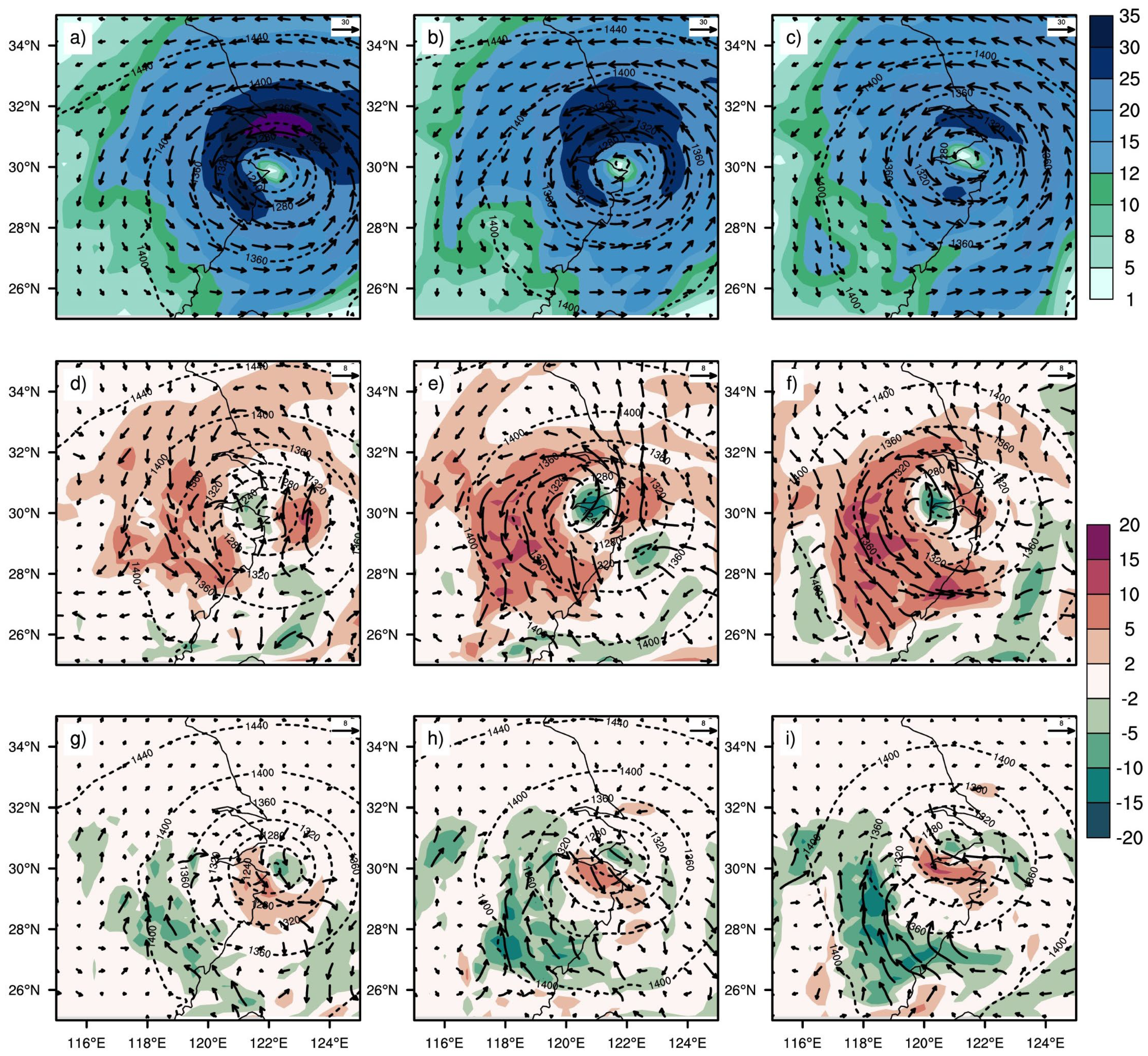
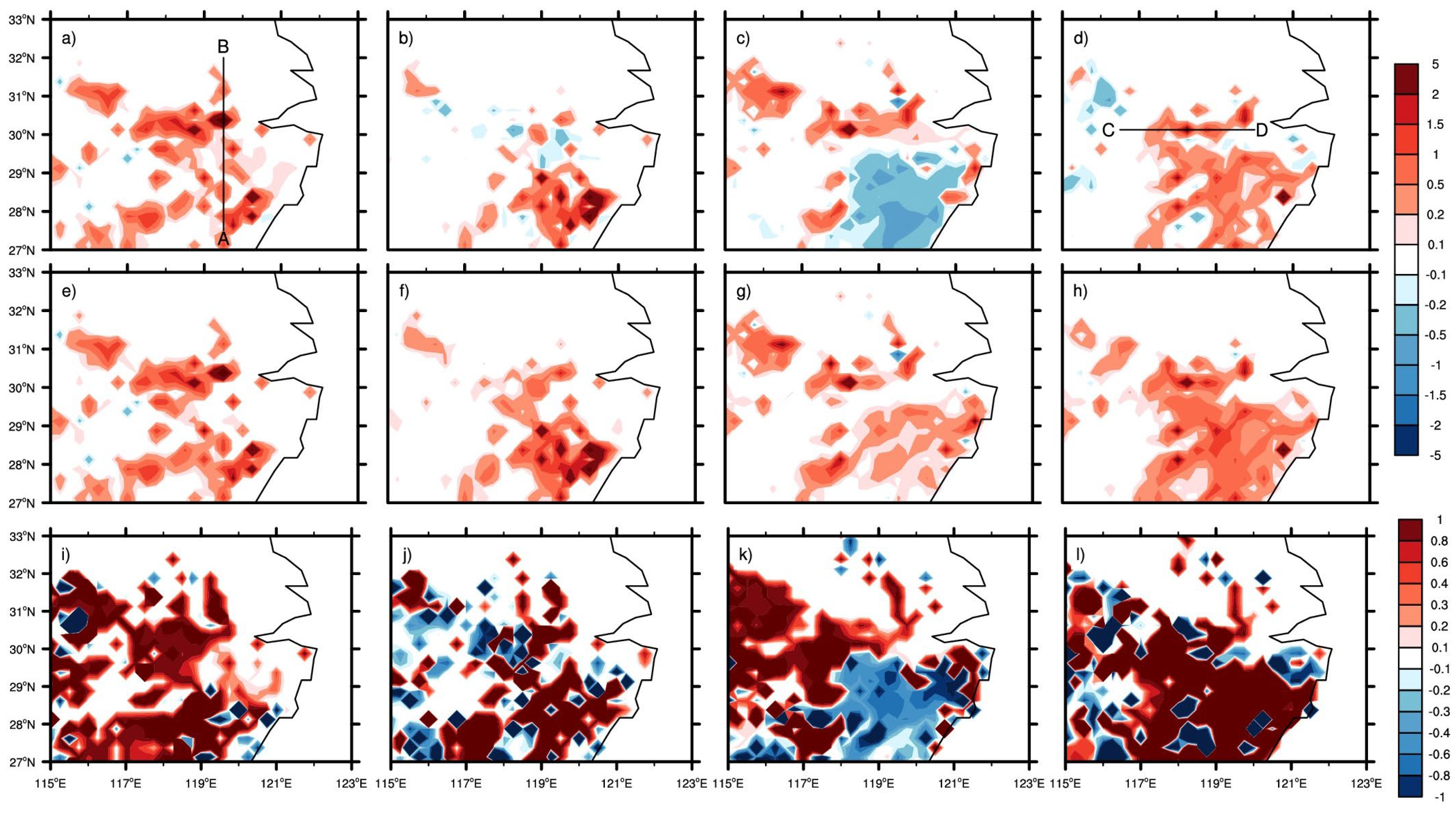
3.3. Influence of the Winds

The 850 hPa horizontal wind field, wind speed, and geopotential height correspond to the two severe precipitation events of Section 3.2, illustrated in Figure 7. The horizontal wind speed of 850 hPa around Typhoon In-Fa landfall derived from ERA5 shows the region of maximum wind speed beyond 30 m s⁻¹ concentrates at the west and north of the Typhoon center (Figure 7a). The simulation bias of the CTL-25d (Figure 7d) represents an overestimated wind speed west and north of the Typhoon center with a value beyond 5–10 m s⁻¹. The circulation at the low level of the troposphere of the CTL-25d shows stronger cyclonic circulation because the wind field’s bias describes the southward and eastward. The wind speed simulation of the GWD-25d (Figure 7g) helps to reduce the overestimated error, especially in the south of the region, by the value of 5–10 m s⁻¹.

In the 6 h following the typhoon’s landfall (Figure 7b) and in the early morning of the next day (Figure 7c), according to ERA5 data, the area with wind speeds beyond 30 m s⁻¹ at 850 hPa decreases over time. The CTL-25d simulation overestimated wind speeds on the west side of the typhoon center at both times, with biases of 5–10 m s⁻¹ and locally exceeding 10–15 m s⁻¹ shown in Figure 7e,f. Moreover, the errors in wind speeds of the low-level troposphere increase as time progresses. Compared to the CTL-25d, the GWD-25d simulation (Figure 7h,i) shows a reduction in the overestimated area, with values around 5–10 m s⁻¹. By the early morning of the next day, the simulation of the GWD-25d reduces the wind speed with the value of 10–15 m s⁻¹, aligning more closely with the ERA5 data. At the time of the landfall, 6 h after the landfall, and the early morning of the next day, the minimum wind speed centers in the CTL-25d simulation are located slightly westward compared to ERA5. The locations of the minimum wind speed centers of the GWD-25d are also close to ERA5 reanalysis data, with the simulations shifting slightly eastward compared to the CTL-25d simulation. It indicates that the modified gravity wave drag can help alleviate the location bias of the Typhoon center.

The 500 hPa and 200 hPa wind speed distributions at the three corresponding times are shown in Figure 8 and Figure 9. The areas with maximum wind speeds exceeding 30 m s⁻¹ shrinks and eventually disappear over time. The simulation of the CTL-25d overestimates the wind speed at 500 hPa (Figure 8e,f) and 200 hPa (Figure 9e,f) 6 h after landfall and early morning of the next day, respectively, while the simulation of the GWD-25d shows a slight improvement in the wind speed. The cyclonic circulation in the CTL-25d is westward-biased, while the bias is alleviated in the GWD-25d results. Although the improvement in wind field biases is slight of the GWD-25d at the middle and top levels of the troposphere, the 200 hPa geopotential height is improved (Figure 9h,i), strengthening the underestimated height field in the CTL-25d. The westward extensions of the 12,540 m and 12,530 m contours 6 h after landfall and early morning of the next day are closer to the ERA5 reanalysis data with the GWD-25d.

The results of the 0.125° simulation of the wind field at 850 hPa are similar to the 0.25° experiments. Since the simulation of precipitation and wind field of 0.125° are consistent with those of the 0.25°, and at the meantime, the horizontal scale of the gravity waves is 1–10 km, 0.125° is close to resolving the partly of them, while 0.25° allows the model to parameterize the subgrid-scale effects of gravity waves. Hence, we focus on analyzing the simulation of the 0.25° experiments (the CTL-25d and the GWD-25d).

Corresponding to the accumulated precipitation during the typhoon landfall, the integrated water vapor transport divergence presents convergence associated with severe precipitation and divergence with light rain in Figure 10. The simulation from the GWD-25d demonstrates that the convergence is more intense on the southern side of Typhoon In-Fa’s landfall area compared to the CTL-25d simulation (Figure 10e). A strong convergence region also emerges near 120° E, corresponding to the stronger precipitation simulated using the GWD-25d compared to the CTL-25d during the In-Fa landfall. Meanwhile, on the northern side of In-Fa landfall, moisture divergence shown in the GWD-25d simulation, compared to the CTL-25d, also corresponds to the reduction in the simulation of the CTL-25d overestimation of precipitation in the regions, bringing it closer to the observations. During the early morning of the next day, the vertical integration of the divergence water vapor transport of the GWD-25d at the area (119–121° E, 30–31° N) exhibits a stronger convergence, corresponding to the increased precipitation simulation where in the CTL-25d underestimation region.

Figure 11 illustrates the changes in the wind stress induced by the total gravity wave drag process, which includes the FBD effect, with the modified gravity wave drag scheme during and after the In-Fa landfall. The changes in u-component wind stress are predominantly increases, with the maximum value exceeding 2 N m⁻², while the negative region of the differences in u-wind stress (Figure 11c) corresponds to the increasing easterly winds in the GWD-25d compared to the CTL-25d in the early morning in the next day after landfall (Figure 7i), which belongs to the wind direction alteration. The changes in the v-component wind stresses are also increased. In the study area’s southern hilly and mountainous regions, the changes in wind stress for both u and v wind stress fields due to the FBD effect are around 0.5–1 N m⁻², with the maximum values of 2–5 N m⁻². The changes brought by the modified gravity wave drag scheme primarily increase due to the enhanced FBD effects, contributing over 80% of the total changes in the GWD process. Two regions, “A–B” and “C–D,” have been selected to investigate the changes in the u-wind and v-wind fields and vertical velocity during and after In-Fa landfall, as shown in Figure 12.

The changes in wind stress can lead to differences in the horizontal-vertical wind circulation. Figure 12 displays the distribution of wind field differences in regions with significant wind stress changes during and after landfall. During the landfall of In-Fa, at the low-level troposphere, the changes in v-wind due to the increased FBD effect resulted in the vertical velocity, producing the alternating distribution of ascending and descending motions with latitude, particularly near the vicinity of the maximum subgrid orography where the maximum vertical velocity exceeding 6 cm s⁻¹, corresponding to the increased precipitation regions in Figure 5f. After In-Fa landfall, from the low-level and the high-level of the troposphere, an extensive area of ascent occurs at the east of 119° E, with the maximum values exceeding 10 cm s⁻¹ and the influence reaching up to around 200 hPa. The spatial distribution of the differences in the ascending area is related to the increased precipitation in Figure 6f. Although the FBD effect primarily impacts the low-level troposphere, changes in the horizontal winds and wind directions led to impacts on the vertical motion, subsequently influencing the precipitation simulation.

The differences in the horizontal wind simulations caused by different model resolutions are shown in Figure 13. According to Niekerk and Vosper’s study, as the model grid spacing decreases, the influence of high-resolution terrain on the model can be more accurately expressed, but most of the current gravity wave drag parameterization schemes used in models are insensitive to changes in the model’s horizontal resolution. Similar to most current models that have not updated their gravity wave drag scheme, the CMA-GFS also shows only a weak impact on the low-level flow when the resolution changes from 0.25° to 0.125°, with changes mostly below 1 m s⁻¹ d⁻¹ over most areas (Figure 13a,c). Via the modified gravity wave drag scheme, especially considering the treatment of the maximum of the subgrid-scale orography varying with the subgrid orography standard deviation, producing the changes exceeding 3 m s⁻¹d⁻¹, becomes more sensitive to the resolution changes (Figure 13b,d), which is more reasonable.

3.4. Medium-Range Forecast Results

To evaluate the impact of the gravity wave drag parameterization, the CTL-25d was used as the control experiment, and the GWD-25d was used as the modified experiment to conduct an 8-day forecast daily from 1 July to 31 July 2021. The results are statistically analyzed to examine the changes induced by the modification of the gravity wave drag scheme. For the observation data and forecast results, the standard deviation error ($\mathsf{\sigma }$) between the forecast results and the observed data is defined as

$${\mathsf{\sigma }}^2=\frac{1}{n-1}\sum _{i=1}^n{\left[\left({\mathrm{X}}_i-{\mathrm{Y}}_i\right)-(\overline{X}-\overline{Y})\right]}^2,$$

(23)

and the confidence interval of the differences between the two datasets is defined as $\left[\left(\overline{X}-\overline{Y}\right)-t_{\raisebox{1ex}{$\alpha $}\!\left/ \!\raisebox{-1ex}{$2$}\right.}\left(\sqrt{\frac{{\mathsf{\sigma }}^2}{n}}\right),\left(\overline{X}-\overline{Y}\right)+t_{\raisebox{1ex}{$\alpha $}\!\left/ \!\raisebox{-1ex}{$2$}\right.}\left(\sqrt{\frac{{\mathsf{\sigma }}^2}{n}}\right)\right].$ For the 95% confidence level test, $\alpha =0.05$ means that the average deviation of the experiment results in 95% falls within the confidence interval [42]. Figure 14, Figure 15 and Figure 16 (the bottom panel) display whether the forecast results pass the 95% confidence level test, which indicates the statistical significance of the experiment results.

Figure 14 displays the equitable threat scores for 24 h accumulated precipitation forecasts over the mainland of China. The statistics score indicates a significant enhancement in the simulation using the improved gravity wave drag scheme experiment within the ranges of 0.1 mm, 1 mm, and above 100 mm, along with an enhancement in the precipitation of 25 mm rainfall intensity compared with the control experiment. This implies that the updated gravity wave drag experiment is beneficial for simulating precipitation bands above 0.1 mm and the intense precipitation of large magnitude effectively. The refined scheme also impacts the simulation of near-surface variables. The root mean square error (RMSE) of the 2 m temperature across mainland China (Figure 15) demonstrates a significant reduction within the 72 h forecast with the updated gravity wave drag scheme compared to the control run. The RMSE of the 10 m wind field (Figure 16) displays a statistically significant decrease in consistency with the forecast length of 0–192 h integration. Compared with EC’s forecast, the modified experiment (the GWD-25d) has a higher ETS score than EC’s forecast for precipitation above 0.1 mm. Although there is an improvement over the CTL-25d experiment, there still remains a gap in the scores above 1 mm compared to EC’s forecast. The simulation with the improvement in the gravity wave drag scheme of the RMSE of 2 m temperature is closer to the EC forecast within 96 h forecast, and the RMSE for 10m wind in the GWD-25d simulation with the lead time between 24–120 h is comparable to that of the EC’s forecast. The results of the medium-range forecast suggest that the adoption of the improved gravity wave drag scheme not only significantly improves the simulations of the near-surface variables but also enhances the simulation of precipitation bands and intense precipitation amounts effectively.

4. Conclusions and Discussion

The gravity wave drag process is crucial for the numerical weather forecast of the atmospheric circulation, particularly impacting the wind fields in both the low-level and upper-level troposphere. However, there are uncertainties in the traditional gravity wave drag parameterization schemes. Research indicates that differing processing schemes result in varied subgrid scale gravity wave drag influences even with the exact horizontal resolution. This study introduces a Fourier transformation method to employ an effective subgrid-scale orography in the gravity wave drag, allowing the maximum subgrid orography to involve the variance effect of its standard deviation replacing the traditional scheme’s elliptical assumption suited for isolated mountains under ideal conditions that lead to producing uncertainties in the scheme. When considering the FBD effect, the calculation of the dividing streamline height has been modified, thereby improving the intensity of the gravity wave drag effect caused by the FBD effect. This study analyzes the heavy rainfall event during and after the landfall of Typhoon In-Fa in Zhejiang Province and diagnoses the impacts of the improved gravity wave parameterization scheme over the continuous hilly regions of southwestern Zhejiang Province with the CMA-GFS numerical weather forecasting system.

This study mainly investigates the period during which Typhoon In-Fa moves slowly over Hangzhou Bay. The refined gravity wave drag parameterization scheme helps in enhancing the underestimated precipitation simulated using the CTL-25d, the control experiment, on the southern region of the typhoon center. Simultaneously, the GWD-25d, with the updated gravity wave drag scheme, produces an intense precipitation center in the western area of the typhoon’s center that the CTL-25d fails to simulate. Compared with the CTL-25d, the GWD-25d with the refined scheme reduces the precipitation bias by 25 mm and relative bias by 10% in most areas of the study region, which is closer to the ERA5 reanalysis and the observation. The improved scheme also enhanced hourly precipitation simulations, which is beneficial in alleviating the overestimated precipitation during Typhoon In-Fa’s landfall and producing the intense precipitation generated when Typhoon In-Fa was moving slowly in Hangzhou Bay, which is absent in the CTL-25d and ERA5 reanalysis. By diagnosing the accumulated precipitation during and after the landfall of Typhoon In-Fa, it is evident that the refined scheme significantly reduces both the bias and relative bias in precipitation simulation. The intensity and region distribution of precipitation are close to the observation in the updated scheme.

The improved gravity wave drag scheme primarily impacts the simulation of the low-level wind fields in the troposphere. Compared with ERA5 reanalysis, the improved scheme effectively reduces the overestimated wind speed at 850 hPa in the CTL-25d, weakens the cyclonic circulation on the western side of the typhoon center, and aids in improving the simulation of the typhoon center location. The wind speed biases in the middle and upper troposphere are also reduced, which is beneficial for simulating the upper-level geopotential height. Compared to the CTL-25d, the GWD-25d produces a stronger convergence of the integrated water vapor transport on the southern and western sides of the landfall and stronger divergence on the northern side, correlating with the improvement in precipitation forecast bias. The improved scheme increased the column-integrated horizontal wind stress, with a general increase of 0.5 N m⁻¹ in the study region, with the influence caused by FBD accounting for over 80% of the total gravity wave drag effect. The vertical cross-sections of horizontal wind and vertical velocity show that in regions with large wind stress changes, the GWD-25d helps to enhance ascending motions related to the reduced precipitation biases. The CTL-25d displays the insensitive parameterized horizontal wind tendencies at low-level troposphere with different resolutions of 0.125° and 0.25°, while the GWD-25d displays a more sensitive effect of gravity wave drag at different resolutions, aligning more closely with reality.

The medium-range forecast results indicate that the GWD-25d effectively enhances the precipitation score of light rain and heavy storm precipitation. The ETS score is even higher than the EC’s forecast beyond 0.1 mm. Additionally, there is a significant improvement in reducing the RMSEs for both 2 m temperature, which is closer to EC’s forecast, and 10 m wind, which is comparable to the EC’s forecast.

As the horizontal resolution improves, whether the process of gravity wave drag can be uniformly parameterized across horizontal scales is a crucial question in numerical weather prediction models. The parameterization of gravity wave drag across horizontal model scales is a complex task. The concept proposed by Nierkerk [13] avoided the traditional idealized elliptical assumption. They proposed an approach to solve for the corresponding Fourier transform coefficients directly from high-resolution models. This study has modified the influential parameters of subgrid-scale orography and dividing streamline height. These changes affect the wind field and speed in the lower troposphere, as well as the wind stress and the associated ascending and descending motions, and the divergence of the integrated water vapor transport. Consequently, these modifications have enhanced the performance of the model’s precipitation forecast. However, we have not applied the full complicated Fourier transform scheme to diagnose the impacts, especially for China. The unique terrain of East Asia, including the Tibetan Plateau, suggests that the gravity wave drag process could potentially influence the downstream circulation patterns and precipitation simulations. This potential impact warrants further investigation in future work. Along with the effects of turbulent orographic form drag process with horizontal resolution enhancement, impacting atmospheric circulation and even precipitation simulation will be investigated in the following study.

References

1. Sandu, I.; Van Niekerk, A.; Shepherd, T.G.; Vosper, S.B.; Zadra, A.; Bacmeister, J.; Beljaars, A.; Brown, A.R.; Dörnbrack, A.; McFarlane, N.; et al. Impacts of Orography on Large-Scale Atmospheric Circulation. Npj Clim. Atmos. Sci. 2019, 2, 10. [Google Scholar] [CrossRef]
2. Teixeira, M.A.C. The Physics of Orographic Gravity Wave Drag. Front. Phys. 2014, 2, 43. [Google Scholar] [CrossRef]
3. Tsiringakis, A.; Steeneveld, G.J.; Holtslag, A.A.M. Small-Scale Orographic Gravity Wave Drag in Stable Boundary Layers and Its Impact on Synoptic Systems and near-Surface Meteorology: Orographic Gravity Wave Drag in Stable Boundary Layers. Q. J. R. Meteorol. Soc. 2017, 143, 1504–1516. [Google Scholar] [CrossRef]
4. Van Niekerk, A.; Sandu, I.; Vosper, S.B. The Circulation Response to Resolved Versus Parametrized Orographic Drag Over Complex Mountain Terrains. J. Adv. Model. Earth Syst. 2018, 10, 2527–2547. [Google Scholar] [CrossRef]
5. Elvidge, A.D.; Sandu, I.; Wedi, N.; Vosper, S.B.; Zadra, A.; Boussetta, S.; Bouyssel, F.; Niekerk, A.; Tolstykh, M.A.; Ujiie, M. Uncertainty in the Representation of Orography in Weather and Climate Models and Implications for Parameterized Drag. J. Adv. Model. Earth Syst. 2019, 11, 2567–2585. [Google Scholar] [CrossRef]
6. Van Niekerk, A.; Sandu, I.; Zadra, A.; Bazile, E.; Kanehama, T.; Köhler, M.; Koo, M.; Choi, H.; Kuroki, Y.; Toy, M.D.; et al. COnstraining ORographic Drag Effects (COORDE): A Model Comparison of Resolved and Parametrized Orographic Drag. J. Adv. Model. Earth Syst. 2020, 12, e2020MS002160. [Google Scholar] [CrossRef]
7. Vosper, S.B.; Van Niekerk, A.; Elvidge, A.; Sandu, I.; Beljaars, A. What Can We Learn about Orographic Drag Parametrisation from High-resolution Models? A Case Study over the Rocky Mountains. Q. J. R. Meteorol. Soc. 2020, 146, 979–995. [Google Scholar] [CrossRef]
8. Wang, Y.; Yang, K.; Zhou, X.; Chen, D.; Lu, H.; Ouyang, L.; Chen, Y.; Lazhu; Wang, B. Synergy of Orographic Drag Parameterization and High Resolution Greatly Reduces Biases of WRF-Simulated Precipitation in Central Himalaya. Clim. Dyn. 2020, 54, 1729–1740. [Google Scholar] [CrossRef]
9. Rodrigues Gonçalves, M.; Rozenman, G.G.; Zimmermann, M.; Efremov, M.A.; Case, W.B.; Arie, A.; Shemer, L.; Schleich, W.P. Bright and Dark Diffractive Focusing. Appl. Phys. B 2022, 128, 51. [Google Scholar] [CrossRef]
10. Arbic, B.K. Incorporating Tides and Internal Gravity Waves within Global Ocean General Circulation Models: A Review. Prog. Oceanogr. 2022, 206, 102824. [Google Scholar] [CrossRef]
11. Williams, E.F.; Zhan, Z.; Martins, H.F.; Fernández-Ruiz, M.R.; Martín-López, S.; González-Herráez, M.; Callies, J. Surface Gravity Wave Interferometry and Ocean Current Monitoring with Ocean-Bottom DAS. JGR Ocean. 2022, 127, e2021JC018375. [Google Scholar] [CrossRef]
12. Rozenman, G.G.; Zimmermann, M.; Efremov, M.A.; Schleich, W.P.; Case, W.B.; Greenberger, D.M.; Shemer, L.; Arie, A. Projectile Motion of Surface Gravity Water Wave Packets: An Analogy to Quantum Mechanics. Eur. Phys. J. Spec. Top. 2021, 230, 931–935. [Google Scholar] [CrossRef]
13. Van Niekerk, A.; Vosper, S.B. Towards a More “Scale-aware” Orographic Gravity Wave Drag Parametrization: Description and Initial Testing. Q. J. R. Meteorol. Soc. 2021, 147, 3243–3262. [Google Scholar] [CrossRef]
14. Feng, L.; Zhang, Y. Impacts of the Thermal Effects of Sub-Grid Orography on the Heavy Rainfall Events along the Yangtze River Valley in 1991. Adv. Atmos. Sci. 2007, 24, 881–892. [Google Scholar] [CrossRef]
15. Choi, H.-J.; Hong, S.-Y. An Updated Subgrid Orographic Parameterization for Global Atmospheric Forecast Models: Subgrid Orographic Parameterization. J. Geophys. Res. Atmos. 2015, 120, 12445–12457. [Google Scholar] [CrossRef]
16. Zhong, S.; Chen, Z. Improved Wind and Precipitation Forecasts over South China Using a Modified Orographic Drag Parameterization Scheme. J. Meteorol. Res. 2015, 29, 132–143. [Google Scholar] [CrossRef]
17. Zhang, R.; Xu, X.; Wang, Y. Impacts of Subgrid Orographic Drag on the Summer Monsoon Circulation and Precipitation in East Asia. JGR Atmos. 2020, 125, e2019JD032337. [Google Scholar] [CrossRef]
18. Deng, L.; Feng, J.; Zhao, Y.; Bao, X.; Huang, W.; Hu, H.; Duan, Y. The Remote Effect of Binary Typhoon Infa and Cempaka on the “21.7” Heavy Rainfall in Henan Province, China. JGR Atmos. 2022, 127, e2021JD036260. [Google Scholar] [CrossRef]
19. Wang, L.; Gu, X.; Slater, L.J.; Lai, Y.; Zhang, X.; Kong, D.; Liu, J.; Li, J. Indirect and Direct Impacts of Typhoon In-Fa (2021) on Heavy Precipitation in Inland and Coastal Areas of China: Synoptic-Scale Environments and Return Period Analysis. Mon. Weather. Rev. 2023, 151, 2377–2395. [Google Scholar] [CrossRef]
20. Yang, S.; Chen, B.; Zhang, F.; Hu, Y. Characteristics and Causes of Extremely Persistent Heavy Rainfall of Tropical Cyclone In-Fa (2021). Atmosphere 2022, 13, 398. [Google Scholar] [CrossRef]
21. Sun, Z. The Extraordinarily Large Vortex Structure of Typhoon In-Fa (2021), Observed by Spaceborne Microwave Radiometer and Synthetic Aperture Radar. Atmos. Res. 2023, 292, 106837. [Google Scholar] [CrossRef]
22. Wu, Z.; Zhang, Y.; Zhang, L.; Zheng, H.; Huang, X. A Comparison of Convective and Stratiform Precipitation Microphysics of the Record-Breaking Typhoon In-Fa (2021). Remote Sens. 2022, 14, 344. [Google Scholar] [CrossRef]
23. Huang, X.; Chan, J.C.L.; Zhan, R.; Yu, Z.; Wan, R. Record-breaking Rainfall Accumulations in Eastern China Produced by Typhoon In-fa (2021). Atmos. Sci. Lett. 2023, 24, e1153. [Google Scholar] [CrossRef]
24. Yu, Y.; Gao, T.; Xie, L.; Zhang, R.-H.; Zhang, W.; Xu, H.; Cao, F.; Chen, B. Tropical Cyclone over the Western Pacific Triggers the Record-Breaking ‘21/7’ Extreme Rainfall in Henan, Central-Eastern China. Environ. Res. Lett. 2022, 17, 124003. [Google Scholar] [CrossRef]
25. Rao, C.; Chen, G.; Ran, L. Effects of Typhoon In-Fa (2021) and the Western Pacific Subtropical High on an Extreme Heavy Rainfall Event in Central China. J. Geophys. Research. 2023, 128, e2022JD037924. [Google Scholar] [CrossRef]
26. Liu, L.; Ran, L.; Sun, X. Analysis of the Structure and Propagation of a Simulated Squall Line on 14 June 2009. Adv. Atmos. Sci. 2015, 32, 1049–1062. [Google Scholar] [CrossRef]
27. Zhuang, Y. Failure and Disaster-Causing Mechanism of a Typhoon-Induced Large Landslide in Yongjia, Zhejiang, China. Landslides 2023, 20, 2257–2269. [Google Scholar] [CrossRef]
28. Wu, M.; Dong, M.; Chen, F.; Yu, Z.; Luo, Y. A Comparison of Different Station Data on Revealing the Characteristics of Extreme Hourly Precipitation Over Complex Terrain: The Case of Zhejiang, China. Earth Space Sci. 2023, 10, e2023EA002925. [Google Scholar] [CrossRef]
29. Huang, B.; Chen, D.; Li, X.; Li, C. Improvement of the Semi-Lagrangian Advection Scheme in the GRAPES Model: Theoretical Analysis and Idealized Tests. Adv. Atmos. Sci. 2014, 31, 693–704. [Google Scholar] [CrossRef]
30. Chen, D.; Xue, J.; Yang, X.; Zhang, H.; Shen, X.; Hu, J.; Wang, Y.; Ji, L.; Chen, J. New Generation of Multi-Scale NWP System (GRAPES): General Scientific Design. Sci. Bull. 2008, 53, 3433–3445. [Google Scholar] [CrossRef]
31. Mlawer, E.J.; Taubman, S.J.; Brown, P.D.; Iacono, M.J.; Clough, S.A. Radiative Transfer for Inhomogeneous Atmospheres: RRTM, a Validated Correlated-k Model for the Longwave. J. Geophys. Res. 1997, 102, 16663–16682. [Google Scholar] [CrossRef]
32. Han, J.; Pan, H.-L. Revision of Convection and Vertical Diffusion Schemes in the NCEP Global Forecast System. Weather. Forecast. 2011, 26, 520–533. [Google Scholar] [CrossRef]
33. Liu, K.; Chen, Q.; Sun, J. Modification of Cumulus Convection and Planetary Boundary Layer Schemes in the GRAPES Global Model. J. Meteorol. Res. 2015, 29, 806–822. [Google Scholar] [CrossRef]
34. Hong, S.-Y.; Pan, H.-L. Nonlocal Boundary Layer Vertical Diffusion in a Medium-Range Forecast Model. Mon. Wea. Rev. 1996, 124, 2322–2339. [Google Scholar] [CrossRef]
35. Ma, Z.; Liu, Q.; Zhao, C.; Li, Z.; Wu, X.; Chen, J.; Yu, F.; Sun, J.; Shen, X. Impacts of Transition Approach of Water Vapor-Related Microphysical Processes on Quantitative Precipitation Forecasting. Atmosphere 2022, 13, 1133. [Google Scholar] [CrossRef]
36. Dai, Y.; Zeng, X.; Dickinson, R.E.; Baker, I.; Bonan, G.B.; Bosilovich, M.G.; Denning, A.S.; Dirmeyer, P.A.; Houser, P.R.; Niu, G.; et al. The Common Land Model. Bull. Am. Meteorol. Soc. 2003, 84, 1013–1024. [Google Scholar] [CrossRef]
37. Kim, Y.-J.; Arakawa, A. Improvement of Orographic Gravity Wave Parameterization Using a Mesoscale Gravity Wave Model. J. Atmos. Sci. 1995, 52, 1875–1902. [Google Scholar] [CrossRef]
38. Lott, F.; Miller, M.J. A New Subgrid-Scale Orographic Drag Parametrization: Its Formulation and Testing. Q. J. R. Meteorol. Soc. 1997, 123, 101–127. [Google Scholar] [CrossRef]
39. Hersbach, H.; Bell, B.; Berrisford, P.; Hirahara, S.; Horányi, A.; Muñoz-Sabater, J.; Nicolas, J.; Peubey, C.; Radu, R.; Schepers, D.; et al. The ERA5 Global Reanalysis. Q. J. R. Meteorol. Soc. 2020, 146, 1999–2049. [Google Scholar] [CrossRef]
40. Good, S.; Fiedler, E.; Mao, C.; Martin, M.J.; Maycock, A.; Reid, R.; Roberts-Jones, J.; Searle, T.; Waters, J.; While, J.; et al. The Current Configuration of the OSTIA System for Operational Production of Foundation Sea Surface Temperature and Ice Concentration Analyses. Remote Sens. 2020, 12, 720. [Google Scholar] [CrossRef]
41. Shen, Y.; Zhao, P.; Pan, Y.; Yu, J. A High Spatiotemporal Gauge-Satellite Merged Precipitation Analysis over China. J. Geophys. Res. Atmos. 2014, 119, 3063–3075. [Google Scholar] [CrossRef]
42. Zhao, B.; Hu, J.; Wang, D.; Zhang, B.; Chen, F.; Wan, Z.; Sun, S. The GRAPES Evaluation Tools Based on Python (GetPy). CCF Trans. High Perform. Comput. 2022, 1–13. [Google Scholar] [CrossRef]
Figure 1. The distribution of (a) derived 30” GTOP30 terrain data, (b) grid-resolved terrain, (c) the subgrid-scale orography in CMA_GFS, and (d) the modified subgrid-scale orography (Unit: m).
Atmosphere 14 01801 g001
Figure 2. The precipitation distribution (Unit: mm) of the observation ((a) CMPAS), the CTL-25d (b), the GWD-25d (c), and ERA5 (d) with the entire period of Typhoon In-Fa landfall.
Atmosphere 14 01801 g002
Figure 3. The bias distribution (Unit: mm) between the CTL-25d (a) and observation, the GWD-25d and the observation (c), respectively, and the relative bias (Unit: %) between the CTL-25d (b) and the observation, the GWD-25d (d) and the observation, respectively. The black spots in the (c,d) denote the region of bias in GWD-25d reduced 25 mm (c) and 10% (d) compared to the CTL-25d.
Atmosphere 14 01801 g003
Figure 4. The latitude-time cross-section of hourly precipitation distribution averaged by (118°–122° E) of the CMPAS observation (a), the CTL-25d experiment (b), the GWD-25d experiment (c), and ERA5 (d) Unit: mm h−1.
Atmosphere 14 01801 g004
Figure 5. The accumulated precipitation distribution ranged by 08 (BT)–14 (BT) on 25 July from observation (a), the CTL-25d (c), and the GWD-25d (e); the bias distribution of the CTL-25d (b) and GWD-25d (d) from the observation and the difference (f) between the GWD-25d and the CTL-25d. The black spots in the (d,f) denote the region of bias in GWD-25d reduced 5 mm (d) and 40% (f) compared to the CTL-25d.
Atmosphere 14 01801 g005
Figure 6. The accumulated precipitation distribution ranged by 03(BT)–06(BT) on 26 July from observation (a), the CTL-25d (c), and the GWD-25d (e); the bias distribution of the CTL-25d (b) and GWD-25d (d) from the observation and the difference (f) between the GWD-25d and the CTL-25d. The black spots in the (d,f) denote the region of bias in GWD-25d reduced 5 mm (d) and 40% (f) compared to the CTL-25d.
Atmosphere 14 01801 g006
Figure 7. Horizontal wind speed (shading; unit: m s−1), wind field (arrow), and geopotential height (dash line, unit: m, with a contour interval of 40m) at 850 hPa for ERA5 reanalysis data from 14 (BT) 25 July (a), 20 (BT) 25 July (b), and 02 (BT) 26 July(c), respectively. The differences in horizontal wind speed and wind field between the CTL-25d and ERA5 are shown in (df). The differences between GWD-25d and CTL-25d are shown in (gi). The dash lines in (di) denote the simulated geopotential height from the CTL-25d and GWD-25d experiments.
Atmosphere 14 01801 g007
Figure 8. Horizontal wind speed and bias distribution (shading; unit: m s−1), wind field and bias (arrow), geopotential height (dash line, unit: m, with a contour interval of 40 m) at 500 hPa for ERA5 reanalysis data from 14 (BT) 25 July (a), 20 (BT) 25 July (b), and 02 (BT) 26 July (c), respectively. The differences in horizontal wind speed and wind field between the CTL-25d and ERA5 are shown in (df). The differences between GWD-25d and CTL-25d are shown in (gi). The dash lines in (di) denote the simulated geopotential height from the CTL-25d and GWD-25d experiments.
Atmosphere 14 01801 g008
Figure 9. Horizontal wind speed and bias distribution (shading; unit: m s−1), wind field and bias (arrow), geopotential height (dash line, unit: m, with a contour interval of 10 m) at 200 hPa for ERA5 reanalysis data from 14 (BT) 25 July (a), 20 (BT) 25 July (b), and 02 (BT) 26 July (c), respectively. The differences in horizontal wind speed and wind field between the CTL-25d and ERA5 are shown in (df). The differences between GWD-25d and CTL-25d are shown in (gi). The dash lines in (di) denote the simulated geopotential height from the CTL-25d and GWD-25d experiments.
Atmosphere 14 01801 g009
Figure 10. The vertical integrated (up to 100 hPa) horizontal wind field of the CTL-25d (vector, (a,b)) and the GWD-25d (vector, (c,d)) and the divergence of the integrated water vapor transport (shading, unit: kg m−2 s−1) averaged by 08 (BT)–14 (BT) 25 July and 03 (BT)–06 (BT) 26 July, respectively. The black lines denote the subgrid orography height (unit: m). The difference in the integrated wind field, the divergence of the water vapor transport, and the subgrid orography height between the GWD-25d and CTL-25d are shown in (e,f).
Atmosphere 14 01801 g010
Figure 11. The difference of the column-integrated horizontal wind stress (unit: N m−2) between the GWD-25d and the CTL-25d during In-Fa landfall averaged by 08 (BT)–14 (BT) 25 July (a,b,e,f), and 03 (BT)–06 (BT) 26 July (c,d,g,h), respectively. The difference of the u-component wind stress due to the total GWD (a,c) and due to the FBD (e,g) for the corresponding times, and the v-component wind stress difference due to the total GWD (b,d) and the FBD (f,h). The percentages of the wind stress changes caused by the FBD contributing to the GWD are shown in (il). The “A–B” and “C–D” denote the two areas (119.5° E, 27.5°–32° N), (116.5°–121° E, 30.125° N).
Atmosphere 14 01801 g011
Figure 12. Cross section of (a) the latitude-pressure of the difference in the v-wind (unit: m s−1) and vertical velocity w (shading, unit: 10−2 m s−1) averaged by 08 (BT)–14 (BT) 25 July between the GWD-25d and the CTL-25d, and (b) the longitude-pressure of the difference in the u-wind (unit: m s−1) and the vertical velocity w (shading, unit: 10−2 m s−1) averaged by 03 (BT)–06 (BT) 26 July between the GWD-25d and the CTL-25d, along the “A–B” and “C–D” lines denoted in Figure 11, respectively. The gray shaded areas indicate the maximum subgrid orography.
Atmosphere 14 01801 g012
Figure 13. The difference in the 24 h tendencies of the u-wind (a,b) and v-wind (c,d) is due to the gravity wave drag process at 850 hPa for the 0.125° and 0.25° models. The difference between the CTL-125d and the CTL-25d is shown in (a,c), and the difference between the GWD-125d and the GWD-25d is shown in (b,d). Unit is m s−1 d−1.
Atmosphere 14 01801 g013
Figure 14. Mean equitable threat score for 0–24 h precipitation forecasts over continental China (70°–145° E, 20°–55° N) for the control forecast (CTL-25d, the black bar), the modified scheme forecast (GWD-25d, the red bar), and EC’s forecast (the blue bar) averaged by 1 July to 31 July 2021. The bottom plot means significant at the 95% confidence level.
Atmosphere 14 01801 g014
Figure 15. Root mean square errors of 2 m temperature forecast over the mainland of China with lead times from 24 h to 192 h for the CTL-25d experiment (black line), the modified gravity drag scheme (GWD-25d, red line), and EC forecast (the blue line) experiment averaged by 1 July to 31 July 2021, Unit: K. The bottom plot means significant at the 95% confidence level.
Atmosphere 14 01801 g015
Figure 16. As in Figure 15, but root mean square errors of 10 m winds forecast over the mainland of China with the unit is m s −1.
Atmosphere 14 01801 g016