Numerical Analysis of SO₂ Absorption inside a Single Water Drop

Abstract

This paper introduces a numerical model dedicated to simulating SO₂ adsorption during the dynamic interplay between combustion gases and water droplets. The research delves into essential chemical–physical parameters governing mass transfer in these interphase interactions. The proposed simplified model provides preliminary results regarding the granulometric curve of sprays, particularly focusing on the minimal droplet size crucial for effective wet scrubber operation. Our findings underscore a critical diameter below which the spray loses its efficacy under varied boundary conditions. Notably, a single droplet with a maximum diameter of 2 mm absorbs more SO₂ than smaller counterparts, peaking at 4.36 × 10⁻⁵ g of SO₂ within the simulation timeframe. Furthermore, the study explores a specific water mass, revealing that smaller droplets, such as 1 mm, significantly optimize the absorption process. These droplets achieve a SO₂ absorption quantity over 5.77 times greater than that of a 2 mm droplet. This research serves as an initial tool for optimizing droplet distribution in sprays, thereby enhancing capture efficiency. The insights presented here offer valuable guidance for designing efficient wet scrubber systems, crucial for pollution control in industrial and environmental applications.

1. Introduction

Urban traffic stands as a major contributor to atmospheric pollutants like nitrogen oxides (NO_X) and particulate matter (PM) [1]. However, with the rise in international trade, pollution from marine sources could soon become as concerning as that from land-based sources [2]. While diesel engines on land have characteristic emissions, traditional marine engines emit not only those but also sulfur oxides (SO_X) due to the use of heavy fuels containing sulfur.

In response to this environmental challenge, the international community has been proactive in issuing directives to reduce emissions. The National Emissions reduction Commitments (NEC) Directive, in line with the 2020 Gothenburg protocol, focuses on reducing emissions into the air. Particularly, efforts have been made to address sulfur oxide emissions from exhaust gases, especially in marine applications. The 2016 EU environmental directive, first published in 1999 and last amended in 2012, emphasized reducing sulfur content in fuels, especially those used in naval contexts. This directive aligns with international developments under MARPOL Annex VI, setting a maximum limit of 0.50% m/m of sulfur in fuels. SO_X, the pollutant under consideration in this article, is directly impacted by these regulations.

To tackle SO_X emissions, Emission Control Areas (ECAS) have been established as part of the 2016 EU directive. Currently, four such areas exist under the MARPOL convention, with two of them located within the EU: the Baltic Sea area (MARPOL Annex I, 2006) and the North Sea area (MARPOL Annex VI, 2006). These initiatives make significant steps toward reducing sulfur oxide emissions from marine activities, a topic explored in this article.

Emission Control Areas (ECAs) are not limited to international directives; individual states can establish them to enhance the air quality in coastal regions and along inland rivers [3].

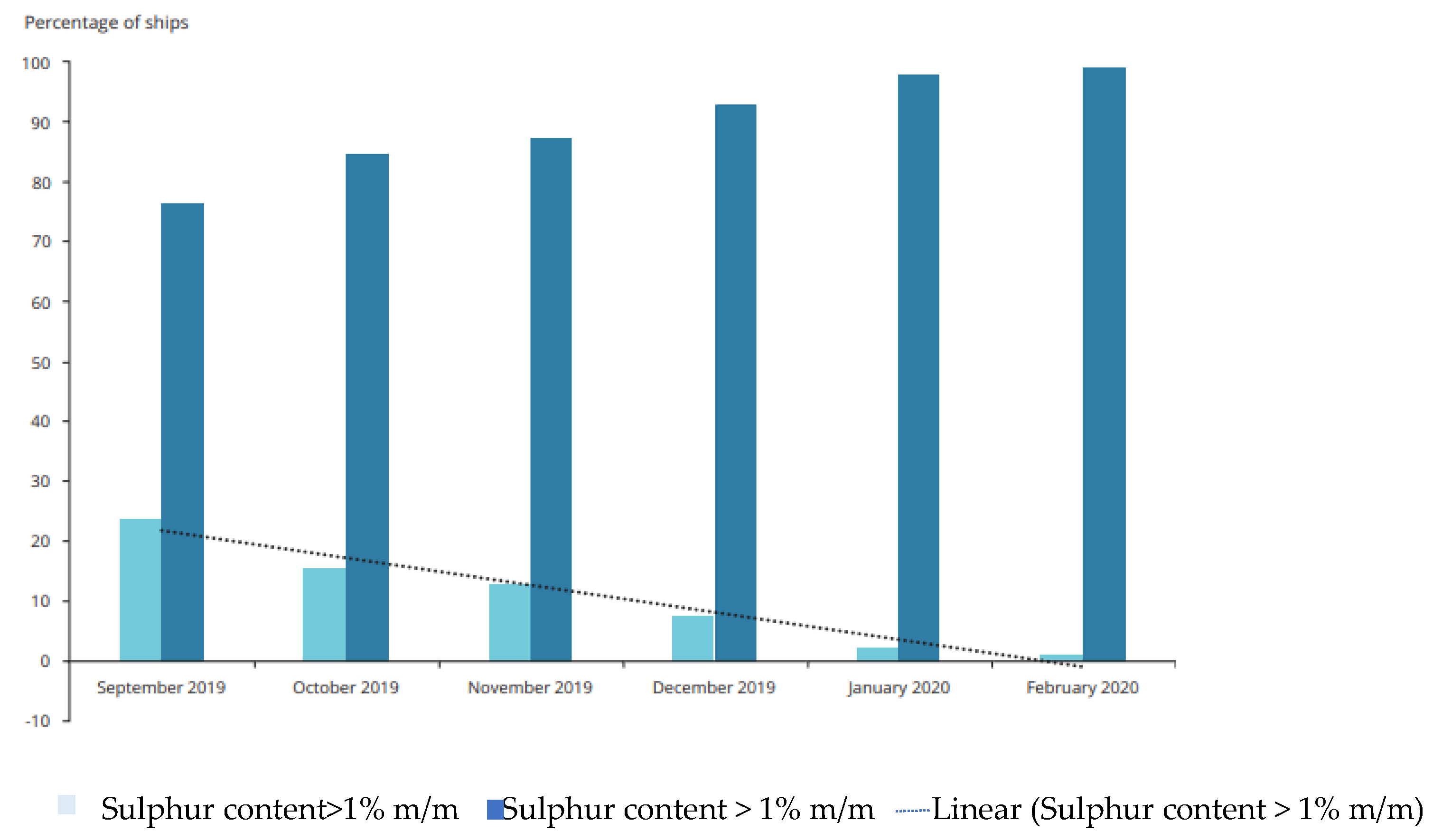
Furthermore, it is noteworthy that the percentage of ships using high-sulfur fuels has been consistently decreasing. In September 2019, 23.8% of ships were using high-sulfur fuels, a number that plummeted to 1.1% by February 2020. Conversely, there has been a significant surge in vessels opting for low-sulfur fuels (ranging from 0.10% to 0.50% m/m). This figure rose from 76.2% in September 2019 to encompass 98.9% of all vessels [3] (see Figure 1). These trends reflect a promising shift toward cleaner fuels and underscore the positive impact of regulatory measures on maritime emissions.

The ongoing transition to low-sulfur fuels necessitates the adaptation of naval units still employing high-sulfur fuels to comply with the MARPOL convention. To achieve this, vessels are required to equip themselves with sulphur abatement systems, such as wet scrubbers. The effectiveness of these systems hinges on the solubility of sulphur dioxide (SO₂) in water and its ability to form HSO₃ when bound to it [4].

An essential strategy to enhance SO₂ extraction from flue gases involves increasing the contact surface area between the gaseous and liquid phases [5]. This is typically achieved by injecting nebulized water into the exhaust gas stream. To optimize the SO₂ capture process, it is crucial to understand which droplet diameters are conducive to this process. Conversely, it is equally important to identify diameters that are not involved in SO₂ capture, once the thermodynamic conditions of the exhaust and the aqueous phase have been defined.

Researchers such as A. Tomaszewski and colleagues [6] have examined scrubber optimization by studying the impact of the number of demisters on particle removal efficiency. They also explored the probability of coalescence based on droplet size. Additionally, Jiarui Wang and collaborators employed genetic algorithms to optimize the interaction between scrubber geometry and droplet size distribution. R. Kaesemann and team [7] addressed not only droplet distribution but also the interaction between drops. Overlapping effects among drops can lead to coalescence, forming larger drops and altering effective diameter distribution. This dynamic phenomenon poses challenges to the optimization process.

Moreover, Kumaresh Selvakumar and colleagues [8] analyzed the interaction between drops and hot gas streams. They explored how water droplets absorbing SO₂ can significantly cool combustion gases due to their evaporation requirements. Controlling exhaust gas temperature offers another avenue for pollutant analysis and control.

It is crucial to note that optimizing a scrubber presents multifaceted challenges. Additionally, heavy-duty scrubbers have distinct optimization criteria in terms of dimensions (height and width) compared to scrubbers designed for naval applications. These complexities highlight the need for comprehensive research and innovative solutions in the realm of emission control systems.

Implementing water scrubbers for sulfur dioxide (SO₂) abatement poses challenges, especially due to space constraints, which are a concern for vessel owners. Therefore, optimizing water scrubbers remains an area of uncertainty. Researchers like Tibor Bešenić and colleagues [9] have explored the dynamic processes of water droplet evaporation and condensation when introduced into a known concentration stream of SO₂. Their work focused on understanding the interaction between water droplets and exhaust gases with known boundary conditions in terms of pressure, temperature, and relative speed. The study delved into diffusion mechanisms and chemical kinetics to simulate the absorption phenomenon and predict SO₂ absorption concentrations in individual water droplets. By analyzing droplet dynamics, the research identified the minimum diameters below which droplets contribute insignificantly to the stream-cleaning process, setting a lower limit on the droplet diameter distribution curve.

While using low-sulfur fuels is preferable to scrubbing burnt gases in terms of space efficiency, challenges such as system complexities and the rising cost of fossil fuels have revived interest in specific washing systems, such as seawater scrubbers (SWS). SWS, classified as a wet Exhaust Gas Cleaning System (EGCS) [10], employ a counter-current spray of seawater that is introduced into the scrubbing column where the absorption process occurs. Here, sulfur dioxide molecules are captured in water droplets, reducing SO_X levels in the gases before they are released into the atmosphere. The contaminated droplets are collected at the base of the scrubber tower and then treated before being discharged back into the sea. Depending on the design and scrubbing liquid utilized, scrubber towers can achieve over 90% sulfur dioxide removal efficiency [11]. The schematic representation of the open-loop type SWS is depicted in Figure 2.

Absorption constitutes the fundamental process underlying desulphurization. Throughout the years, a variety of empirical and numerical models have been developed to study and elucidate its physical and chemical interactions during exposure to exhaust gases [12,13,14,15,16,17,18]. This article presents a simplified numerical model that simulates the absorption of sulfur oxides (SO_X) through a water spray within a scrubbing process under diverse conditions.

The research presents a simplified approach to investigate the absorption of SO₂ in water. Although acknowledged as an approximate method, it emphasizes that it offers insights into the overall assessment of droplets, which would not contribute to desulphurization if generated by a spray. This method establishes the minimum droplet diameters necessary for effective SO₂ capture. Additionally, for a given mass, it offers a preliminary indication of which diameters enhance the efficiency of a wet scrubber spray. These findings can be compared, for instance, with a distribution having a Sauter Medium Diameter (SMD) equal to the diameters calculated by the model.

2. Absorption Operation

The referenced scheme, depicted in Figure 3, illustrates a single spherical drop of seawater falling within the scrubbing column. The gases emanating from the engine combustion chamber move in a counter-current manner relative to the motion of the falling drop. The desulphurization process in a seawater scrubber involves three simultaneous phenomena: the dissolution of SO₂ in water, subsequent transport within the drops [19,20], and the chemical reaction between alkalis and dissolved SO₂. The water’s alkalinity is closely correlated with the average sea temperature and is defined as the sum of the concentrations of alkaline species it contains [21]. Among these, ${\mathrm{H}\mathrm{C}\mathrm{O}}_3^{-}$ concentration predominates and can be equated to the total alkalinity at 2.4 mmol/kg H₂O [22,23].

When the droplet is exposed to a gaseous flow containing sulfur dioxide, a flow of SO₂ is established at the liquid–gas interface due to its dissolution, governed by Henry’s law defined by the Equation (1):

$$\left[\mathrm{S}{\mathrm{O}}_{2\left(\mathrm{a}\mathrm{q}\right)}\right]={\mathrm{p}}_{\mathrm{S}{\mathrm{O}}_2}\times {\mathrm{k}}_{\mathrm{H}}$$

(1)

in the given context, [SO_2(aq)] represents the equilibrium concentration of SO₂ in the liquid phase, measured in kmol/m³; p_SO2 stands for the partial pressure of sulfur dioxide in the gas phase, measured in atm; k_H represents Henry’s constant, measured in kmol/(atm m³). The sulfur dioxide dissolved in water accumulates in the peripheral area of the droplet, leading to its initial saturation. This accumulation prevents the entry of new molecules into the droplet. However, chemical reactions, as described in Equations (2)–(7), occur between seawater (which contains alkalis) and SO₂ [14,23]:

$$\mathrm{S}{\mathrm{O}}_{2\left(\mathrm{g}\right)}\rightleftharpoons \mathrm{S}{\mathrm{O}}_{2\left(\mathrm{a}\mathrm{q}\right)}$$

(2)

$$\mathrm{S}{\mathrm{O}}_{2\left(\mathrm{a}\mathrm{q}\right)}+{\mathrm{H}}_2{\mathrm{O}}_{\left(\mathrm{l}\right)}\rightleftharpoons {\mathrm{H}}_2{\mathrm{S}\mathrm{O}}_{3\left(\mathrm{a}\mathrm{q}\right)}+{\mathrm{H}}_3{\mathrm{O}}_{\left(\mathrm{a}\mathrm{q}\right)}^{+}$$

(3)

$${\mathrm{H}}_2{\mathrm{S}\mathrm{O}}_{3\left(\mathrm{a}\mathrm{q}\right)}+{\mathrm{H}}_2{\mathrm{O}}_{\left(\mathrm{l}\right)}\rightleftharpoons \mathrm{H}\mathrm{S}{\mathrm{O}}_{3\left(\mathrm{a}\mathrm{q}\right)}^{-}+{\mathrm{H}}_3{\mathrm{O}}_{\left(\mathrm{a}\mathrm{q}\right)}^{+}$$

(4)

$$\mathrm{H}\mathrm{S}{\mathrm{O}}_{3\left(\mathrm{a}\mathrm{q}\right)}^{-}+{\mathrm{H}}_2{\mathrm{O}}_{\left(\mathrm{l}\right)}\rightleftharpoons \mathrm{S}{\mathrm{O}}_{3\left(\mathrm{a}\mathrm{q}\right)}^{2-}+{\mathrm{H}}_3{\mathrm{O}}_{\left(\mathrm{a}\mathrm{q}\right)}^{+}$$

(5)

$$\mathrm{H}\mathrm{C}{\mathrm{O}}_{3\left(\mathrm{a}\mathrm{q}\right)}^{-}+{\mathrm{H}}_3{\mathrm{O}}_{\left(\mathrm{a}\mathrm{q}\right)}^{+}\rightleftharpoons \mathrm{C}{\mathrm{O}}_{2\left(\mathrm{a}\mathrm{q}\right)}+2{\mathrm{H}}_2{\mathrm{O}}_{\left(\mathrm{l}\right)}$$

(6)

$$\mathrm{C}{\mathrm{O}}_{2\left(\mathrm{a}\mathrm{q}\right)}\rightleftharpoons \mathrm{C}{\mathrm{O}}_{2\left(\mathrm{g}\right)}$$

(7)

Equation (2) describes the dissolution of gaseous SO₂ in water, adhering to the constraints of Henry’s law. Equations (3)–(5) elucidate that SO₂ molecules on the droplet diminish due to reactions with water molecules, allowing new SO₂ molecules to dissolve at the surface. Equation (6) outlines the reaction between alkalis in seawater and hydronium ions, generating carbon dioxide. Initially, CO₂ dissolves in the droplet; then, it is released into the gas phase following Equation (7), regulated by Henry’s law.

Simultaneously, the Hill’s vortex, as described in references [19,20,23,24] is induced by shear stress due to the relative motion between the droplet and the countercurrent gaseous flow. This swirling motion transports reacting species inward, ensuring a continuous supply of seawater molecules at the liquid–gas interface, primed for reaction, inducing a convective motion of matter.

Differences in concentration within the droplet prompt a diffusive motion of matter, influenced by concentration gradients between neighboring areas. The absorption process is affected by several boundary conditions. As the droplet enters the scrubbing column, it experiences an initial temperature of approximately 298 K, significantly lower than the encountered gas temperature. This sudden temperature increase in the droplet leads to evaporation, decreasing its volume. Consequently, the average concentrations of products in Equation (2)–(7) rise, bringing the droplet closer to saturation conditions, and impeding the absorption of new SO₂ molecules.

Furthermore, the concentration of SO₂ in the burned gases also impacts absorption, which is closely tied to the concentration gradient between the drop (initially with zero SO₂ concentration) and the gases. Variations in SO₂ concentration in the gas result in different numbers of available SO₂ molecules for reaction, affecting the absorption rate. This phenomenon brings the droplet closer to saturation conditions at either a slower or faster pace.

Lastly, the droplet’s speed is imparted by the nozzle, with an opposite direction to the velocity of the burned gases exiting the top of the scrubber tower. The relative velocity between the droplet and gases influences heat exchange, as clarified by the Reynolds number, a concept that is to be explained later.

3. Numerical Model

The numerical model simulates the absorption process occurring in a falling droplet of fresh water within the scrubbing column. Once introduced, the droplet becomes immersed in the flue gas flow, which is defined by specific parameters, such as the speed, temperature, and concentration of sulfur dioxide. The droplet itself possesses initial properties, including its falling speed, temperature, and diameter. These properties undergo changes due to interactions with the exhaust gases, leading to evaporation.

These transformations are calculated using a tracking model, where the outcomes serve as the basis for the absorption model. This model accounts for the evolving characteristics of the droplet as it interacts with the surrounding exhaust gases, forming a comprehensive understanding of the absorption process.

3.1. Started Conditions and Calculation Scheme

The simulation begins with certain initial conditions, as outlined in

Table 1. Started conditions.

Droplet	Unit	Values
Diameter (t = 0)	[mm]	0.5–1–1.5–2
Temperature (t = 0)	[K]	298
SO2 Concentration (t = 0)	[kmol/m3]	0
Speed (t = 0)	[m/s]	1
Flue Gas
Temperature	[K]	500–650–750
SO2 Concentration (t = 0)	[ppm]	620–720–820–920
Speed	[m/s]	2

. Throughout the simulation, it is assumed that the temperature and speed of the flue gases remain constant.

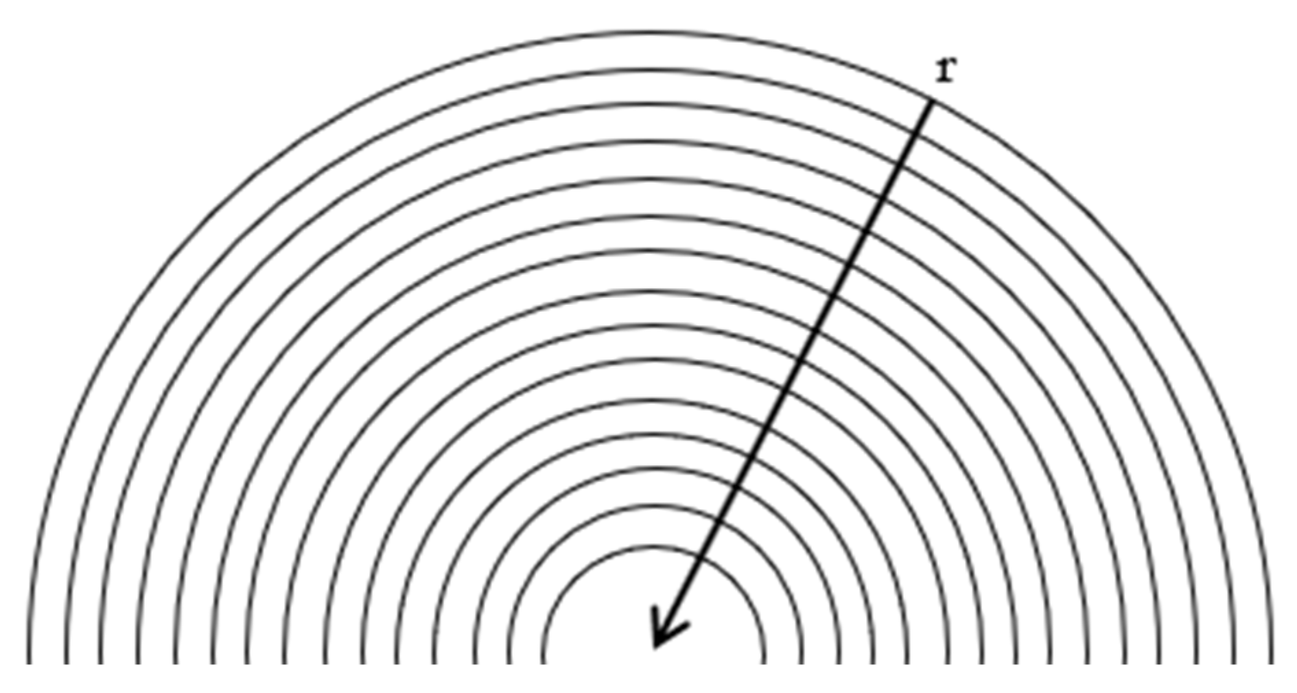
The calculation scheme involves breaking down the spherical droplet into NR concentric shells with uniform thickness, as illustrated in Figure 4. Concentration changes are assessed only radially, simplifying the problem to one dimension. Consequently, the evaluation of Hill’s vortex is omitted. Additionally, the simulation focuses on a droplet of pure fresh water, devoid of alkalis. Hence, reactions (6) and (7) are not considered. Upon analyzing Equations (4) and (5), it was determined that the equilibrium constant of (4) at 25 °C (equal to 1.4 × 10⁻² kmol/m³) significantly surpasses the value of 6.5 × 10⁻⁸ kmol/m³ for (5) at the same temperature. Therefore, the latter is deemed negligible [25]. Under these conditions, only reactions (2.1)–(92.3) are taken into account. However, due to the instability of H₂SO₃, an alternative formulation is utilized by combining reactions (3) and (4):

$$\mathrm{S}{\mathrm{O}}_{2\left(\mathrm{a}\mathrm{q}\right)}+{\mathrm{H}}_2{\mathrm{O}}_{\left(\mathrm{l}\right)}\rightleftharpoons \mathrm{H}\mathrm{S}{\mathrm{O}}_{3\left(\mathrm{a}\mathrm{q}\right)}^{-}+{\mathrm{H}}_{\left(\mathrm{a}\mathrm{q}\right)}^{+}$$

(8)

Equation (8) represents the reaction considered in the absorption model for the interaction between sulfur dioxide and water during the simulation. The chemical mechanism is summarized as follows:

$$\mathrm{S}{\mathrm{O}}_{2\left(\mathrm{g}\right)}\rightleftharpoons \mathrm{S}{\mathrm{O}}_{2\left(\mathrm{a}\mathrm{q}\right)}$$

(8.1)

$$\mathrm{S}{\mathrm{O}}_{2\left(\mathrm{a}\mathrm{q}\right)}+{\mathrm{H}}_2{\mathrm{O}}_{\left(\mathrm{l}\right)}\rightleftharpoons \mathrm{H}\mathrm{S}{\mathrm{O}}_{3\left(\mathrm{a}\mathrm{q}\right)}^{-}+{\mathrm{H}}_{\left(\mathrm{a}\mathrm{q}\right)}^{+}$$

(8.2)

3.2. Droplet Tracking

In a variable droplet system, several considerations are necessary, such as the movement of the particle within the scrubber and the subsequent heat exchange between the droplet and the burned gases, in addition to absorption. These factors have been addressed through a water drop tracking model. The objective of this model is to compute changes in the droplet’s speed, temperature, and diameter over the course of the simulation. The subscripts d and g are used to distinguish quantities related to the droplet and the burned gases, respectively.

3.2.1. Droplet Motion

Inside the scrubbing tower, the droplet is exposed to burned gas moving in the opposite direction. A one-dimensional problem is assumed, with the vertical x-axis parallel to the wash column walls. The origin is set at the outlet of the water spray nozzle, and the positive direction is downwards. Because of the relative motion between the droplet and the gas, it is essential to consider the resistance force that affects the droplet’s motion. This is accounted for using the drag coefficient CD, as described in the following differential Equations [18,24,26]:

$$\frac{\mathrm{d}{\mathrm{u}}_{\mathrm{d}}}{\mathrm{d}\mathrm{t}}=\frac{1}{{\mathsf{\tau }}_{\mathrm{d}}}\left({\mathrm{u}}_{\mathrm{g}}-{\mathrm{u}}_{\mathrm{d}}\right)+\mathrm{a}$$

(9)

$${\mathsf{\tau }}_{\mathrm{d}}=\frac{4 {\mathsf{\rho }}_{\mathrm{d}} {\mathrm{d}}_{\mathrm{d}}^2}{3 {\mathsf{\mu }}_{\mathrm{g}}{\mathrm{C}}_{\mathrm{D}}\mathrm{R}\mathrm{e}}$$

(10)

$$\mathrm{a}=\frac{\mathrm{g}\left({\mathsf{\rho }}_{\mathrm{d}}-{\mathsf{\rho }}_{\mathrm{g}}\right)}{{\mathsf{\rho }}_{\mathrm{d}}}$$

(11)

$$\frac{\mathrm{d}{\mathrm{x}}_{\mathrm{d}}}{\mathrm{d}\mathrm{t}}={\mathrm{u}}_{\mathrm{d}}$$

(12)

where u represents the velocity in m/s, x denotes the position in meters, τ is the characteristic time in seconds, a signifies acceleration in m/s², ρ stands for density in kg/m³, and µ_g represents dynamic viscosity in Pa s. The terms C_D and Re represent the drag coefficient and Reynolds number, respectively. The drag coefficient C_D was computed using the Hadier–Levenspiel equations [27]:

$${\mathrm{C}}_{\mathrm{D}}=\frac{24}{\mathrm{R}\mathrm{e}}\left(1+{\mathrm{b}}_1\mathrm{R}{\mathrm{e}}^{{\mathrm{b}}_2}\right)+\frac{{\mathrm{b}}_3\mathrm{R}\mathrm{e}}{{\mathrm{b}}_4+\mathrm{R}\mathrm{e}}$$

(13)

$${\mathrm{b}}_1=\exp \left(2.3288-6.4581\mathsf{\varphi }+2.4486{\mathsf{\varphi }}^2\right)$$

(14)

$${\mathrm{b}}_2=0.0964+0.5565\mathsf{\varphi }$$

(15)

$${\mathrm{b}}_3=\exp \left(4.905-13.8944\mathsf{\varphi }+18.422{\mathsf{\varphi }}^2-10.2599{\mathsf{\varphi }}^3\right)$$

(16)

$${\mathrm{b}}_4=\exp \left(1.461+12.2584\mathsf{\varphi }-20.7322{\mathsf{\varphi }}^2+15.8855{\mathsf{\varphi }}^3\right)$$

(17)

Φ represents the ratio between the spherical surface area and the surface area of the deformed droplet. Since a spherical droplet is assumed, the constant is equal to unity. As for the Reynolds number, it has been calculated as follows:

$$\mathrm{R}\mathrm{e}=\frac{{\mathsf{\rho }}_{\mathrm{g}}{\mathrm{d}}_{\mathrm{d}}\left|{\mathrm{u}}_{\mathrm{d}}-{\mathrm{u}}_{\mathrm{g}}\right|}{{\mathsf{\mu }}_{\mathrm{g}}}$$

(18)

The solutions to Equations (9) and (5) describe the movement of the droplet inside the scrubbing column at a specific moment t

$${\mathrm{u}}_{\mathrm{d}}^{\mathrm{t}}=\mathrm{w}+\exp \left(-\frac{\Delta \mathrm{t}}{{\mathsf{\tau }}_{\mathrm{d}}}\right)({\mathrm{u}}_{\mathrm{d}}^{\mathrm{t}-1}-\mathrm{w})$$

(19)

$${\mathrm{x}}_{\mathrm{d}}^{\mathrm{t}}={\mathrm{x}}_{\mathrm{d}}^{\mathrm{t}-1}+\Delta \mathrm{t} \mathrm{w}+{\mathsf{\tau }}_{\mathrm{d}}\left(1-\exp \left(-\frac{\Delta \mathrm{t}}{{\mathsf{\tau }}_{\mathrm{d}}}\right)\right)\left({\mathrm{u}}_{\mathrm{d}}^{\mathrm{t}-1}-\mathrm{w}\right)$$

(20)

$$\mathrm{w}={\mathrm{u}}_{\mathrm{g}}+{\mathsf{\tau }}_{\mathrm{d}}·\mathrm{a}$$

(21)

3.2.2. Heat and Mass Exchange between Droplet and Exhaust Gases

The conditions experienced by the droplet during the scrubbing process are variable and directly tied to its own temperature. If the droplet’s temperature is lower than the evaporation temperature, typically around 304 K, there is no exchange of water mass between the droplet and the gas. Instead, there is only a sudden increase in temperature, regulated by the energy balance equation:

$${\mathrm{m}}_{\mathrm{d}}{\mathrm{c}}_{\mathrm{p},\mathrm{w}}\frac{\mathrm{d}{\mathrm{T}}_{\mathrm{d}}}{\mathrm{d}\mathrm{t}}=\mathrm{h}{\mathrm{A}}_{\mathrm{d}}\left({\mathrm{T}}_{\mathrm{g}}-{\mathrm{T}}_{\mathrm{d}}\right)$$

(22)

where m represents the mass in kilograms, c_p,w signifies the specific heat at constant pressure in J/(kg K) of water, h represents the convection coefficient in W/(m²K), and A_d represents the droplet surface area in square meters. To calculate the variation in droplet temperature over time, Equation (22) is solved as follows:

$${\mathrm{T}}_{\mathrm{d}}^{\mathrm{t}}={\mathrm{T}}_{\mathrm{g}}+\left[{\mathrm{T}}_{\mathrm{d}}^{\mathrm{t}-1}-{\mathrm{T}}_{\mathrm{g}}\right]\exp \left(-\mathsf{\alpha }\Delta \mathrm{t}\right)$$

(23)

$$\mathsf{\alpha }=\frac{{\mathrm{A}}_{\mathrm{d}} \mathrm{h}}{{\mathrm{m}}_{\mathrm{d}}{\mathrm{c}}_{\mathrm{p},\mathrm{w}}}$$

(24)

The convection coefficient h was determined using the Ranz–Marshall equation [28]:

$$\mathrm{N}\mathrm{u}=\frac{\mathrm{h}{\mathrm{d}}_{\mathrm{d}}}{{\mathrm{K}}_{\mathrm{g}}}=2.0+0.6\mathrm{R}{\mathrm{e}}_{\mathrm{F}}^{1/2}{\mathrm{P}\mathrm{r}}_{\mathrm{F}}^{1/3}$$

(25)

K_g represents the thermal conductivity of gases in W/(K m), Re_F denotes the Reynolds number, and Pr_F represents the Prandtl number at the film of the droplet.

When the droplet temperatures surpasses the evaporation temperature, mass transfer occurs. The quantification of vaporization is governed by the molar concentration gradient of the vapor between the droplet surface and the exhaust gases:

$${\mathrm{N}}_{\mathrm{w}}={\mathrm{K}}_{\mathrm{w}}({\mathrm{C}}_{\mathrm{w},\mathrm{S}}-{\mathrm{C}}_{\mathrm{w},\mathrm{g}})$$

(26)

where N_w represents the vapor flow between the water drop and gas bulk in kmol/(m²s), K_w denotes the mass transfer coefficient in m/s, and C_w,S and C_w,g represent the molar concentration of vapor at the surface of the droplet and in the exhaust gas, respectively, measured in kmol/m³. The term C_w,S was calculated, assuming that the partial pressure of the vapor at the liquid–gas interface is equal to the saturation pressure (p_sat) at the same temperature:

$${\mathrm{C}}_{\mathrm{w},\mathrm{S}}=\frac{{\mathrm{p}}_{\mathrm{s}\mathrm{a}\mathrm{t}}}{\mathrm{R}{\mathrm{T}}_{\mathrm{d}}}$$

(27)

where R is the universal gas constant equal to 8310 m³ Pa/(kmol K), and p_sat is the saturation pressure in Pa. The concentration of water inside the burned gas was calculated considering the molar fraction x_w,g of water contained therein.

$${\mathrm{C}}_{\mathrm{w},\mathrm{g}}={\mathrm{x}}_{\mathrm{w},\mathrm{g}}\frac{{\mathrm{p}}_{\mathrm{g}}}{\mathrm{R}{\mathrm{T}}_{\mathrm{g}}}$$

(28)

The bulk gas pressure p_g was assumed to be equal to 1 bar. With the molar weight of water known to be 18 kg/kmol, the variation in droplet mass in the scrubbing column over time was obtained from Equation (26):

$${\mathrm{m}}_{\mathrm{d}}^{\mathrm{t}}={\mathrm{m}}_{\mathrm{d}}^{\mathrm{t}-1}-{\mathrm{N}}_{\mathrm{w}} {\mathrm{A}}_{\mathrm{d}} {\mathrm{M}}_{{\mathrm{H}}_2\mathrm{O}} \Delta \mathrm{t}$$

(29)

Hence:

$${\mathrm{d}}^{\mathrm{t}}=2{\left(\frac{3{\mathrm{m}}_{\mathrm{d}}^{\mathrm{t}}}{4\mathsf{\pi }{\mathsf{\rho }}_{\mathrm{d}}}\right)}^{1/3}$$

(30)

Under these conditions, Equation (22) needs to be modified to account for the variation in mass that the drop undergoes due to evaporation:

$${\mathrm{m}}_{\mathrm{d}}{\mathrm{c}}_{\mathrm{p}}\frac{\mathrm{d}{\mathrm{T}}_{\mathrm{d}}}{\mathrm{d}\mathrm{t}}=\mathrm{h}{\mathrm{A}}_{\mathrm{d}}\left({\mathrm{T}}_{\mathrm{g}}-{\mathrm{T}}_{\mathrm{d}}\right)+\frac{{\mathrm{d}\mathrm{m}}_{\mathrm{d}}}{\mathrm{d}\mathrm{t}} {\mathrm{L}}_{\mathrm{g}}$$

(31)

where L_g is the latent heat of the vaporization of water, equal to 23 × 10⁵ J/kg. The solution to Equation (19) is:

$${\mathrm{T}}_{\mathrm{d}}^{\mathrm{t}}=\left({\mathrm{T}}_{\mathrm{p}}^{\mathrm{t}-1}+\mathsf{\beta }\right)\mathrm{e}\mathrm{x}\mathrm{p}(-\mathsf{\gamma }\Delta \mathrm{t})-\mathsf{\beta }$$

(32)

$$\mathsf{\beta }=\frac{{\mathrm{Q}}_{\mathrm{p}}}{{\mathrm{A}}_{\mathrm{d}}\mathrm{h}}-{\mathrm{T}}_{\mathrm{g}}$$

(33)

$$\mathsf{\gamma }=\frac{\mathrm{h}{\mathrm{A}}_{\mathrm{d}}}{{\mathrm{m}}_{\mathrm{d}}^{\mathrm{t}}{\mathrm{c}}_{\mathrm{p},\mathrm{w}}}$$

(34)

$${\mathrm{Q}}_{\mathrm{d}}=\frac{\left({\mathrm{m}}_{\mathrm{d}}^{{\mathrm{t}}_2}-{\mathrm{m}}_{\mathrm{d}}^{{\mathrm{t}}_1}\right)·{\mathrm{L}}_{\mathrm{g}}}{\Delta \mathrm{t}}$$

(35)

When the temperature of the droplet reaches the boiling point T_bp (approximately 373 K at atmospheric pressure), boiling occurs, and the droplet’s temperature remains constant and equal to the boiling point value for the entire duration of this phenomenon. The law governing the reduction in diameter is represented by Equation (30), while the variation in mass is given by:

$${\mathrm{m}}_{\mathrm{d}}^{\mathrm{t}}={\mathrm{m}}_{\mathrm{d}}^{\mathrm{t}-1}-\frac{\mathrm{h}{\mathrm{A}}_{\mathrm{d}}\left({\mathrm{T}}_{\mathrm{g}}-{\mathrm{T}}_{\mathrm{b}\mathrm{p}}\right)\Delta \mathrm{t}}{{\mathrm{L}}_{\mathrm{g}}}$$

(36)

For all cases, the Biot number was calculated as $\mathrm{Bi}=\mathrm{h}·{\mathrm{d}}_{\mathrm{p}}/{\mathrm{k}}_{\mathrm{d}}$, with k_d thermal conductivity of the droplet. This is always higher than 0.1, so the temperature gradient inside the droplet was evaluated using the Fourier equations adapted for a dimension [29]:

$${\mathsf{\rho }}_{\mathrm{d}}{\mathrm{c}}_{\mathrm{d}}\frac{\partial {\mathrm{T}}_{\mathrm{d}}}{\partial \mathrm{t}}={\mathrm{k}}_{\mathrm{d}}\frac{{\partial }^2{\mathrm{T}}_{\mathrm{d}}}{\partial {\mathrm{r}}^2}$$

(37)

with ρ_d and c_d representing the density, specific heat and thermal conductivity of the drop, respectively.

To evaluate the temperature variation along the radius of the drop, Equation (37) was applied to each shell, thus obtaining a discretization of the temperature gradient.

Knowledge of the temperature gradient allows for us to determine the value of chemical parameters (Henry constant and equilibrium) and physical parameters (diffusivity, conductivity, etc.) with greater accuracy, as time and the internal radius vary.

3.3. Absorption Model

The results obtained from the tracking model form the basis for calculations of the amount of SO₂ absorbed by the droplet, as they represent the variations in physical and geometric characteristics.

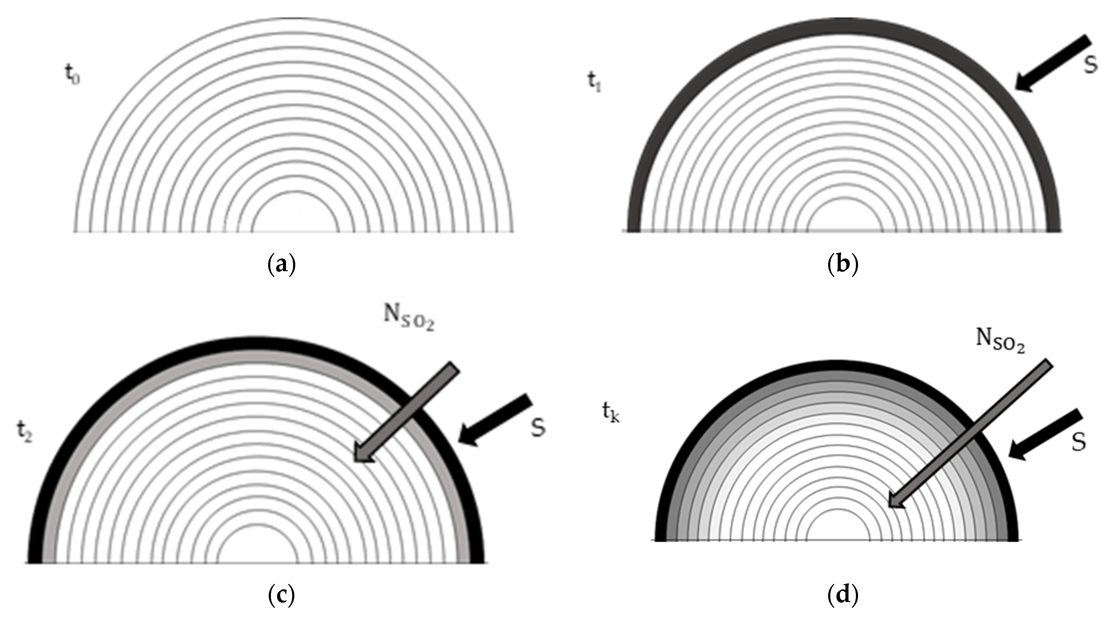
Figure 5 illustrates the first three stages of the model, Figure 5a–c, along with a generic step in Figure 5d. In Figure 5a, the droplet has just entered the scrubbing column and is fully surrounded by the bulk gases. The droplet is still in its initial conditions, as indicated in Table 1. In (b), a flow is established at the interface due to the source term S. Consequently, SO₂ is absorbed as a result of the concentration difference between the droplet and the gas.

In the absence of Hill’s vortex, the saturation of the surface layer occurs instantaneously. However, even under saturation conditions at the surface, the entry of new sulfur dioxide molecules into the droplet continues for two reasons: 1. chemical reaction and 2. diffusive phenomenon.

• Chemical Reaction: When SO₂ enters the droplet, it reacts with water to form ${\mathrm{H}\mathrm{S}\mathrm{O}}_3^{-}$ according to Equation (8). This reaction transforms SO₂, creating space for new molecules. According to Equation (8), the amount of SO₂ concentration that undergoes the reaction is equal to the concentration of ${\mathrm{H}\mathrm{S}\mathrm{O}}_3^{-}$, which can be determined by considering the equilibrium constant of the reaction and its equation [12,16]:

  $${\mathrm{K}}_{\mathrm{a}1}=\frac{{\left[\mathrm{H}\mathrm{S}{\mathrm{O}}_3^{-}\right]}_{\mathrm{e}\mathrm{q}}{\left[{\mathrm{H}}^{+}\right]}_{\mathrm{e}\mathrm{q}}}{{\left[\mathrm{S}{\mathrm{O}}_2\right]}_{\mathrm{e}\mathrm{q}}}=1.9·{10}^{-5}\exp \left[\frac{2022}{\mathrm{T}}\right]\frac{\mathrm{k}\mathrm{m}\mathrm{o}\mathrm{l}}{{\mathrm{m}}^3}$$

  (38)

The concentration of SO₂ at equilibrium is determined by Henry’s law, represented by Equation (1).

2.

The continuous entry of SO₂ into the droplet, despite saturation conditions, is due to the diffusion phenomenon occurring in step (c). In this step, diffusion occurs due to the concentration gradient between the outermost shell and that immediately following. Diffusion acts after the chemical reaction because it is a slower process. The gross rate constant for reaction (3) is approximately 3.4 × 10⁶ s⁻¹ [30,31]. Therefore, it has been assumed that the chemical reaction and the new entry are instantaneous, ensuring continuous saturation conditions at the external volume.

3.

In Figure 5d, the droplet’s condition at a generic kth instant is represented. SO₂ continues to diffuse inward, and droplet evaporation is ongoing, resulting in a reduction in volume.

4.

To calculate the variation in sulfur dioxide concentration over time, the species equation can be utilized [17]:

$$\frac{\partial \mathrm{C}}{\partial \mathrm{t}}=-\nabla ·\left(\mathrm{C}·\mathbf{u}\right)-\mathrm{D}{\nabla }^2\mathrm{C}+\mathrm{S}$$

(39)

5.

where C represents the concentration of SO₂ in kmol/m³, t is the time in seconds, u is the velocity vector of sulfur dioxide molecules inside the droplet in m/s, D is the diffusion coefficient of SO₂ in m²/s, and S is the source term in kmol/m³s in the examined case. ∇⋅(Cu) represents the convective term, and D∇²C represents the diffusive term.

Given the one-dimensional nature of the problem, Equation (39) can be expressed as follows:

$$\frac{\partial {\mathrm{C}}_{\mathrm{i}}}{\partial \mathrm{t}}=-{\mathrm{D}}_{\mathrm{i}}{\nabla }^2{\mathrm{C}}_{\mathrm{i}}+\mathrm{S}$$

(40)

The diffusive term in Equations (39) and (40) represents Fick’s second law, which describes non-stationary motion [32]. The negative sign signifies the direction of movement from the highest to the lowest concentration. In the following sections, both the source and diffusive terms will be presented analytically.

3.3.1. Source Term

The source term determines the flow of matter between the bulk gas and the droplet; therefore, it acts only on the surface volume. In this case, the flow takes place between two different states; therefore, different mass transfer coefficients should be considered compared to the previous case. Additionally, the lack of a Hill vortex suggests a very quick saturation of the surface volume, reducing absorption.

Assuming that the chemical reaction takes place faster than diffusion, not all SO₂ diffuse instantaneously inside the drop, but only a small part obtained from the difference between reactants and products of the (3). The equilibrium concentration of the $\mathrm{H}\mathrm{S}{\mathrm{O}}_3^{-}$ can be obtained from (38). The concentration in an aqueous solution of sulphur dioxide, in saturation conditions, is regulated by (1). The Henry constant k_H can be expressed by [12,16]:

$${\mathrm{k}}_{\mathrm{H}}=7.1·{10}^{-4} {\mathrm{e}}^{\frac{3145}{\mathrm{T}}}/\mathrm{R}\mathrm{T} \frac{\mathrm{m}\mathrm{o}\mathrm{l}}{\mathrm{L}}\mathrm{a}\mathrm{t}\mathrm{m}$$

(41)

The concentration of ${\mathrm{H}\mathrm{S}\mathrm{O}}_3^{-}$ at equilibrium represents the quantity of SO₂ that reacts in Equation (8). Consequently, only the remaining portion diffuses inside the droplet. Assuming that saturation concentration at the surface volume is reached at the initial instant, it is presumed that the droplet can absorb the quantity of SO₂ that reacted in the previous instant. Therefore, a constant saturation occurs on the surface volume. The flow of sulfur dioxide entering at time t is given by:

$${\mathrm{S}}_t={\left[\mathrm{H}\mathrm{S}{\mathrm{O}}_3^{-}\right]}_{1,\mathrm{t}}\frac{{\mathrm{V}}_{1,\mathrm{t}}}{{\mathrm{A}}_{1,\mathrm{t}}}\frac{1}{\Delta \mathrm{t}}$$

(42)

3.3.2. Diffusive Term

The diffusive term represents the flow of SO₂ within the droplet, from the external to the internal layers. To further simplify the model, an alternative formulation is used instead of Equation (39) [9]:

$${\mathrm{N}}_{\mathrm{S}{\mathrm{O}}_2}={\mathrm{K}}_{\mathrm{l}}({\mathrm{C}}_{\mathrm{b}}-{\mathrm{C}}_{\mathrm{a}})$$

(43)

The molar flow of sulfur dioxide (N_SO2) occurs between two adjacent volumes and is measured in kmol/m²s. C_b represents the concentration term of volume i − 1 concerning the volume ith under examination at the same instant. Similarly, C_a represents the concentration at volume i, following volume i − 1 towards the center of the droplet. K_l denotes the local mass transfer coefficient of SO₂ in water, measured in m/s.

The influx and efflux of matter in this volume (28.1 and 28.2) were evaluated through a mass balance conducted in volume i. This analysis was performed for volumes i, i = 1, ..., NR, progressing towards the inner layers of the droplet.

$${\mathrm{N}}_{\mathrm{i}-1,\mathrm{i}}^{\left(\mathrm{t}\right)}={\mathrm{K}}_{\mathrm{l}}\left({\mathrm{C}}_{\mathrm{i}-1}^{\left(\mathrm{t}-1\right)}-{\mathrm{C}}_{\mathrm{i}}^{\left(\mathrm{t}-1\right)}\right)$$

(44)

$${\mathrm{N}}_{\mathrm{i},\mathrm{i}+1}^{\left(\mathrm{t}\right)}={\mathrm{K}}_{\mathrm{l}}\left({\mathrm{C}}_{\mathrm{i}}^{\left(\mathrm{t}-1\right)}-{\mathrm{C}}_{\mathrm{i}+1}^{\left(\mathrm{t}-1\right)}\right)$$

(45)

The quantity of matter remaining in i within the time ∆t interval:

$${\mathrm{M}}_{\mathrm{i}}^{\left(\mathrm{t}\right)}={\mathrm{N}}_{\mathrm{i}-1,\mathrm{i}}^{\left(\mathrm{t}\right)}-{\mathrm{N}}_{\mathrm{i},\mathrm{i}+1}^{\left(\mathrm{t}\right)}={\mathrm{K}}_{\mathrm{l}}\left({\mathrm{C}}_{\mathrm{i}-1}^{\left(\mathrm{t}-1\right)}-{\mathrm{C}}_{\mathrm{i}+1}^{\left(\mathrm{t}-1\right)}\right)$$

(46)

The concentration in i is represented as follows:

$${\mathrm{C}}_{\mathrm{i}}^{\left(\mathrm{t}\right)}={\mathrm{M}}_{\mathrm{i}}^{\left(\mathrm{t}\right)}·\frac{{\mathrm{A}}_{\mathrm{i},\mathrm{t}}}{{\mathrm{V}}_{\mathrm{i},\mathrm{t}}}\Delta \mathrm{t}+{\mathrm{C}}_{\mathrm{i}}^{(\mathrm{t}-1)}$$

(47)

Considering A_i,t as the surface area through which the incoming and outgoing flows pass at the instant t, and given that the thickness of the shell is negligible, an approximation was made by assuming that, for the same volume, V_i,t, the inlet and outlet surfaces have the same size at the same instant.

Additionally, reaction (8) also occurs within the internal volumes of the drop. Therefore, the volumes were adjusted by subtracting an amount of [${\mathrm{H}\mathrm{S}\mathrm{O}}_3^{-}$]_i,t when evaluating the diffusive flux. Equation (46) has been modified accordingly:

$${\mathrm{M}}_{\mathrm{i}}^{\left(\mathrm{t}\right)}={\mathrm{K}}_{\mathrm{l}}\left({\mathrm{C}}_{\mathrm{i}-1}^{\left(\mathrm{t}-1\right)}-{\left[\mathrm{H}\mathrm{S}{\mathrm{O}}_3^{-}\right]}_{\mathrm{i}-1}^{\left(\mathrm{t}-1\right)}-{\mathrm{C}}_{\mathrm{i}-1}^{\left(\mathrm{t}-1\right)}\right)$$

(48)

4. Results

The simulations for both droplet tracking and absorption models were conducted by varying the initial values of drop diameter, flue gas temperature, and SO₂ concentration within the intervals specified in Table 1.

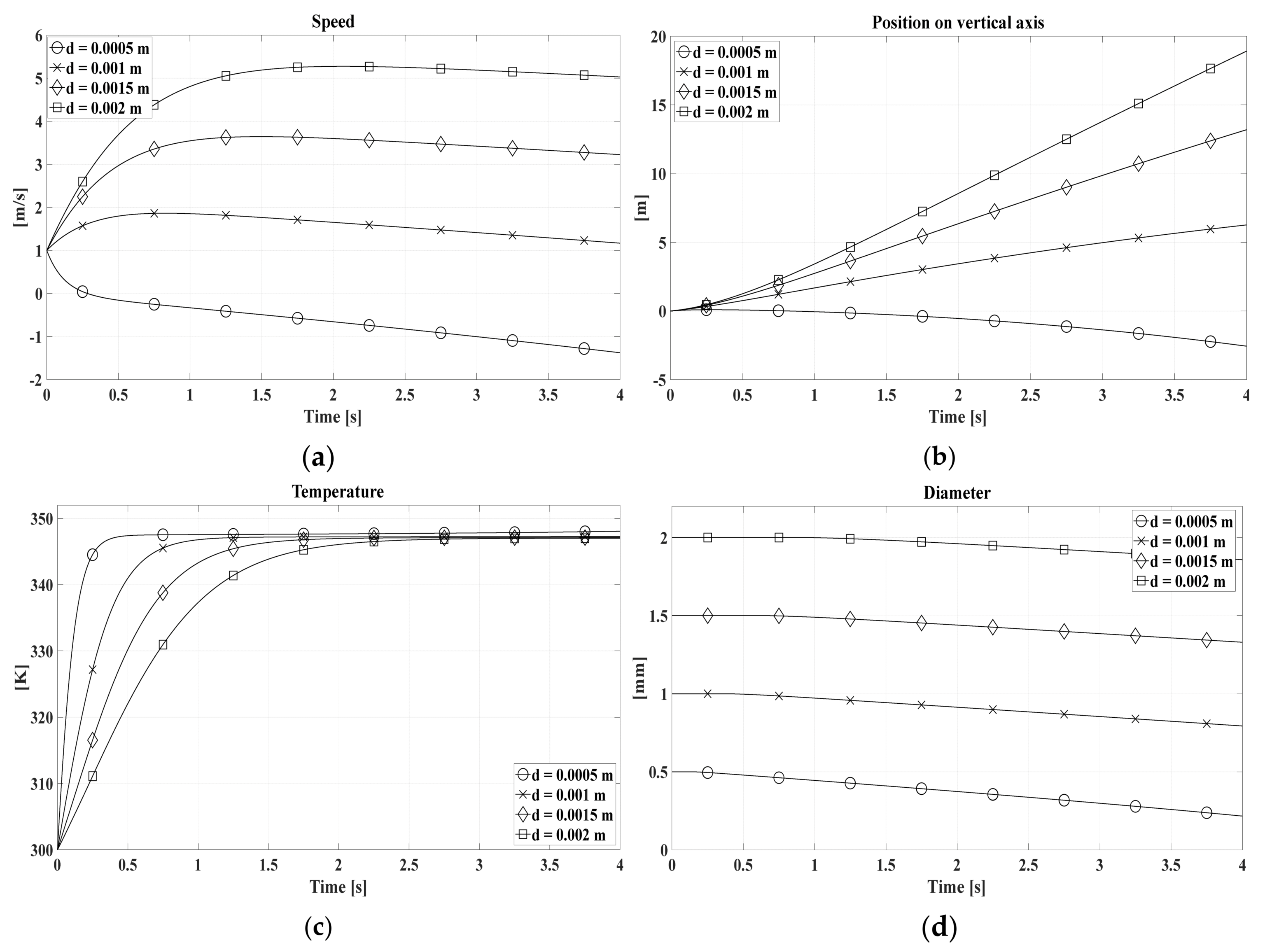
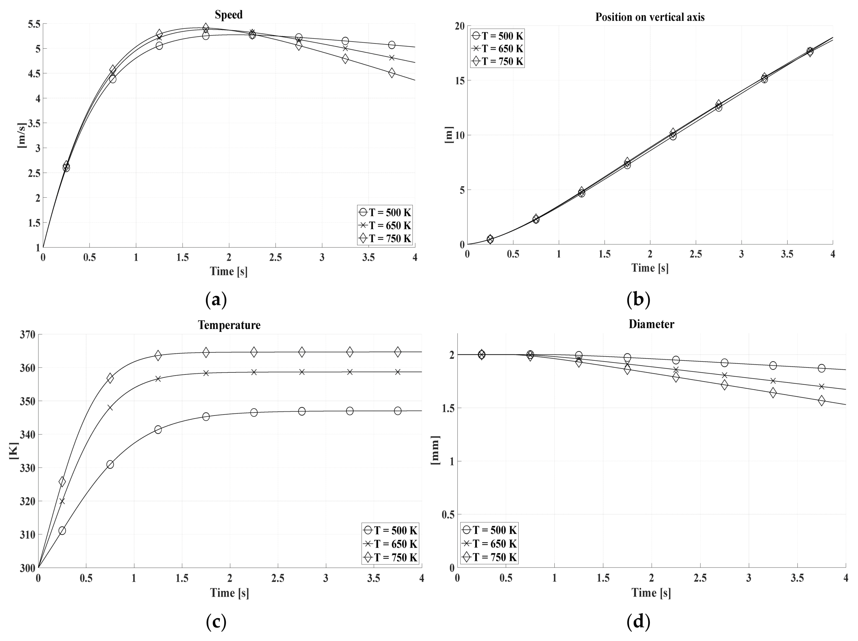
In the droplet tracking model, the evaluation involved four variables: (a) velocity, (b) position, (c) temperature, and (d) diameter. A time step (Δt) of 0.0005 s was used for a simulation duration of 4 s.

The analysis revealed that the different concentrations of sulfur dioxide that were examined did not significantly affect the model. Consequently, only the results related to a concentration of 620 ppm were reported. Figure 6 illustrates the behavior of droplet properties for various diameters at a combustion gas temperature of 500 K. It is noteworthy that droplets with a diameter of 0.5 mm are swiftly carried away by the gaseous stream and evaporate rapidly. Consequently, 0.5 mm droplets are unsuitable for this purpose.

In Figure 7 and Figure 8, kinematic and thermodynamic properties of droplets were analyzed for different bulk gas temperatures, considering diameters of 1 mm and 2 mm, respectively. At a bulk gas temperature of 750 K, thermal equilibrium between water and gas occurs at higher temperatures, leading to rapid volume and mass reduction according to Equations (22) and (19). As a result of this mass decrease, the 1 mm droplet changes its trajectory at 3.021 s within the scrubbing tower, being carried by the bulk gas toward the atmosphere (Figure 7b). Consequently, at 750 K, a 1 mm droplet should not remain in the scrubbing column for more than 3.0 s, necessitating a tower height shorter than 3.34 m (Figure 7d).

Regarding the 2 mm diameter droplet illustrated in Figure 8, the impact of increasing flue gas temperatures is not as significant as that observed with the 1 mm droplet. Although temperature variations are observed across different flue gas temperatures, as depicted in Figure 8c, thermal equilibrium is reached at a slower rate compared to the previous case. Consequently, these variations do not result in substantial consequences, such as trajectory alterations, within the simulation time for the 2 mm droplet (Figure 8b).

In the absorption model, the analysis was conducted using a time step of 0.0004 s for a total duration of 3.2 s, resulting in 8000 iterations for each case study. The droplets were divided into 50 concentric shells, excluding the 0.5 mm droplet, for which results were not reported.

Figure 9 depicts the ratio between the average concentration and saturation concentration over time under various boundary conditions, including varying sulfur dioxide concentration in bulk gases (Cg) and different gas temperatures (Tg). This trend closely aligns with the behavior of saturation concentration, as described by Henry’s law and, consequently, Henry’s constant, as expressed in Equation (41).

Initially, the average concentration (Cm) of smaller drops increases at a faster rate. However, this trend shifts due to the higher temperature, resulting in a lower saturation concentration (Cs). Additionally, the reduction in volume also affects the phenomenon, leading to a subsequent increase in average SO₂ concentration.

An elevation in bulk gas temperature causes a decrease in absorbed SO₂ without significant changes in the trend, as depicted in Figure 9a,b. Similarly, a higher sulfur dioxide concentration notably impacts the trend, as shown in Figure 9a–c, although the saturation condition is significantly distant. At 920 ppm, the influence of exhaust gas temperature becomes more prominent than that at 620 ppm (Figure 9c,d).

The inlet sulfur dioxide concentration within the droplets was also assessed (Figure 10). The results indicate that a 2 mm droplet is capable of absorbing more sulfur dioxide than a smaller droplet. The boundary conditions play a significant role in this trend: at a temperature of 750 K, the amount of absorbed SO₂ is lower compared to 500 K due to droplet evaporation and the decreasing trend of saturation concentration (Figure 10a,b), (Figure 10c,d).

When the sulfur dioxide concentration (C_g) is 620 ppm and the temperature of the bulk gases (T_g) is 500 K (Figure 10a), droplets with diameters of 1 mm, 1.5 mm, and 2 mm absorb 2.60 × 10⁻⁶ g, 1.08 × 10⁻⁵ g, and 2.97 × 10⁻⁵ g of SO₂, respectively. At the same sulfur dioxide concentration and a bulk gas temperature of 750 K (Figure 10b), the absorbed amounts of SO₂ decrease to 1.09 × 10⁻⁶ g for a 1 mm droplet, 5.44 × 10⁻⁶ g for a 1.5 mm droplet, and 1.62 × 10⁻⁵ g for a 2 mm droplet.

The variation in sulfur content in the bulk gas also influences this phenomenon. As the amount of sulfur dioxide in the exhaust gases increases, the saturation concentration also rises, allowing more SO₂ to be absorbed by the droplets (Figure 10a–c), (Figure 10b–d). In Figure 10c, the mass of absorbed SO₂ reaches 3.81 × 10⁻⁶ g for a 1 mm droplet, 1.59 × 10⁻⁵ g for a 2 mm droplet, and finally 4.36 × 10⁻⁵ g for a 2 mm droplet. Despite the high concentration of SO₂ in the bulk gases, at temperatures up to 750 K, the amount of inlet SO₂ mass is lower compared to 500 K (Figure 10d). In this scenario, the absorbed masses are 1.60 × 10⁻⁶ g for a 1 mm droplet, 7.99 × 10⁻⁶ g for a 1.5 mm droplet, and 2.37 × 10⁻⁵ g for a 2 mm droplet.

The absorption capacity of a specific mass of water for SO₂ was further investigated, as depicted in Figure 11. This specified mass was considered equivalent to that of a droplet with a 2 mm diameter. The count (N_i) of droplets ranging from 1 mm to 1.5 mm that could combine to form a mass equivalent to that of a 2 mm droplet was determined. It was observed that a 2 mm droplet possesses a mass 8 times greater than that of a 1 mm droplet (N_1.0 = 8) and 2.3704 times greater than that of a 1.5 mm droplet (N_1.5 = 2.3704).

Figure 11 illustrates that smaller droplets with a diameter of 1 mm (N_1.0) exhibit a higher capacity to absorb sulfur dioxide compared to larger droplets due to their superior surface-to-volume ratio. Specifically, under typical conditions of SO₂ concentration and temperature (620 ppm and 500 K, respectively, common values for naval bulk gases), 1 mm droplets can absorb approximately 1.8 × 10⁻⁴ g, whereas 2 mm droplets absorb only about 2.9 × 10⁻⁵ g.

5. Conclusions

In this study, we developed a simplified numerical model to simulate the absorption of sulfur dioxide (SO₂) by water droplets within a scrubbing column, immersed in the exhaust gases of a naval diesel engine. The model, although simplified, offers valuable insights into the SO₂ absorption process. Our findings provide essential considerations for optimizing wet scrubber efficiency and determining the minimum droplet size necessary for effective SO₂ capture.

The simulations, conducted under diverse Initial conditions outlined In Table 1, revealed important observations. Firstly, the 0.5 mm droplet, identified as the smallest, proved impractical due to its swift displacement by the flow. Consequently, it was excluded from further consideration in the absorption model. Across all scenarios, saturation within the entire droplet was not achieved due to the absence of a convection term. Instead, saturation occurred only in the outermost layers, leading to a slower absorption process. This effect was exacerbated by the droplet volume reduction due to evaporation, resulting in elevated average concentrations, especially in the outer layers. As a consequence, a smaller amount of SO₂ penetrated the droplet. Consequently, for a single droplet, the 2 mm diameter droplet demonstrated a superior SO₂ absorption capacity.

We observed a high sensitivity of SO₂ absorption to increases in SO₂ concentration in the exhaust gas. For the 2 mm droplet at 500 K, absorption reached 4.36 × 10⁻⁵ g, decreasing to 2.37 × 10⁻⁵ g at 750 K for the combustion gases. However, when considering the overall number of droplets required to achieve a specific mass, we found that a group of N_1.0 1 mm droplets was more efficient in absorption due to their higher surface-to-volume ratio. In this context, the simulation indicated an absorption of 1.8 × 10⁻⁴ g of SO₂, surpassing the value achieved with 2 mm droplets by a factor of 5.77.

In summary, our study not only sheds light on the intricate dynamics of SO₂ absorption by water droplets in practical scrubbing scenarios but also underscores the importance of droplet size and concentration in optimizing absorption efficiency in wet scrubber systems. These insights provide valuable guidance for designing more effective and efficient pollution-control methods in industrial and naval settings.

The data put in evidence that there is a strong correlation between the environment concentration and the mass flow rate incoming inside the droplets. The mass flow rate analysed for the indicated boundary conditions are comparable with what is found in the literature [25]. Furthermore, the equations are developed explicitly, meaning that the reaction (8) is considered in the mass balance, along with its equilibrium constant. The method described in this study takes into account the diffusivity and equilibrium constants of reactions (2) and (8) that often are resumed in one parameter β [33], leading to quite similar results, with a maximum deviation of 30%. This leads us to consider that the methods that are used, although approximate, as defined in a one-dimensional field, provides results comparable to those in the literature.