
The Elusive Nature of “Seeing”


Cerro Tololo Inter-American Observatory|NSF’s NOIRLab, Casilla 603, La Serena 1720236, Chile
Atmosphere 2023, 14(11), 1694; https://doi.org/10.3390/atmos14111694
Submission received: 9 September 2023
/
Revised: 11 October 2023
/
Accepted: 19 October 2023
/
Published: 17 November 2023
(This article belongs to the Special Issue The Impacts of Climate on Astronomical Observations)
Abstract
:Atmospheric image blur, “seeing”, is one of the key parameters that influences the selection of observatory sites and the performance of ground-based telescopes. In this review, the common definition of seeing based on the Kolmogorov turbulence model is recalled. The ability of this model to represent real, non-stationary fluctuations of the air refractive index is discussed. Even in principle, seeing (a model parameter) cannot be measured with arbitrary accuracy; consequently, describing atmospheric blur by a single number, seeing, is a crude approximation. The operating principles of current seeing monitors are outlined. They measure optical effects caused by turbulence, sampling certain regions of spatial and temporal spectrum of atmosphreic optical disturbances, and interpret their statistics in the framework of the standard model. Biases of seeing monitors (measurement noise, propagation, finite exposure time, optical defects, wind shake, etc.) should be quantified and corrected using simulations, while instrument comparison campaigns serve as a check. The elusive nature of seeing follows from its uniqueness (a given measurement cannot be repeated or checked later), its non-stationarity (dependence on time, location, and viewing direction), a substantial role of the highly variable surface layer, and a potential bias caused by the air flow in the immediate vicinity of the seeing monitors. The results of seeing measurements are outside the scope of this review.
1. Introduction
The term seeing is universally accepted to describe the image blur in ground-based telescopes caused by optically inhomogeneous air; the latter is often called turbulence or, more precisely, optical turbulence. The random motion of air associated with turbulence is, by itself, not harmful to the observations; it produces seeing only when air packets of different temperatures are mixed, creating spatial variations in the refractive index. The propagation of light through the optically inhomogeneous atmosphere is the cause of seeing [1]. The review by Coulman [2] is an excellent introduction to the subject with an emphasis on the physics of turbulence.
Astronomers used to evaluate atmospheric blur qualitatively and approximately, until linear light detectors replaced the eye and the photographic plate. The blur is quantified by the point spread function (PSF), which is nothing else but an image of a point source (star). The Full Width at Half Maximum (FWHM) of the PSF is a quantitative measure of seeing. However, the PSF is usually enlarged by other factors (e.g., optical imperfections of the telescope, guiding errors, atmospheric dispersion, etc.). If all individual blur factors can be approximated by Gaussian functions with dispersions , the resulting dispersion is . The FWHM of a Gaussian is 2.35. The PSF can be measured quite accurately. When reliable estimates of other blurring factors are available, the dispersion corresponding to the atmospheric blur can deduced by quadratic subtraction of these factors, leading to the value of seeing, . Seeing is measured in angular units—arcseconds or radians.
In reality, the PSF of the atmospheric blur is not exactly Gaussian. Other contributors to the PSF are usually poorly known and the PSF itself is not rotationally symmetric. Using the above simplistic approach with biased estimates of the “instrumental” blur factors can lead to biased (often too optimistic) estimates of the seeing at a given observatory. For example, Racine et al. [3] estimated the median “natural” seeing at the Mauna Kea observatory at 0.43 using this approach, while 0.75 was actually measured later [4].
The utility of measuring seeing quantitatively and independently of the telescope is clear. Such measurements are particularly needed for the exploration of new astronomical sites. The critical role of seeing as a fundamental limitation of ground-based astronomy has been fully recognized in the middle of the 20th century [5]. This has led to a search of new sites with better seeing and to the construction of new major observatories at these sites–in Arizona, Chile, on Canary islands, and on Mauna Kea. The idea of placing telescopes in space has crystallized at the same time, and the success of the Hubble Space Telescope with its modest 2.4 m aperture and diffraction-limited PSF is an excellent illustration of the key role of seeing.
Methods of measuring atmospheric seeing with relatively small instruments and their limitations is the main subject of this review (Section 3); the definition of seeing, covered in Section 2, is based on the theory of optical propagation that also appeared in the middle of the 20th century [6]. Initially, though, astronomers were not aware of this theory and developed their first seeing monitors based on heuristic approaches. They measured atmospheric image wobble in a small telescope [7,8] or a differential image motion in two small telescopes separated by ∼3 m [9]. Traditional light detectors (eye and photographic plate) did not produce quantitative data, and first-generation seeing monitors were usually “calibrated” against image blur in nearby large telescopes.
The development of the atmospheric theory, modern light detectors, and new techniques such as adaptive optics (AO), driven originally by military applications rather than by astronomy, eventually gave birth to the modern generation of quantitative seeing monitors in the 1970s [10,11]. All seeing monitors are based on the standard model of atmospheric perturbations, often called the Kolmogorov-Obukhov model. The underlying concept is a random stationary process, implying isotropic and statistically homoheneous perturbations that do not change their statistics with time. The real atmosphere is anything but stationary; the motion of the air is chaotic and fundamentally unpredictable. The standard atmospheric theory is a good match to reality in some, but not all, applications. The definition of atmospheric seeing (Section 2) is anchored to the standard model and looses its meaning otherwise. This fact is often overlooked, and seeing is perceived as a well-defined parameter that can be measured with almost arbitrary accuracy, similar to other meteorological parameters like temperature or wind speed. The elusive character of seeing is covered in Section 4. The last Section 5 summarizes the material and outlines current trends in development and the use of seeing monitors. The results of seeing campaigns, seeing statistics at various sites, global trends, etc. comprise a vast subject which remains outside the scope of this review; only the definitions and methods are covered here. As this topic is quite mature, many old classical papers are cited. Meanwhile, seeing measurements are being actively pursued in different parts of the world (e.g., [12,13,14]), and new methods are being developed.
2. Definition of Seeing and
The standard theory of light propagation through the atmosphere is covered in a number of textbooks and reviews, for example [6,15,16,17]. Its main points relevant for seeing are summarized here briefly. The theory assumes that refractive-index fluctuations in the air correspond to a random stationary process with a particular form of the power spectrum (the Kolmogorov-Obukhov model). It is postulated that mechanical energy of turbulent air motion is injected at a constant rate at some large spatial scale (the outer scale), then it is transferred to progressively smaller eddies in a cascade, and eventually dissipates by viscosity at the smallest inner scale , on the order of a few mm. The structure function (SF) of the air refractive index in the intermediate (inertial) range between and has a particular power-law form derived from dimensional considerations:
where the coefficient , called refractive index structure constant, determines the strength of the fluctuations. Turbulence is assumed to be isotropic, so the SF depends only on the modulus of the distance between two points in space, . Angular brackets denote averaging over statistical ensemble. The definition of the parameter , measured in , is tied to Equation (1). An extension of the theory to a power law that differs from 2/3 has been proposed, but it has not become popular; the extension loses its physical grounds (the turbulent cascade) and becomes a purely mathematical exercise.
The universally adopted definition of seeing is deduced from the above postulate in several steps outlined below. The seeing depends on the total power of turbulence along the line of sight, called turbulence integral , where z is the propagation distance. The integral is measured in .
Phase of the light wave that passed through a turbulent layer is also a random stationary process with a power spectrum
The phase perturbations are isotropic, and their spectrum depends only on the modulus of the two-dimensional spatial frequency ; the frequency is measured in . The light wavelength is . The corresponding phase structure function of a perturbed wave-front is
where r is the distance between two points on the wave-front, . The parameter (Fried’s radius) is related to the turbulence integral J. It is a distance where the atmospheric rms phase difference reaches radians [18]:
The power-law phase SF implies an infinite phase dispersion, but (3) is valid only at , in the inertial range. The additional parameter (outer scale) can be introduced explicitly into Equations (2) and (3) in several ways, of which the von Kàrmàn formula is the most popular option. In many typical applications of the theory the effect of the finite outer scale can be neglected, at least to the first order.
Atmospheric phase distortions at the telescope pupil result from the sum of all turbulent layers, and it is safe to assume that the random phase perturbations are normally distributed, even if the underlying refractive-index fluctuations are not Gaussian. Then the atmospheric optical transfer function (Fourier transform of the PSF in a long-exposure image in a large-aperture telescope) is related directly to the phase SF:
The PSF depends on the angular coordinates (in radians), and are corresponding spatial frequencies (in , ). The PSF is normalized to a unit integral, hence .
The Equation (5) explains why the inner and outer scales of turbulence play only a minor role in the image blur caused by seeing. At small scales the SF is , so always. Similarly, at we have , , and the exact behavior of is irrelevant. At optical wavelengths, m is in the middle of the inertial range. However, it is larger in the infra-red (recall that ), where the effects of the outer scale (on the order of 20 m) become more relevant. With a finite outer scale, grows slower than , the OTF becomes larger, and the resolution improves.
The 5/3 power index in (5) is close to 6/3 = 2 that corresponds to a Gaussian law, therefore the atmospheric OTF is approximately Gaussian, and its Fourier transform, the PSF, also resembles a Gaussian (it has a slightly sharper core and stronger wings). The parameter was defined by Fried [18] so that the integral of the atmospheric OTF equals . Thus, the seeing-limited resolution, expressed by this integral, equals the diffraction-limited resolution of a perfect telescope with aperture diameter . The FWHM of the atmospheric PSF equals
and this equation is the formal definition of the seeing. The parameters , , and J express the same quantity in different ways and in different units (radians, meters, and , respectively), but they are equivalent. Table 1 gives conversions from one to another.
Strictly speaking, (6) is valid only for infinite outer scale; with a finite , the resolution improves, and an approximate formula can account for this effect, as long as it remains minor [19]. Floyd et al. [20] demonstrated that PSF in a well-tuned telescope is indeed sharper than predicted by the site monitor; unlike Racine et al. [3], they made no assumptions about imperfect optics, dome seeing, etc. Although the atmospheric blur depends, strictly speaking, on two parameters , the standard definition of seeing ignores for a good reason—simplicity.
The standard theory neglects dispersion of the air and assumes that fluctuations of the wave-front are achromatic; the turbulence integral J does not depend on the imaging wavelength . However, the phase of light waves scales as , which leads to and . When the seeing is characterized by parameters or , it is mandatory to specify also the wavelength (e.g., 500 nm). In astronomical observations at some zenith distance , the turbulence integral is proportional to , so the seeing depends on the zenith distance as . Seeing measurements are usually corrected to (zenith) using this scaling.
To summarize, seeing is defined as a single parameter of the random stationary process with a 5/3 power spectrum. Seeing can be equivalently expressed by the parameters J, , or , but the last two depend also on the wavelength. How well this standard theory matches the real atmosphere is an open question, partly discussed below. In theory, turbulence is stationary and isotropic, hence does not depend on position and time. In reality, turbulence along the line of sight is not uniform, and we often measure the turbulence profile . Turbulence also evolves with time, violating the assumed stationarity.
The statistical theory operates with ensemble averaging, although in reality there is only one realization of the random process (atmospheric turbulence). This common caveat is circumvented by assuming ergodicity and replacing the ensemble average by averaging over time. In fact, the process is not stationary, and the longer we average, the more likely are variations in the measured quantity. Thus, from the outset we have to admit that such parameters as or seeing are only approximate estimates that cannot be measured or even defined with arbitrary accuracy. This problem is particularly severe for the outer scale , where we deal effectively with only one “cycle” (a large-scale disturbance decaying into a small-scale cascade). The concept of power spectrum becomes almost meaningless when applied to large-scale and non-stationary perturbations, so attempts to measure this spectrum are futile. The best approach is to assume a particular form of the power spectrum at low frequencies and to deduce by comparing theoretical predictions derived from the assumed spectrum with observed effects. In this sense, is even more elusive than the seeing.
Seeing is an elusive quantity for yet another reason: each its measurement is unique, it cannot be repeated or verified because conditions always evolve. Of course, two seeing monitors located closely to each other and looking at the same star can be inter-compared reliably. If a systematic difference between them is revealed, it can be modeled and accounted for. However, it is not known a priori which instrument gives less biased results. Furthermore, the difference between instruments depends on the conditions, so calibrating seeing monitors against some “standard” instrument does not guarantee reproducible and reliable results (e.g., for comparing astronomical sites). Nowadays, computers allow comprehensive simulation of turbulence, propagation through the atmosphere, and the instrument itself. Using simulations, we can evaluate the instrumental biases because the true (simulated) seeing is always known. So, the correct method of calibrating seeing monitors and accounting for their biases is by “measuring” simulated turbulence that, naturally, conforms to the standard theory.
3. Optical Methods of Seeing Measurement
Fluctuations of the air refractive index are caused mostly by fluctuations of air temperature which can be measured by fast in situ sensors [21]. The techniques used for such micro-thermal measurements are not considered here. We focus instead on the optical methods where distortions of the light waves caused by turbulence are measured and interpreted in terms of seeing. Optical methods of turbulence sounding have the advantage of being direct (no conversion from temperature to refractive index) and non-invasive. They usually sample the full propagation path and are relatively inexpensive, allowing continuous monitoring of observing conditions. In this review, a detailed description of the operational principles and construction of seeing monitors is skipped (it can be retrieved from the cited literature); instead, the relation of measured quantities to seeing and unavoidable instrumental biases are highlighted.
In adaptive optics (AO) [22,23,24], wave-fronts are measured with a certain spatial and temporal resolution, and the seeing can be deduced from these data. The wave-front phase distortions can be represented by a combination of some base functions (modes), such as Zernike polynomials of increasing order: tilts, defocus, astigmatisms, etc. The theory tells us that atmospheric variance of each mode is proportional to with coefficients that decrease with increasing mode order [25]; this is a consequence of the turbulence spectrum where low spatial frequencies always dominate. So, to obtain a larger signal from atmospheric distortions, we have to use the lowest-order modes and/or to increase the telescope diameter D. For practical reasons (portability and cost), small apertures are preferable, so most seeing monitors measure tilts and curvature (defocus) because these effects are the largest.
Propagation through turbulent atmosphere distorts both phase and amplitude of the light waves. Amplitude distortions imply fluctuations of the light flux, scintillation. Scintillation becomes important at spatial scales comparable to and smaller than the Fresnel radius , where z is the propagation distance ( m for km and nm). In AO, scintillation is usually neglected, but it can serve for measuring seeing: seeing monitors can use phase distortions, scintillation, or both. The strongest turbulence is usually located at low altitudes and produces negligible scintillation, so seeing monitors based on phase distortions are more popular than those based on scintillation.
3.1. Coherence Interferometers
Optical propagation converts part of phase fluctuations into amplitude fluctuations. However, the formula for the optical transfer function (5) remains invariant to propagation if the phase SF is replaced by the sum of phase and amplitude SFs, . The atmospheric OTF in fact is the coherence function (CF) of distorted light at a distance . This CF can be measured by organizing interference at a baseline (shift) r and recording the contrast of the resulting fringes averaged over time. An interferometer where wave-front interferes with its inverted or rotated copy allows us to measure the atmospheric CF over a range of baselines by taking a single long-exposure image of the fringes. Dependence of the fringe contrast on the baseline r gives a direct measurement of by fitting the theoretical formula .
This elegant and theoretically perfect method of measuring the seeing was proposed in the 1970s by two groups. In the instrument constructed by Dainty and Scaddan [11], the wave-front was rotated by 180 and combined with the original non-rotated wave-front. The coherence interferometer constructed by Roddier and Roddier [26] implemented rotation by an arbitrary angle, allowing them to use larger apertures and, hence, to gather more light. In theory, optical turbulence is isotropic and it is sufficient to measure the CF in only one direction by combining the wave-front with its mirror-inverted copy [27]. The contrast of fringes for a reflected or rotated wave-fronts is sensitive to polarization, and half of the light is usually lost in the polarizer. Such interferometers are delicate devices involving beam-splitters, mirrors, and precise mechanics. A simplified version of the compact and robust coherence interferometer where the light interferes via grazing reflection from a mirror (the Lloyd mirror) and there is no need for a polarizer is more practical [28].
Coherence interferometers are not used widely as seeing monitors for a trivial but important reason: the wave-front distortions in real telescopes are produced not only by the atmosphere. The impact of static aberrations is not relevant (they distort the fringes statically but do not affect their contrast in a long exposure), but random tilts caused by wind shake of the telescope or by imperfect tracking is a major problem in practice, especially for small portable instruments. The sensitivity of seeing monitors to the wind shake is the main factor that limits the usefulness of tilts and forces to measure the higher-order aberration—the wave-front curvature.
3.2. Absolute and Differential Tilts
Yet, seeing monitors based on tilts have been used quite a lot in the past, starting from the work of Babcock [7]. Sensitivity to wind shake and tracking can be reduced by pointing the Polar star and measuring its wobble in the declination direction, while the instrument is firmly fixed and does not track [8]. In the southern hemisphere, tilt can be also measured in the declination, avoiding at least the tracking errors. Tilts are sensitive to relatively large spatial scales: in a telescope of diameter D, distortions up to size still contribute to the tilt variance [29]. As a result, tilt variance is reduced by the finite outer scale, and the seeing derived from the tilt variance should be slightly better than the actual seeing, unless it is positively biased by instrument shake. The same consideration applies to coherence interferometers. They measure the CF where tilt is the main contributor, and the resulting estimate of is affected (biased) by the outer scale in the same way as the atmospheric PSF.
The desire to make a seeing monitor insensitive to the wind shake has led to the Differential Image Motion Monitor, DIMM [10,29,30]. In a DIMM, tilts are measured with two small apertures separated by a certain distance B, and the seeing is deduced from their difference which is insensitive to the overall pointing errors. The idea of a DIMM can be traced to the seeing monitor of Stock and Keller [9]. The theory of DIMM can be distilled to a simple formula relating variance of differential tilt to the Fried parameter:
where D is the diameter of round apertures, is the wavelength to which refers, and the coefficient K depends on the baseline (more precisely, on the ratio ), on the direction (longitudinal or transverse), and on the flavor of tilts [19]. The differential tilt variance is measured in square radians. In the limiting case of a very long baseline , tilts at both sub-apertures become uncorrelated and tends to the double tilt variance with . Despite appearance of in (7), the absolute and differential tilts are achromatic, so the spectral response of the detector plays no role.
Apertures of a DIMM are typically defined by a mask with two holes placed on a single telescope, while the star images formed by each aperture are separated on the detector by prisms or mirrors. The DIMM mask is a simplified version of a Hartmann mask, and it is evident that the differential tilt is produced mostly by the second-order aberrations, defocus and astigmatism. So, the signal in a DIMM is generated mostly by the wave-front curvature. The mask in a DIMM can contain more than two holes [31]. Alternatively, a full-aperture Shack-Hartmann sensor can be used to measure low-order wave-front distortions and to deduce the seeing; AO systems usually estimate the seeing in this way.
The standard DIMM theory assumes that it measures centroids of each spot, which are related to the average wave-front gradient over each sub-aperture [10,29]. In real instruments, the measurement algorithm differs from a pure centroid in order to improve the signal-to-noise ratio (SNR) and, as a result, the signal is closer (but not equal to) a Zernike tilt, defined as a linear fit to the wave-front rather than its average gradient. The coefficients in (7) depend somewhat on the kind of measured tilt, affecting the deduced seeing [19,32]. Another serious fall-back of the standard DIMM theory is the near-field approximation that neglects propagation and postulates that turbulence affects only the phase. This assumption fails when DIMM apertures are comparable to the Fresnel radius. As a result, DIMMs with typical apertures of 5–10 cm underestimate contribution of high atmospheric layers to the total seeing [33,34]. Knowledge of the turbulence profile is needed for correcting this bias. The strength of high-altitude turbulence can be estimated from the flux fluctuations (scintillation) in a DIMM, but de-biasing methods based on the scintillation have not yet been developed.
In the real DIMMs, spots are recorded with a finite exposure, and the associated averaging of the tilts reduces their variance. This exposure-time bias can be very substantial, leading to optimistic estimates of the seeing [19,29]. Several methods for correcting the exposure bias have been developed and implemented [35]. Likewise, the measured centroid variance contains contribution of the detector noise which must be evaluated and subtracted before applying the formula (7). Noise estimation requires knowledge of the detector parameters (conversion factor and readout noise) and depends on the centroid algorithm. In simplified DIMM software offered to amateurs, such as ALGOR, (https://www.alcor-system.com/new/SeeingMon/DIMM_Complete.html) the temporal and noise biases are not corrected.
Yet another non-trivial bias in a DIMM-like seeing monitor is caused by imperfect optics. At first sight, the centroid of a non-perfect spot in a DIMM can be measured just as well as in a perfect one. In fact, the centroid of a slightly defocused (or otherwise distorted) spot becomes sensitive to the intensity fluctuations at the pupil (scintillation), and, as a result, the measured variance increases. This effect has been thoroughly modeled and experimentally verified [32]. A similar bias arises from fast telescope shake: if the spot is enlarged into a short line because the telescope has moved during the exposure, the intensity along the line will vary owing to the scintillation, and the centroid of this line will be biased.
The above biases of a DIMM are fully relevant to all seeing monitors based on image motion (tilts). However, their impact is usually less critical when measuring the full tilt variance, simply because absolute tilts are larger and slower than differential tilts, while apertures of such monitors are also larger than those of DIMMs. A notable exception is the Polar seeing monitor developed by P. Sheglov: it used a 3.5 cm diameter lens with a strong chromatic aberration causing the scintillation bias; see Gur’yanov et al. [36] and references therein. All seeing monitors based on the full (non-differential) tilt are prone to the wind-shake bias that can be reduced using a fixed position (e.g., pointing the Polaris star) or a sturdy mount. Sensitivity of the full tilt to the outer scale was exploited to measure this parameter via correlation between tilts in several small telescopes; such a generalized seeing monitor is described by Ziad et al. [37].
3.3. Scintillation
Amplitude distortions of light waves (scintillation) are also used to measure the seeing. However, the flux variance depends on the propagation distance z as or stronger [15], so we need to know z in order to convert scintillation amplitude into seeing. All scintillation-based turbulence sensors also estimate distance to the layers, that is, they measure the turbulence profile , from which the seeing is deduced. The first such instrument was SCIDAR (SCIntillation Detection And Ranging), and this name was kept for subsequent modifications and extensions of this technique [38,39,40,41]. SCIDAR uses double stars as light sources and calculates spatial covariance of the intensity fluctuations in the pupil. Each turbulent layer creates two secondary peaks in the covariance; their position indicates distance to the layer, and their amplitude, suitably scaled, is converted to the turbulence integral . SCIDARS require relatively large apertures of ∼1 m or more, dictated by the geometry: the separation between the covariance peaks is for a layer at a distance z and a double star with angular separation (0.5 m for and km). The limited availability of suitable double stars forces one to use fainter sources and low-noise light detectors. Like a DIMM, a SCIDAR needs careful evaluation and elimination of instrumental biases [42]. The recent modification records scintillation of each star separately, which improves the SNR and cancels some biases [41]. In principle, SCIDAR is not sensitive to the near-ground turbulence that does not produce scintillation. This caveat is avoided by an optical trick equivalent to additional virtual propagation below the ground, so that turbulence at becomes measurable in the so-called Generalized SCIDAR [39].
SCIDARs are used only occasionally owing to the need of a medium-sized telescope, and they are not suitable for testing remote sites for the same reason. A seeing monitor based on scintillation of single bright stars is an appealing alternative that has been considered for a long time [43,44]. The analysis of the spatial structure of the scintillation serves to discriminate signals coming from different altitudes and therefore to compensate for the strong dependence of scintillation on the propagation distance. Although this idea appears trivial, its practical implementation has not been successful until the development of the Multi-Aperture Scintillation Sensor, MASS [45,46,47]. This small instrument records fast intensity fluctuations in four concentric annular apertures with diameters from 2 to 10 cm that act as a spatial filter. It delivers a crude turbulence profile (six layers) and other parameters such as free-atmosphere seeing, isoplanatic angle, and atmospheric time constant. However, an early attempt to “generalize” MASS in order to measure the full seeing (similar to SCIDAR) has not been successful because of its small aperture. To measure both turbulence profile and seeing, MASS is often combined with DIMM in a single instrument, where the pupil of a small (20–35 cm) telescope is divided between two DIMM apertures and the four apertures of MASS [48]. Such a combined instrument measures both the total seeing and the turbulence profile. It was used in the TMT site-testing campaign [4] and still serves as a seeing monitor at several observatories.
When the total seeing is dominated by high-altitude turbulence, MASS and DIMM should deliver similar results. The agreement between two monitors based on different phenomena (scintillation and tilts) adds confidence in their results and lends support to the underlying theory of atmospheric propagation. However, systematic differences may appear. The theory of MASS is valid only in the weak-scintillation approximation (which is not always fulfilled), and deviations from this regime are corrected by a semi-empirical approach based on simulations [32]; otherwise, MASS overestimates the seeing (overshoots). Similarly, a standard DIMM underestimates the high turbulence (undershoots) because it does not account for propagation and saturation [33,34].
The success of the combined MASS-DIMM instrument and the popularity of Shack-Hartmann (S-H) wave-front sensors in AO has led to the idea of using both tilts and fluxes of the individual spots for measuring seeing and a crude turbulence profile [49,50,51]. Such an instrument was called SHIMM (Shack-Hartmann Image Motion Monitor) [52]. Knowledge of the turbulence profile helps to interpret the covariance of tilts between sub-apertures correctly, accounting for the propagation bias. The tilt covariances are constructed after subtraction of the global (average) tilt to cancel sensitivity to the wind shake, as in a DIMM (effectively, the remaining signal is related to the wave-front curvature). SHIMM uses only one image sensor, unlike MASS-DIMM where the spots are recorded by a CCD, while the fluxes are measured by now-obsolete photo-multipliers.
The desire to modernize MASS by replacing its photo-multipliers with a solid-state detector has led to the development of the Ring-Image Next Generation Scintillation Sensor, RINGSS [53]. In this instrument, an image of a bright star in a small telescope is optically transformed into a ring. Light fluctuations along the ring (in azimuth) contain information on the scintillation and allow for the measurement of the turbulence profile. Deformation of the ring in the radial direction is mostly caused by phase distortions and is analogous to the differential tilts in a DIMM. Strictly speaking, the ring is neither in the pupil nor in the object planes, but somewhere in-between, so interpretation of its distortions in terms of turbulence is not trivial. The near-ground turbulence is sensed by both azimuthal variations (analog of scintillation) and radial distortions (analog of differential tilts), so RINGSS delivers two alternative measures of the total seeing that should agree mutually. In the Full-Aperture Scintillation Sensor, FASS [54], rings are cut out from a defocused image of the pupil, and their azimuthal fluctuations are used to derive the turbulence profile and its integral, seeing.
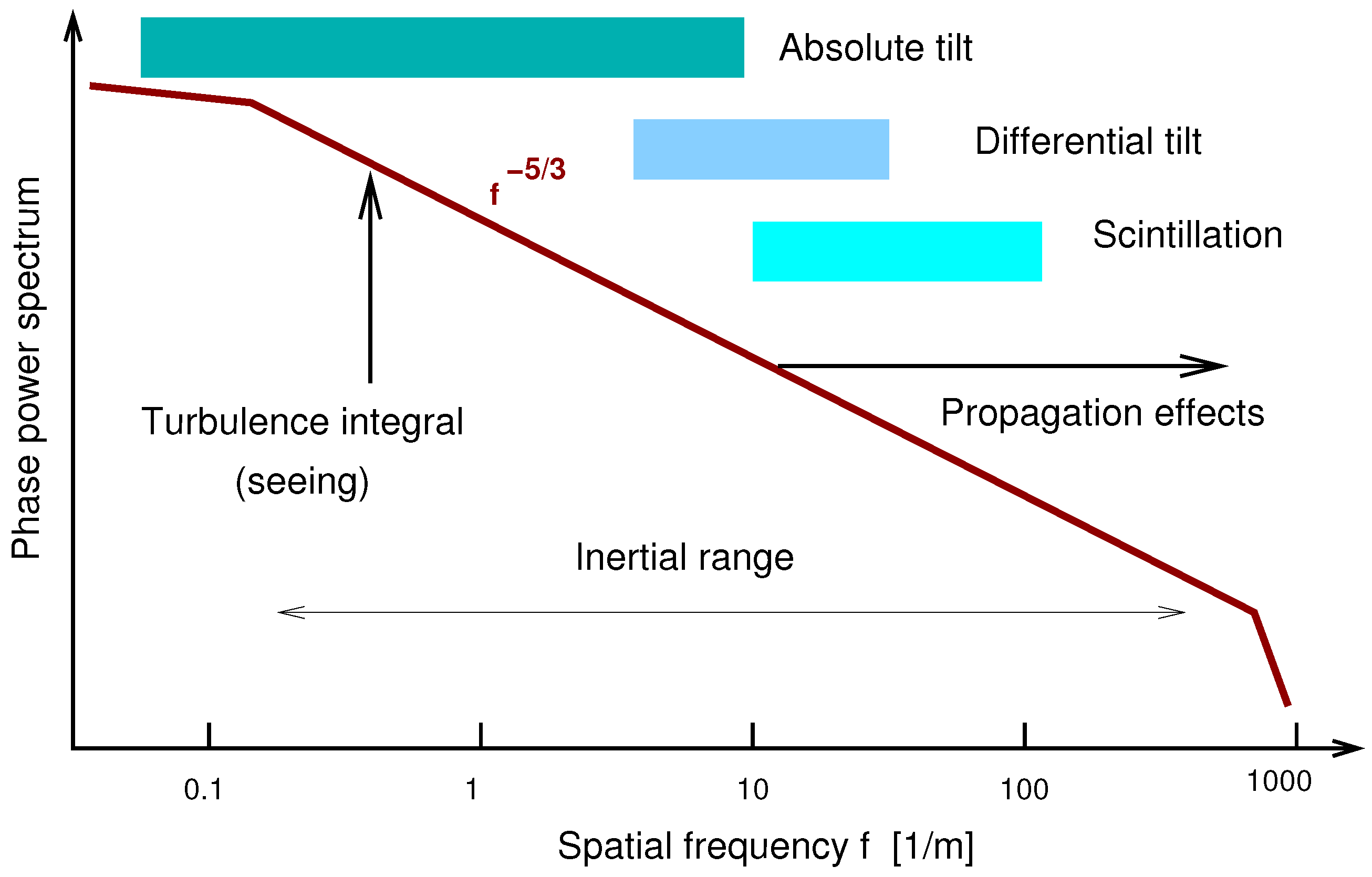
To summarize this Section, Table 2 lists various types of seeing monitors, the measured quantities, advantages and pitfalls of each approach. All monitors are based on the standard theory, hence on the assumption that atmospheric distortions are a stationary process with a Kolmogorov spectrum (Figure 1). Each instrument samples a certain portion of this spectrum by measuring covariance of some optical parameter, and deduces a single quantity that describes the total turbulence strength, hence seeing. The following Section confronts this theoretical landscape with reality.
4. Limitations of the Seeing Concept
The operation of a modern observatory critically depends on the information on seeing delivered by site monitors. Observers typically assume that these data allow for the accurate prediction of the image quality in a telescope (after standard corrections for wavelength dependence and zenith distance) that looks through a uniformly turbulent atmosphere envisioned by the standard theory. In reality, turbulence is not uniform and resembles clouds that cross the line of sight randomly, so the telescope and the site monitor experience different “seeings”. Spatial and temporal non-stationarity of the turbulence (called intermittency in the atmospheric physics) is a significant factor. The largest instability is usually encountered in the lowest layers near the surface (SL—surface layer), which often also significantly contributes to the seeing. Therefore, a difference in location and height between the site monitor tower and the telescope translates into a difference between respective seeing values. Experimental evidence for intermittency and SL variations is gathered in the rest of this Section.
4.1. Seeing Variability
Soundings of the atmosphere by balloons with micro-thermal sensors reveal typical spikes of temperature fluctuations at certain altitudes [21]. They were originally interpreted as very thin turbulent layers. Groups of such layers are concentrated at the interface between zones with different temperatures and wind speeds, where intensive mixing creates temperature fluctuations [55]. The thickness of the mixing zone might be a few hundred meters. Turbulence spikes with a typical size of ∼20 m do not necessarily correspond to thin horizontally stratified layers; more likely, they are just cloudlets of strong turbulence. A single pass of a balloon cannot distinguish between flat or cloud-like geometries of these zones.
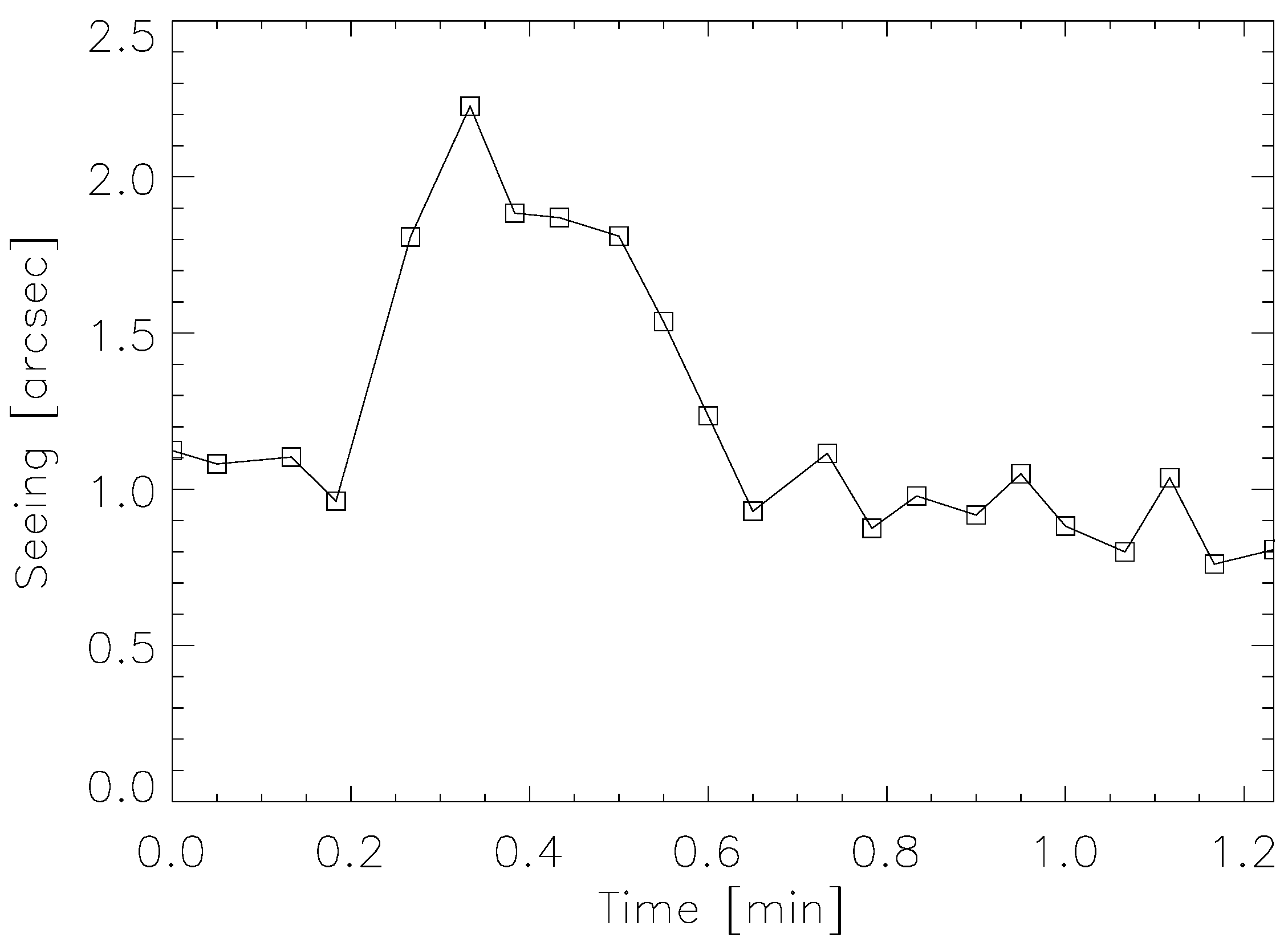
In some seeing monitors (e.g., MASS, RINGSS), variance of the optical quantities is computed on short time intervals and then averaged over a longer time on the order of a minute. Seeing and other parameters are deduced from the average variance for a good reason: the relation between the measured (variance) and derived (turbulence integral) parameters is linear, so in theory the order of averaging is not important. However, restoration of turbulence profile imposes non-negativity of , which introduces a non-linearity, and in such case the averaging order does matter. This said, availability of the high-cadence data allows us to probe fast seeing variations. Kornilov [56] established that the variance of scintillation indices in MASS recorded every second is substantially larger than expected for a stationary process, indicating fast variability of turbulence strength. The same conclusion is reached from the analysis of the individual data cubes in RINGSS: the variance of measured parameters is substantially larger compared to simulated data with stationary turbulence. Figure 2 shows a short seeing spike recorded at Paranal (seeing was derived here from the individual 2 s data cubes, 2000 frames each, recorded with a cadence of ∼4 s). The shape of the spike shows that it is not an instrumental glitch (indeed, the quality parameters are good for all these data). Turbulence causing this spike was localized at heights between 0.5 and 1 km; its duration of 20 s and the wind speed of 5 m indicate that the size of this turbulent cloud was on the order of 100 m.
Typically, site monitors measure seeing with a cadence of ∼1 min. Extensive series of accumulated seeing data allow for detailed studies of its temporal variability [57,58]. Changes on time scales from minutes to hours are typical. Intermittency of optical turbulence also implies dependence of the seeing on the viewing direction. So, ground-based telescopes do not look though a homogeneous medium with a horizontally stratified and slowly evolving profile, but rather deal with a highly dynamical situation where the seeing depends on the viewing direction and can change rapidly. The fact that seeing depends on the integrated effect of the whole atmosphere somewhat reduces its variability, except in situations where one strong layer dominates. So, the seeing can be relatively stable on some nights but quite “spiky” on other nights. Similarly, telescopes looking in different directions will experience different seeing conditions, and this difference can vary from negligible to major, depending on the night.
Seeing variability limits the accuracy of its measurement. The variance of some optical parameters used to estimate the seeing (e.g., a differential tilt) can have a relative statistical error of or larger, where N is the number of independent samples. If images in a DIMM are acquired at a rate of 100 Hz and samples are collected in a minute, the variance can be measured with almost a percent statistical error, at least in principle. In reality, the samples are not independent (correlated), while the major contributor to the uncertainly is turbulence non-stationarity. Statistical error of seeing measurement by a given instrument determined using simulated data can serve as a lower-limit error estimate. An upper limit (biased by fast seeing variability) can be evaluated by comparing sequential seeing data points. Looking at the plot in Figure 2, one can see that after the spike, sequential values agree within ∼15%. Measuring seeing with an error of a percent is an illusory and unachievable goal: while we accumulate the statistics, the seeing has already changed!
4.2. Unstable Surface Layer
The surface layer (SL) is the most unstable and unpredictable part of the atmosphere. Local turbulence in the night-time SL can be measured by acoustic sounding (e.g., [59]), by micro-thermal probes [13], or, preferably, by optical instruments like SLODAR [60] or lunar scintillometers [61]. A scintillometer pointed to a large source like the Moon records very small fluctuations of the flux, and their covariance yields a low-resolution turbulence profile in the range from a few to a few hundred meters. Data collected at several sites evidence extreme variability of the SL. Averaged over a long time, the SL profile can be approximated by a negative exponent [59] or by a power law like (see Figure 4 in [62]). The integral of an power law diverges at both low and upper limits, so its value depends on the adopted SL limits.
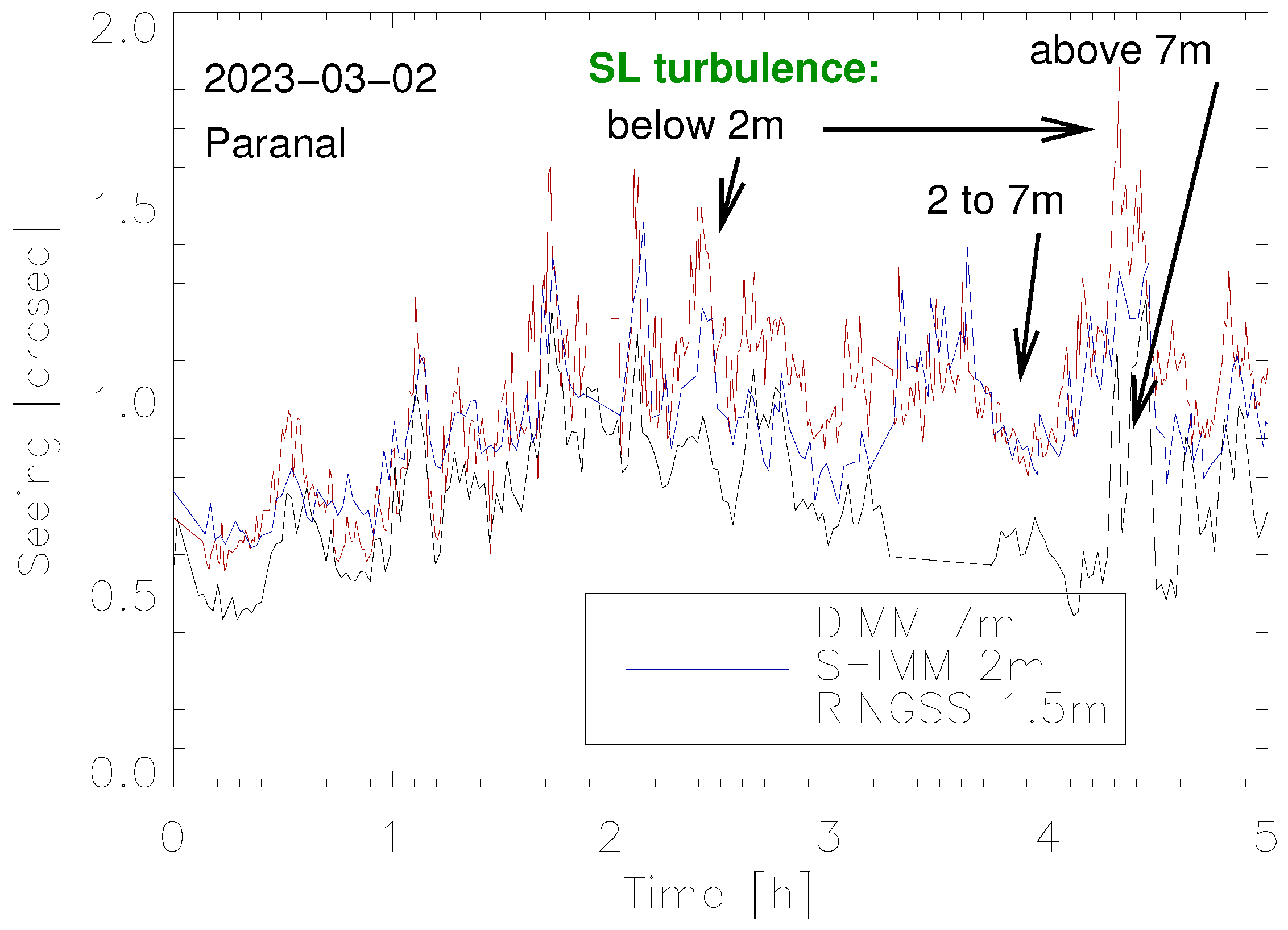
The contribution of SL to the overall seeing can be appreciated from the example shown in Figure 3. Three seeing monitors working simultaneously show a good overall agreement, while the systematic differences can be explained by the SL contribution. At times the SL is so strong and thin that instruments installed at 1.5 and 2 m above ground measure a different seeing. However, at other times the RINGSS and SHIMM agree very well, while DIMM, installed higher, still measures a better seeing. After 4 h, the DIMM also recorded spikes in seeing caused by the SL. On the other hand, the seeing spike at 0.5 h, registered by all three monitors, was produced by a high turbulence.
Another common way to quantify the turbulence in the few hundred meters above ground is by comparing the full seeing measured by a DIMM with the free-atmosphere seeing measured by MASS simultaneously, pointing at the same star. The turbulence integral is proportional to , so the SL seeing is estimated as
Considering numerous biases of both instruments and random errors, situations when are not uncommon; in such cases we set .
The simultaneous operation of both a MASS-DIMM monitor and a lunar scintillometer revealed that the SL turbulence can be weaker than implied by the differentially estimated , raising concerns about reliability of the DIMM seeing. Data from various sources assembled in [62] indicate that typical values of the SL turbulence integral between, say, 6 m and 100 m, are around according to lunar scintillometers or micro-thermal probes, but around if measured by a MASS-DIMM instrument on the same site simultaneously (see also [63]). This discrepancy can be attributed to local effects in a DIMM, such as optical distortions generated by the telescope and its enclosure (those can be considered as effectively reducing the height of an instrument above ground) or by an opto-mechanical instability causing slow but measurable changes in the separation between the two spots, e.g., due to temperature variations in the focus or other deformations. In contrast, a lunar scintillometer starts to sense turbulence only at a distance of a few meters and is therefore immune to the local distortions.
Optical fluctuations of air inside telescope enclosures are known as dome seeing. Under good conditions, their contribution to the image degradation can be substantial. In a SCIDAR, the dome seeing is often evaluated and subtracted, taking advantage of the fact that dome turbulence evolves much slower than the atmospheric one. In analogy to the dome seeing, optical distortions can arise in the vicinity of a site monitor, biasing the seeing measurements. So, the design of the site monitor tower and enclosure and the nearby heat sources such as power supplies and computers can affect (increase) the measured seeing.
The importance of local effects has been demonstrated by the comparison between two seeing monitors installed at Cerro Tololo within a few meters from each other, at the same height above ground [64]. The old DIMM tower was a cylinder, while the new DIMM tower was a truss transparent to the wind. Furthermore, the old tower was located closer to the edge of the platform where the incoming wind likely created rising “plumes” of turbulence. The systematic difference between the two DIMMs was found to depend on the wind direction. It is not recommended to install a site monitor tower near the edge of the observatory platform facing the wind, where a sharp cliff generates additional local turbulence.
The discrepancy between DIMM seeing and telescope PSF at Paranal has been attributed to the strong SL and to the local effects around the original site monitor installed near the edge at a 3 m height [65]. The new site monitor was re-located further from the edge after a detailed investigation of the local turbulence using lunar scintillometers and other instruments [66].
Strong vertical temperature gradients in the SL and mixing by the wind shear are the cause of the strong optical turbulence. The near-ground turbulence is known to be anisotropic, where the structure function depends on the direction of (a faster growth in the vertical direction compared to horizontal). In such situation, a single value of the parameter does not suffice to model the distortions, and the standard (isotropic) model, on which the seeing concept is based, becomes even more questionable. Furthermore, refractive-index fluctuations in the SL and in the vicinity of the site monitor can be of a non-turbulent origin, caused by, e.g., gravity waves or by a quasi-laminar air flow with temperature gradients.
5. Summary
The concept of seeing is based on the idealized model of optical turbulence, representing it by a stationary random process with an isotropic Kolmogorov spectrum. In reality, the turbulence is intermittent, and the model holds only approximately within certain air volumes and certain time intervals. The turbulence intensity (hence seeing) depends on location, viewing direction, and, of course, on time. Optical turbulence resembles random clouds rather than a uniform “sea” of refractive-index fluctuations with homogeneous statistics. Intermittency is a fundamental characteristic of atmospheric turbulence which limits our ability to average its intensity over space and time. So, the data of seeing monitors are estimates rather than accurate measurements. Substantial variations in seeing on time scales from minutes to years have been demonstrated; the long-term seeing variability is driven by climate cycles associated with changing wind patterns.
Optical seeing monitors record some optical effects caused by the turbulence (e.g., wave-front curvature or intensity fluctuations), process the results statistically, and interpret them in terms of seeing within the framework of the standard model. Non-stationarity of the turbulence puts a limit to the sample size: the longer we accumulate, the less stable is the measured parameter, seeing.
Each seeing monitor samples wave-front fluctuations in a certain range of spatial scales and is burdened by several biases of both fundamental nature (finite exposure time, detector noise, propagation) and those arising from instrumental imperfections (e.g., poor focusing in a DIMM, wind shake). Fundamental biases should be modeled and accounted for using simulations. Instrumental biases can be reduced to an acceptable level by careful control of critical parameters. Two well-maintained seeing monitors should agree to a level of ∼10%; seeking a better agreement might prove illusory owing to the approximate nature of seeing.
Even though the seeing data are never very accurate in the absolute sense, their utility for observatory operation is unquestionable. Distinguishing between good, typical, and poor seeing conditions and adjusting the programs accordingly is a great resource for improving efficiency of modern observatories. Such a practice is in place at the VLT and Gemini telescopes.
The selection of astronomical sites and their inter-comparison in terms of seeing is a more delicate matter. Using identical sets of seeing monitors is always recommended. However, it is also essential to ensure a good correction of biases because they depend on the site parameters such as wind speed or fraction of high turbulence. The comparison between sites based on identical but biased seeing monitors is a questionable strategy. Likewise, “calibrating” site monitors against each other and adopting some instrument as a standard or a reference is a futile approach. Instead, we should think of inter-comparison between site monitors as a useful check of their correctness (e.g., [67]). So far, the best example of a site-comparison campaign is the selection of the site for the Thirty Meter Telescope, TMT [4]. With the increasing role of AO, such parameters as wind speed and free-atmosphere seeing gain more weight compared to the total seeing. The selected TMT site, Mauna Kea, does not rank first in total seeing among the six candidates. Still, this is a wise choice, considering the intrinsically uncertain nature of the seeing discussed in this review.
Seeing at the Paranal observatory, site of the VLT, is an illustrative story. Before selecting this site, its excellent seeing had been established by a DIMM installed on a 3 m tower and working for several years. However, when the site monitor resumed operation after the telescopes were constructed, the measured seeing notably degraded. Furthermore, it was found that image quality in the VLT was often better than predicted by a DIMM. The reason of this discrepancy was finally established: it was caused by the unfortunate location of the DIMM near the edge of the platform in a low 3 m tower and by the changing wind pattern [65]. The new Paranal site monitor in a 7 m tower measures a systematically better seeing, although it is still occasionally affected by the SL (Figure 3).
The DIMM, universally adopted as a standard method of measuring seeing, remains valid. However, additional information on the turbulence location and its characteristic time offered by the MASS-DIMM instruments has proven to be of value, especially for operation of the AO systems. The uncertainty of seeing caused by the highly variable SL is partially offset by estimates of the free-atmosphere seeing. By comparing those two estimates, pessimistic and optimistic, a better idea of the “true” seeing can be gained. To address the technical obsolescence of MASS, the RINGSS and FASS instruments have been developed. Alternatively, DIMM extensions based on the Shack-Hartmann idea (SHIMM) can be used.
Looking into the future, the demand for reliable and unbiased seeing monitors will persist. Naturally, seeing monitors operate robotically, without human assistance. However, they still require manpower for maintenance, quality control, data management, and repairs. For these activities, local staff with a certain skill set is needed. The most frequent failures relate to such generic subsystems as enclosure, mount, and computers. Thus, the “cost of ownership” over many years can surpass the initial investment in the construction of a seeing monitor.
To reduce the cost of ownership of a seeing monitor, attention should be paid to the robustness and reliability of its critical subsystems, in particular the enclosure and the mount. Using smaller, more compact optics helps the reliability and, at the same time, diminishes the local air disturbances caused by the instrument. Ideally, a site monitor should be a self-contained unit with fully robotic operation, including self-diagnostic. Data processing and distribution should also be part of the package. Instruments like DIMM, RINGSS or SHIMM can be assembled from commercial parts and use a shared software, but this does not reduce the cost of their ownership.
Modern cars are much more complex than site monitors, and yet most people use cars without knowing details of their interior operation—a result of extensive car engineering. It is unrealistic to expect a comparable level of engineering effort being invested in seeing monitors, owing to the much smaller market. Commercially available self-contained seeing monitors of the “set and forget” type are technically feasible, but they are unlikely to appear in the near-term because of the small user base.
Funding
This research was funded by the NSF’s NOIRLab.
Acknowledgments
I am grateful to my thesis advisor Peter Sheglov for raising my initial interest and motivation in site testing. Collaboration with my colleagues A. Gur’yanov, F. Martin, V. Kornilov, M. Sarazin, E. Bustos, and many others was an enriching and productive experience during many years. This work used bibliographic references from the Astrophysics Data System maintained by SAO/NASA.
Conflicts of Interest
The author declares no conflict of interest.
References
- Young, A.T. Seeing: Its Cause and Cure. Astrophys. J. 1974, 189, 587–604. [Google Scholar] [CrossRef]
- Coulman, C.E. Fundamental and applied aspects of astronomical “seeing”. Annu. Rev. Astron. Astrophys. 1985, 23, 19–57. [Google Scholar] [CrossRef]
- Racine, R.; Salmon, D.; Cowley, D.; Sovka, J. Mirror, Dome, and Natural Seeing at CFHT. Publ. Astron. Soc. Pac. 1991, 103, 1020–1032. [Google Scholar] [CrossRef]
- Schöck, M.; Els, S.; Riddle, R.; Skidmore, W.; Travouillon, T.; Blum, R.; Bustos, E.; Chanan, G.; Djorgovski, S.G.; Gillett, P.; et al. Thirty Meter Telescope Site Testing I: Overview. Publ. Astron. Soc. Pac. 2009, 121, 384–395. [Google Scholar] [CrossRef]
- Kuiper, G.P.; Middlehurst, B.M. Telescopes; Chicago Univercity Press: Chicago, IL, USA, 1961. [Google Scholar]
- Tatarskii, V.I. Wave Propagation in Turbulent Medium; McGraw-Hill: New York, NY, USA, 1961. [Google Scholar]
- Babcock, H.W. Instrumental Recording of Astronomical Seeing. Publ. Astron. Soc. Pac. 1963, 75, 1–8. [Google Scholar] [CrossRef]
- Harlan, E.A.; Walker, M.F. A Star-Trail Telescope for Astronomical Site-Testing. Publ. Astron. Soc. Pac. 1965, 77, 246–252. [Google Scholar] [CrossRef]
- Stock, J.; Keller, G. Telescopes; Kuiper, G.P., Middlehurst, B.M., Eds.; Chicago University Press: Chicago, IL, USA, 1961; pp. 138–153. [Google Scholar]
- Fried, D.L. Differential angle of arrival—Theory, evaluation, and measurement feasibility. Radio Sci. 1975, 10, 71–76. [Google Scholar] [CrossRef]
- Dainty, J.C.; Scaddan, R.J. A coherence interferometer for direct measurement of the atmospheric transfer function. Mon. Not. R. Astron. Soc. 1974, 167, 69P–74P. [Google Scholar] [CrossRef]
- Kovadlo, P.G.; Shikhovtsev, A.Y.; Kopylov, E.A.; Kiselev, A.V.; Russkikh, I.V. Study of the Optical Atmospheric Distortions using Wavefront Sensor Data. Russ. Phys. J. 2021, 63, 1952–1958. [Google Scholar] [CrossRef]
- Zhu, L.; Zhang, H.; Zhang, L.; Duan, X.; Lu, X.; Liu, Y.; Li, X.; Sun, G.; Weng, N. Astronomical seeing and ground-level optical turbulence at Delingha observatory on the northern Tibetan Plateau. Mon. Not. R. Astron. Soc. 2023, 525, 3236–3247. [Google Scholar] [CrossRef]
- Shikhovtsev, A.Y.; Kovadlo, P.G.; Kiselev, A.V.; Eselevich, M.V.; Lukin, V.P. Application of Neural Networks to Estimation and Prediction of Seeing at the Large Solar Telescope Site. Publ. Astron. Soc. Pac. 2023, 135, 014503. [Google Scholar] [CrossRef]
- Roddier, F. The effects of atmospheric turbulence in optical astronomy. Prog. Opt. 1981, 19, 281–376. [Google Scholar] [CrossRef]
- Sasiela, R.J. Electromagnetic Wave Propagation in Turbulence. Evaluation and Application of Mellin Transforms; Springer: Berlin/Heidelberg, Germany, 1994. [Google Scholar]
- Goodman, J.W. Statistical Optics; Wiley-VCH: Weinheim, Germany, 2000. [Google Scholar]
- Fried, D.L. Optical Resolution Through a Randomly Inhomogeneous Medium for Very Long and Very Short Exposures. J. Opt. Soc. Am. 1966, 56, 1372–1379. [Google Scholar] [CrossRef]
- Tokovinin, A. From Differential Image Motion to Seeing. Publ. Astron. Soc. Pac. 2002, 114, 1156–1166. [Google Scholar] [CrossRef]
- Floyd, D.J.E.; Thomas-Osip, J.; Prieto, G. Seeing, Wind, and Outer Scale Effects on Image Quality at the Magellan Telescopes. Publ. Astron. Soc. Pac. 2010, 122, 731–742. [Google Scholar] [CrossRef]
- Azouit, M.; Vernin, J. Optical Turbulence Profiling with Balloons Relevant to Astronomy and Atmospheric Physics. Publ. Astron. Soc. Pac. 2005, 117, 536–543. [Google Scholar] [CrossRef]
- Hardy, J.W. Adaptive Optics for Astronomical Telescopes; Oxford University Press: Oxford, UK, 1998. [Google Scholar]
- Roddier, F. Adaptive Optics in Astronomy; Cambridge University Press: Cambridge, UK, 1999. [Google Scholar]
- Tyson, R.K. Introduction to Adaptive Optics; SPIE Press: Bellingham, WA, USA, 2000. [Google Scholar]
- Noll, R.J. Zernike polynomials and atmospheric turbulence. J. Opt. Soc. Am. 1976, 66, 207–211. [Google Scholar] [CrossRef]
- Roddier, C.; Roddier, F. Correlation measurements on the complex amplitude of stellar plane waves perturbed by atmospheric turbulence. J. Opt. Soc. Am. 1973, 63, 661–663. [Google Scholar] [CrossRef]
- Tokovinin, A.A. An interferometer for determining the modulation transfer function of the atmosphere. Sov. Astron. Lett. 1978, 4, 229–230. [Google Scholar]
- Tokovinin, A.A. Coherence Interferometer with a Lloyd Mirror for Seeing Measurements. Astron. Tsirkulyar 1985, 1366, 4. [Google Scholar]
- Martin, H.M. Image motion as a measure of seeing quality. Publ. Astron. Soc. Pac. 1987, 99, 1360–1370. [Google Scholar] [CrossRef]
- Sarazin, M.; Roddier, F. The ESO differential image motion monitor. Astron. Astrophys. 1990, 227, 294–300. [Google Scholar]
- Akbari, L.; Darudi, A.; Shomali, R. Atmospheric coherence time measurement by modified Fast Defocus method. Optik 2021, 233, 166494. [Google Scholar] [CrossRef]
- Tokovinin, A.; Kornilov, V. Accurate seeing measurements with MASS and DIMM. Mon. Not. R. Astron. Soc. 2007, 381, 1179–1189. [Google Scholar] [CrossRef]
- Berdja, A.; Borgnino, J.; Irbah, A. Fresnel diffraction and polychromatic effects on angle-of-arrival fluctuations. J. Opt. Pure Appl. Opt. 2006, 8, 244–251. [Google Scholar] [CrossRef]
- Kornilov, V.; Safonov, B. Wave propagation effect on differential image motion monitor measurements. Mon. Not. R. Astron. Soc. 2019, 488, 1273–1281. [Google Scholar] [CrossRef]
- Kornilov, V.; Safonov, B. Differential image motion in the short-exposure regime. Mon. Not. R. Astron. Soc. 2011, 418, 1878–1888. [Google Scholar] [CrossRef]
- Gur’yanov, A.E.; Kallistratova, M.A.; Kutyrev, A.S.; Petenko, I.V.; Shcheglov, P.V.; Tokovinin, A.A. The contribution of the lower atmospheric layers to the seeing at some mountain observatories. Astron. Astrophys. 1992, 262, 373–381. [Google Scholar]
- Ziad, A.; Conan, R.; Tokovinin, A.; Martin, F.; Borgnino, J. From the Grating Scale Monitor to the Generalized Seeing Monitor. Appl. Opt. 2000, 39, 5415–5425. [Google Scholar] [CrossRef]
- Vernin, J.; Azouit, M. Image processing adapted to the atmospheric speckle. II. Remote sounding of turbulence by means of multidimensional analysis. J. Opt. 1983, 14, 131–142. [Google Scholar] [CrossRef]
- Klueckers, V.A.; Wooder, N.J.; Nicholls, T.W.; Adcock, M.J.; Munro, I.; Dainty, J.C. Profiling of atmospheric turbulence strength and velocity using a generalised SCIDAR technique. Astron. Astrophys. Suppl. 1998, 130, 141–155. [Google Scholar] [CrossRef]
- Avila, R.; Vernin, J.; Sánchez, L.J. Atmospheric turbulence and wind profiles monitoring with generalized scidar. Astron. Astrophys. 2001, 369, 364–372. [Google Scholar] [CrossRef]
- Shepherd, H.W.; Osborn, J.; Wilson, R.W.; Butterley, T.; Avila, R.; Dhillon, V.S.; Morris, T.J. Stereo-SCIDAR: Optical turbulence profiling with high sensitivity using a modified SCIDAR instrument. Mon. Not. R. Astron. Soc. 2014, 437, 3568–3577. [Google Scholar] [CrossRef]
- Butterley, T.; Sarazin, M.; Le Louarn, M.; Osborn, J.; Farley, O.J.D. Correction of finite spatial and temporal sampling effects in stereo-SCIDAR. In Proceedings of the Adaptive Optics Systems VII; Schreiber, L., Schmidt, D., Vernet, E., Eds.; Society of Photo-Optical Instrumentation Engineers (SPIE) Conference Series; Society of Photo-Optical Instrumentation Engineers (SPIE): Bellingham, WA, USA, 2020; Volume 11448, p. 114481W. [Google Scholar] [CrossRef]
- Ochs, G.R.; Wang, T.I.; Lawrence, R.S.; Clifford, S.F. Refractive-turbulence profiles measured by one-dimensional spatial filtering of scintillations. Appl. Opt. 1976, 15, 2504–2510. [Google Scholar] [CrossRef]
- Caccia, J.L.; Azouit, M.; Vernin, J. Wind and C(N)-squared profiling by single-star scintillation analysis. Appl. Opt. 1987, 26, 1288–1294. [Google Scholar] [CrossRef]
- Tokovinin, A.A. A new method of measuring atmospheric seeing. Astron. Lett. 1998, 24, 662–664. [Google Scholar]
- Kornilov, V.; Tokovinin, A.A.; Vozyakova, O.; Zaitsev, A.; Shatsky, N.; Potanin, S.F.; Sarazin, M.S. MASS: A monitor of the vertical turbulence distribution. In Proceedings of the Adaptive Optical System Technologies II; Wizinowich, P.L., Bonaccini, D., Eds.; Society of Photo-Optical Instrumentation Engineers (SPIE) Conference Series; Society of Photo-Optical Instrumentation Engineers (SPIE): Bellingham, WA, USA, 2003; Volume 4839, pp. 837–845. [Google Scholar] [CrossRef]
- Tokovinin, A.A. Polychromatic scintillation. J. Opt. Soc. Am. A 2003, 20, 686–689. [Google Scholar] [CrossRef]
- Kornilov, V.; Tokovinin, A.; Shatsky, N.; Voziakova, O.; Potanin, S.; Safonov, B. Combined MASS-DIMM instruments for atmospheric turbulence studies. Mon. Not. R. Astron. Soc. 2007, 382, 1268–1278. [Google Scholar] [CrossRef]
- Robert, C.; Conan, J.M.; Michau, V.; Fusco, T.; Vedrenne, N. Scintillation and phase anisoplanatism in Shack-Hartmann wavefront sensing. J. Opt. Soc. Am. A 2006, 23, 613–624. [Google Scholar] [CrossRef]
- Ogane, H.; Akiyama, M.; Oya, S.; Ono, Y. Atmospheric turbulence profiling with multi-aperture scintillation of a Shack–Hartmann sensor. Mon. Not. R. Astron. Soc. 2021, 503, 5778–5788. [Google Scholar] [CrossRef]
- Potanin, S.A.; Kornilov, M.V.; Savvin, A.D.; Safonov, B.S.; Ibragimov, M.A.; Kopylov, E.A.; Nalivkin, M.A.; Shmagin, V.E.; Huy, L.X.; Thao, N.T. A Facility for the Study of Atmospheric Parameters Based on the Shack–Hartmann Sensor. Astrophys. Bull. 2022, 77, 214–221. [Google Scholar] [CrossRef]
- Griffiths, R.; Osborn, J.; Farley, O.; Butterley, T.; Townson, M.J.; Wilson, R. Demonstrating 24-hour continuous vertical monitoring of atmospheric optical turbulence. Optics Express 2023, 31, 6730–6740. [Google Scholar] [CrossRef] [PubMed]
- Tokovinin, A. Measurement of turbulence profile from defocused ring images. Mon. Not. R. Astron. Soc. 2021, 502, 794–808. [Google Scholar] [CrossRef]
- Guesalaga, A.; Ayancán, B.; Sarazin, M.; Wilson, R.W.; Perera, S.; Le Louarn, M. FASS: A turbulence profiler based on a fast, low-noise camera. Mon. Not. R. Astron. Soc. 2021, 501, 3030–3045. [Google Scholar] [CrossRef]
- Coulman, C.E.; Vernin, J.; Fuchs, A. Optical seeing-mechanism of formation of thin turbulent laminae in the atmosphere. Appl. Opt. 1995, 34, 5461–5474. [Google Scholar] [CrossRef]
- Kornilov, V. Stellar scintillation in the short exposure regime and atmospheric coherence time evaluation. Astron. Astrophys. 2011, 530, A56. [Google Scholar] [CrossRef]
- Racine, R. Temporal Fluctuations of Atmospheric Seeing. Publ. Astron. Soc. Pac. 1996, 108, 372–374. [Google Scholar] [CrossRef]
- Vernin, J.; Muñoz-Tuñón, C. The temporal behaviour of seeing. New Astron. Rev. 1998, 42, 451–454. [Google Scholar] [CrossRef]
- Tokovinin, A.; Travouillon, T. Model of optical turbulence profile at Cerro Pachón. Mon. Not. R. Astron. Soc. 2006, 365, 1235–1242. [Google Scholar] [CrossRef]
- Wilson, R.W. SLODAR: Measuring optical turbulence altitude with a Shack-Hartmann wavefront sensor. Mon. Not. R. Astron. Soc. 2002, 337, 103–108. [Google Scholar] [CrossRef]
- Tokovinin, A.; Bustos, E.; Berdja, A. Near-ground turbulence profiles from lunar scintillometer. Mon. Not. R. Astron. Soc. 2010, 404, 1186–1196. [Google Scholar] [CrossRef]
- Tokovinin, A. Where is the surface-layer turbulence? In Proceedings of the Ground-based and Airborne Telescopes III; Stepp, L.M., Gilmozzi, R., Hall, H.J., Eds.; Society of Photo-Optical Instrumentation Engineers (SPIE) Conference Series; Society of Photo-Optical Instrumentation Engineers (SPIE): Bellingham, WA, USA, 2010; Volume 7733, p. 77331N. [Google Scholar] [CrossRef]
- Els, S.G.; Travouillon, T.; Schöck, M.; Riddle, R.; Skidmore, W.; Seguel, J.; Bustos, E.; Walker, D. Thirty Meter Telescope Site Testing VI: Turbulence Profiles. Publ. Astron. Soc. Pac. 2009, 121, 527–543. [Google Scholar] [CrossRef]
- Els, S.G.; Schöck, M.; Bustos, E.; Seguel, J.; Vasquez, J.; Walker, D.; Riddle, R.; Skidmore, W.; Travouillon, T.; Vogiatzis, K. Four Years of Optical Turbulence Monitoring at the Cerro Tololo Inter-American Observatory (CTIO). Publ. Astron. Soc. Pac. 2009, 121, 922–934. [Google Scholar] [CrossRef]
- Sarazin, M.; Melnick, J.; Navarrete, J.; Lombardi, G. Seeing is Believing: New Facts about the Evolution of Seeing on Paranal. Messenger 2008, 132, 11–17. [Google Scholar]
- Lombardi, G.; Melnick, J.; Hinojosa Goñi, R.H.; Navarrete, J.; Sarazin, M.; Berdja, A.; Tokovinin, A.; Wilson, R.; Osborn, J.; Butterley, T.; et al. Surface layer characterization at Paranal Observatory. In Proceedings of the Ground-Based and Airborne Telescopes III; Stepp, L.M., Gilmozzi, R., Hall, H.J., Eds.; Society of Photo-Optical Instrumentation Engineers (SPIE) Conference Series; Society of Photo-Optical Instrumentation Engineers (SPIE): Bellingham, WA, USA, 2010; Volume 7733, p. 77334D. [Google Scholar] [CrossRef]
- Dali Ali, W.; Ziad, A.; Berdja, A.; Maire, J.; Borgnino, J.; Sarazin, M.; Lombardi, G.; Navarrete, J.; Vazquez Ramio, H.; Reyes, M.; et al. Multi-instrument measurement campaign at Paranal in 2007. Characterization of the outer scale and the seeing of the surface layer. Astron. Astrophys. 2010, 524, A73. [Google Scholar] [CrossRef]
Figure 1.
Schematic representation of the spatial spectrum of phase distortions in the standard model. It is proportional to in the inertial range between a few meters and a few millimeters, and the proportionality coefficient determines the seeing. Seeing monitors sample different regions of this spectrum, depending on the measured parameters. Absolute tilts are sensitive to large scales, differential tilts sense a narrow range around 0.1 m, and scintillation probes even smaller scales where the propagation effects become important, affecting both phase and amplitude of the light waves.

Figure 2.
Fragment of high-cadence seeing data at Paranal observatory measured on 5 March 2023 at 0:26 UT with the RINGSS instrument.
Figure 2.
Fragment of high-cadence seeing data at Paranal observatory measured on 5 March 2023 at 0:26 UT with the RINGSS instrument.

Figure 3.
Evolution of seeing at Paranal during five hours measured by three different instruments: a regular DIMM, SHIMM, and RINGSS. The SHIMM data are provided by R. Griffiths.
Figure 3.
Evolution of seeing at Paranal during five hours measured by three different instruments: a regular DIMM, SHIMM, and RINGSS. The SHIMM data are provided by R. Griffiths.


Table 1.
Seeing parameters.
| Parameter | Units | Conversion | ||
|---|---|---|---|---|
| Seeing | rad | |||
| Fried radius | m | |||
| Integral | [] |
Table 2.
Types of seeing monitors.
| Type | Measured Effect | Advantages | Problems |
|---|---|---|---|
| Interferometer | Coherence function | Theoretically perfect | Wind shake |
| Image motion | Tilt | Easy | Wind shake, propagation |
| DIMM | Curvature | Immune to shake | Propagation |
| SCIDAR | Scintillation of double star | Turbulence profile | Large aperture, faint stars |
| MASS | Scintillation | Turbulence profile | Obsolete, expensive |
| SHIMM | Curvature, scintillation | Turbulence profile | Low resolution |
| RINGSS | Scintillation, curvature | Turbulence profile | Small signal |
Disclaimer/Publisher’s Note: The statements, opinions and data contained in all publications are solely those of the individual author(s) and contributor(s) and not of MDPI and/or the editor(s). MDPI and/or the editor(s) disclaim responsibility for any injury to people or property resulting from any ideas, methods, instructions or products referred to in the content. |
© 2023 by the author. Licensee MDPI, Basel, Switzerland. This article is an open access article distributed under the terms and conditions of the Creative Commons Attribution (CC BY) license (https://creativecommons.org/licenses/by/4.0/).
Share and Cite
MDPI and ACS Style
Tokovinin, A. The Elusive Nature of “Seeing”. Atmosphere 2023, 14, 1694. https://doi.org/10.3390/atmos14111694
AMA Style
Tokovinin A. The Elusive Nature of “Seeing”. Atmosphere. 2023; 14(11):1694. https://doi.org/10.3390/atmos14111694
Chicago/Turabian StyleTokovinin, Andrei. 2023. "The Elusive Nature of “Seeing”" Atmosphere 14, no. 11: 1694. https://doi.org/10.3390/atmos14111694
Note that from the first issue of 2016, this journal uses article numbers instead of page numbers. See further details here.