Article

Performance-Based Evaluation of CMIP5 and CMIP6 Global Climate Models and Their Multi-Model Ensembles to Simulate and Project Seasonal and Annual Climate Variables in the Chungcheong Region of South Korea

1
Department of Agricultural Civil Engineering, Kyungpook National University, Daegu 41566, Republic of Korea
2
Department of Agricultural and Biosystems Engineering, University of Ilorin, PMB 1515, Ilorin 240003, Nigeria
3
Institute of Agricultural Science & Technology, Kyungpook National University, Daegu 41566, Republic of Korea
*
Authors to whom correspondence should be addressed.
These authors contributed equally to this work.
Atmosphere 2023, 14(10), 1569; https://doi.org/10.3390/atmos14101569
Submission received: 30 August 2023 / Revised: 27 September 2023 / Accepted: 13 October 2023 / Published: 16 October 2023
(This article belongs to the Special Issue Statistical Approaches in Climatic Parameters Prediction)

Abstract

:
Extreme climate change events are major causes of devastating impacts on socioeconomic well-being and ecosystem damage. Therefore, understanding the performance of appropriate climate models representing local climate characteristics is critical for future projections. Thus, this study analyses the performance of 24 GCMs from the Coupled Model Intercomparison Project Phases 5 and 6 (CMIP5 and 6) and their multi-model ensembles in simulating climate variables including average rainfall, maximum (Tmax), and minimum (Tmin) temperatures at annual and seasonal scales over the Chungcheong region of South Korea from 1975 to 2015. A trend analysis was conducted to estimate the future trends in climate variables in the 2060s (2021–2060) and 2080s (2061–2100). Inverse distance weighting and quantile delta mapping were applied to bias-correct the GCM data. Further, six major evaluating indices comprising temporal and spatial performance assessments were used, after which a comprehensive GCM ranking was applied. The results showed that CMIP6 models performed better in simulating rainfall, Tmax, and Tmin at both temporal and spatial scales. For CMIP5, the top three performing models were GISS, ACCESS1-3, and MRI-CGCM3 for rain; CanESM2, GISS, and MPI-ESM-L-R for Tmax; and GFDL, MRI-CGCM3, and CanESM2 for Tmin. However, the top three performing models in the CMIP6 were MRI-ESM2-0, BCC_CSM, and GFDL for rain; MIROC6, BCC_CSM, and MRI-ESM2-0 for Tmax, and GFDL, MPI_ESM_HR, and MRI-ESM2-0 for Tmin. The multi-model ensembles (an average of the top three GCMs) performed better in simulating rain and Tmin for both CMIP5 and CMIP6 compared with multi-model ensembles (an average of all the GCMs), which only performed slightly better in simulating Tmax. The trend analysis of future projection indicates an increase in rain, Tmax, and Tmin; however, with distinct changes under similar radiative forcing levels in both CMIP5 and CMIP6 models. The projections under RCP4.5 and RCP8.5 increase more than the SSP2-4.5 and SSP5-8.5 scenarios for most climate conditions but are more pronounced, especially for rain, under RCP8.5 than SSP5-8.5 in the far future (2080s). This study provides insightful findings on selecting appropriate GCMs to generate reliable climate projections for local climate conditions in the Chungcheong region of South Korea.

1. Introduction

The frequency, intensity, and duration of climate change impacts such as floods, landslides, drought, and wildfires have increased over the last few decades, causing unabated devastating disasters on society, economy, and ecosystems. Temperature and precipitation (rainfall), important climatic variables for assessing climate change, have witnessed dramatic changes and are projected to be more severe [1]. For instance, in the tropical monsoon region and other territories across the globe, the total human-induced surface air temperature has increased by nearly 1.07 °C (from 0.8 °C to 1.3 °C) between 1850 and 2019. It is projected to become more severe, while the overall precipitation intensity is anticipated to increase under the climate change scenario regarding anthropogenic warning [2]. Similarly, the influence of high emission scenarios could cause a strong Eastern-Pacific type El Niño and consequently impact the precipitation anomaly over East Asia, especially in the northern region [3]. The various natural disasters resulting from extreme climate events are often attributed to unusual changes in climate characteristics [4], causing an overwhelming impact on hydrological facilities and other infrastructures and consequently their failure to protect lives and properties [5].
South Korea is one of the vulnerable countries to climate change that unprecedented natural disasters have recently and continuously impacted due to its geographical location in the tropical monsoon climate region and varying climatic characteristics [4,6,7]. The pattern of extreme climate events in South Korea has become frequent in recent times, such that it causes loss of lives and massive damage to properties [4]. An example of such an event is record-breaking precipitation in 2022, in which up to 141.5 mm of rain per hour occurred mainly in the central region, which resulted in devastating floods and landslides [8]. Similarly, the highest daily maximum temperature was recorded in the summer of 2018 in many parts of East Asia, including South Korea, which caused unprecedented heat waves [9]. Moreover, part of the country is experiencing extreme drought and the worst water scarcity due to low rainfall and intense temperatures [10]. Therefore, there is a need for reliable and accurate information relating to future changes in both precipitation and temperature that could aid policy decision-making toward preparedness and adaptation strategies against climate change impacts.
The global climate models (GCMs) provided by several institutes and international collaborations, such as the Coupled Model Intercomparison Projects (CMIPs), serve as supporting data in the Intergovernmental Panel on Climate Change (IPCC) Assessment Report. The models have also been instrumental in the scientific basis for assessing and evaluating climate change with the most recent outputs from CMIP6. The models in CMIP6 are expected to serve as an improvement and reduce the uncertainty associated with future projections of climate change impacts compared with earlier versions of CMIP5 and CMIP3; still, some studies have indicated otherwise due to the differences in climate variables under investigation and geographical locations [11]. The inconsistency in the simulation results from different models hinders the generalization of GCM performance, thus making it necessary to continue investigating appropriate GCMs that can accurately simulate and project the climate variables of interest in specific regions and local conditions [11].
The performance of 13 GCMs of CMIP6 in simulating historical precipitation and temperature data over Nigeria was assessed [12]. Du et al. compared the performance of precipitation data from CMIP5 and CMIP6 to the observations and found that CMIP6 outperforms CMIP5 in simulating precipitation patterns at a global scale for the historical period [13]. Das et al. investigated the changes in rainfall characteristics relating to tropical monsoon climate from CMIP6 models and found a significant increase in the index value of extreme rainfall [14]. The performances of the GMCs of CMIP5 and CMIP6 for the historical period and future drought projections in South Korea were evaluated [15]. Song et al. also found that CMIP6 models performed well in simulating historical and future daily potential evapotranspiration using climate variables in South Korea [16].
Although many studies have been conducted using GCM data for climate change-related investigations, the simulation and future projection features of extreme events are limited to the national scale and some specific regions. However, to the best of our knowledge, there are currently limited studies on the Chungcheong region of South Korea despite the vulnerability of this region to extreme events of climate change. While the outcomes of GCM studies are essential for climate change impact assessment, complex topographic features and seasonal variability are among the significant factors that affect the accuracy of the results in many regions, including the Chungcheong region, and consequently increase the uncertainties in climate change assessment and projections [17,18]. Meanwhile, an accurate projection of climate variables is crucial for predicting future climate change, especially at the sub-region level, due to their significantly varied impacts associated with a local climate. Furthermore, understanding future projections or trends in essential climate variables like precipitation and temperature could provide a decision-support framework for sustainable water resources management in a region like Chungcheong, where agriculture is the economic mainstay [18]. Thus, it is crucial to comprehensively assess the applicability of GCM models that effectively represent the climatic characteristics of local climates in a region.
This study investigates the appropriateness of GCMs and their multi-model assemblage data from CMIP5 and CMIP6 to simulate historical rain, Tmax, and Tmin and to further estimate future trends in seasonal and annual climate variables at different time slices of the 2060s (2021–2060) and 2080s (2061–2100) in the Chungcheong region of South Korea.

2. Materials and Methods
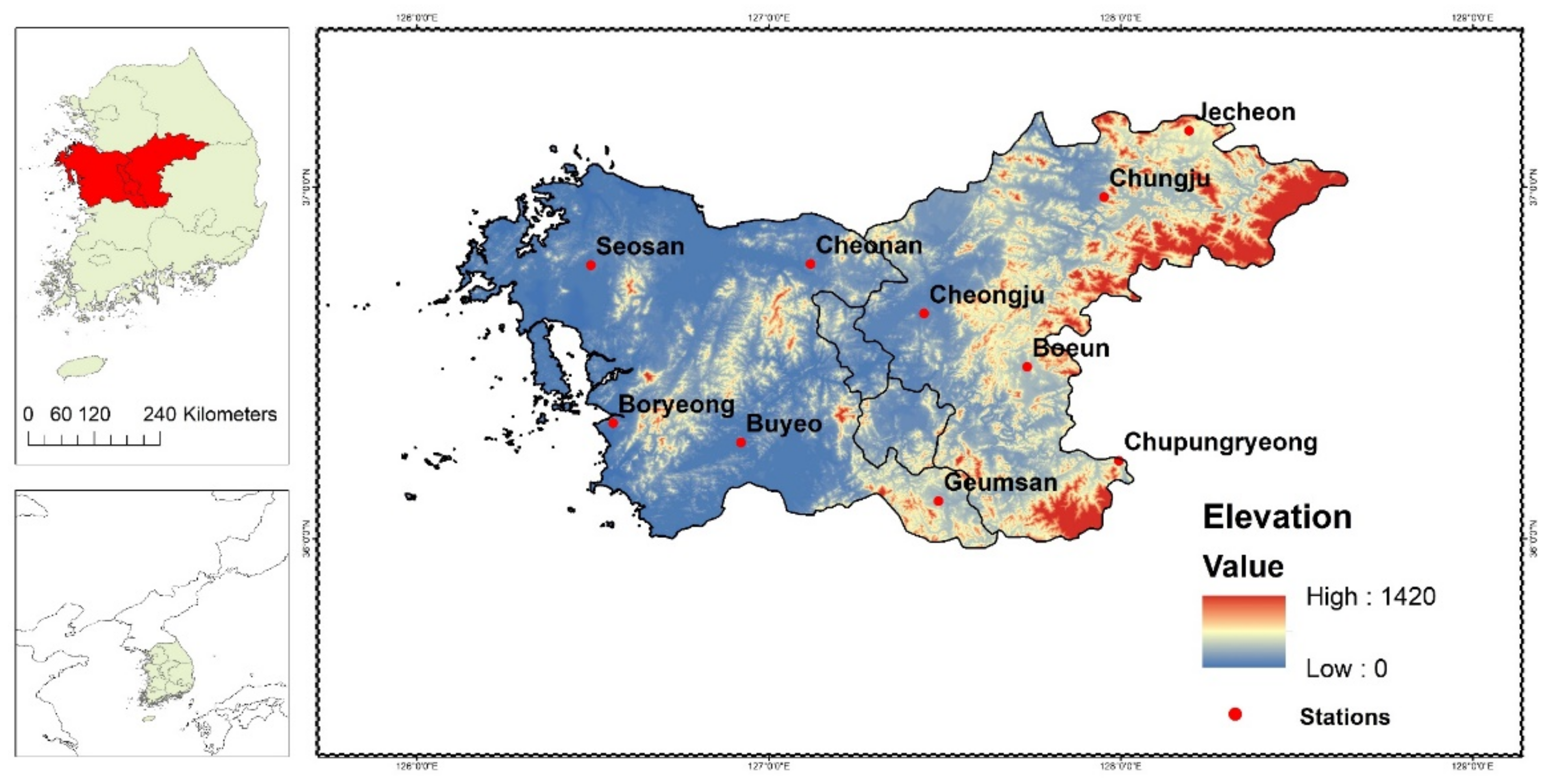
2.1. Study Area

Chungcheong province in South Korea geographically lies between latitude 35°58′ N–36°00′ N and longitude 127°38′ E–125°32′ E in the west-central area of South Korea and on the east end of the Asian continent (Figure 1) [18]. The study area covers about 16,642 km2 with approximately 5.6 million inhabitants, which topographically consists of mountainous terrain in the east, a flatter and lower area in the west, and 65.7% of the total land area greater than 100 m above sea level [19].
Chungcheong province, similar to other provinces in South Korea, has four distinct seasons that are characterized by continental and temperate monsoon climates with hot and rainy summers extending from June to August and cold and dry winters from December to February, while the spring and autumn seasons occur from March to May and September to November, respectively, with mild temperatures [20]. The mean annual precipitation and temperature measured between 1974 and 2020 were 1239.7 mm and 11.7 °C, respectively, with the majority of the precipitation events (56%) occurring during the summer season and the least (<10%) during the winter season [18].
The study area is regarded as one of the major agricultural-producing provinces in South Korea; however, it has continued to witness reoccurring hydrological disasters such as heavy rainstorms, flood discharge, and drought severity due to the high variability in weather and extreme climate conditions, which are often aided by climate change; thus, the area is appropriate to be considered for this study.

2.2. Datasets and Sources

The observed daily precipitation (mm) and maximum (Tmax) and minimum (Tmin) temperature (°C) datasets were obtained for ten (10) weather stations from 1975 to 2015. The stations are homogenously distributed across the study area [21]. These stations are operated by the Korean Meteorological Administration (KMA) as part of the meteorological data stations that have been maintained across South Korea since 1975 [22]. The Korea Water Resources Corporation ensures the quality compliance of the datasets [23], thus making the datasets appropriate for bias correction of future climate models.
The historical (1975–2015) and projected (2021–2100) GCMs of CMIP5 and CMIP6 under the representative concentration pathway (RCP) (RCP4.5 and RCP8.5) and the shared socioeconomic pathway (SSP) (2–4.5 and 5–8.5) scenarios, respectively, that contained the variables of interest, i.e., rainfall, Tmax, and Tmin datasets, gathered from various climate modeling institutes across the globe were selected for this study. All 24 available GCMs were selected and divided into 11 CMIP5 and 13 CMIP6, which are consistently considered for climate change assessment studies in South Korea. In contrast, each GCM in CMIP5 and CMIP6 was chosen from the same modeling institute except for KIOST-ESM, which is only available in CMIP6. The detailed information on the considered GCMs, including model name, institute, and resolution, is presented in Table 1.

2.3. Methods

2.3.1. Bias Correction

The GCM projection data on precipitation and temperature does not precisely fit or correlate with the statistical properties of the observed data from gauging stations due to inherent biases such as imperfect model conceptualization and parameterization, discretization, and inadequate reference data [24]. Thus, there is a need to bias correct the raw GCMs to remove the systematic errors before their applications in climate change projection and related studies. Two-stage bias correction, inverse distance weighting (IDW), and quantile delta mapping (QDM) are applied in this study.
Firstly, the raw daily GCM data on the grid scale were transformed into daily station-scale data using the IDW interpolation technique. IDW is widely used and considered appropriate for spatial downscaling to correct the spatial difference between GCM grid data and observations from station points [16,25]. The IDW technique was used in this study to interpolate the historical and projected precipitation and temperature (Tmax and Tmin) data from the four GCM grid points surrounding the location of gauging stations in the study area using Equation (1).
λ i = k = 1 4 1 d i , k m j = 1 4 1 d i , j m 1 P k
where λi is the extracted station-based GCM for precipitation and temperature data at station i, Pk is the GCM output data at the grid points k, di,k and di,j refer to the distance between the station’s location i and the center of the grid, and m represents the interpolation weight.
Subsequently, QDM was applied to correct the systematic distributional biases in the spatial GCM output data to match the observations from the stations. QDM in this study followed the procedures proposed by Cannon et al. [26]. The time-dependent cumulative distribution functions (CDFs) of the GCM projected series xm,f at time t is given by Equation (2).
τ m , f t = F m , f t x m , f t
where τm,f is the non-exceedance probability associated with the value at time t and Fm,f is the time-dependent CDF of the model projected series.
The corresponding modeled quantile in the historical period is obtained using the historical inverse CDF, i.e., F m , h 1 . The relative changes in quantiles between the historical and future periods t are given by Equation (3).
Δ m t = F m , f t 1 τ m , f t F m , h 1 τ m , f t = x m , f t F m , h 1 τ m , f t
where the historical and projected periods are represented by subscripts h and f, respectively.
The bias correction of the modeled quantile at time t is carried out by applying the inverse CDF estimated from observed values xo,h over the historical period using Equation (4).
x ^ o : m , h : f t = F o , h   1 τ m , f t
The bias-corrected future projection is thereafter obtained by multiplying the relative changes by the historical bias-corrected value, as given in Equation (5).
x ^ m , f t = x ^ o : m , h : f t   ·   Δ m t
QDM is considered an improved method to perform bias correction by addressing the issue of non-stationarity in the GCM projection data while conserving the long-term relative change in simulated quantiles of GCM output data [7,26]. Moreover, this method is less prone to inflating relative trends in extreme climate variables than other quantile mapping bias correction algorithms [27].

2.3.2. Evaluation Metrics and GCM Ranking

Six evaluation metrics were used to assess the performance of the bias-corrected GCMs and their multi-model ensembles in relation to the historical data (1975–2005). These metrics are divided into (i) temporal indices: the normalized root mean square error (NRMSE), Nash–Sutcliffe efficiency (NSE) [28], and the modified index of agreement (Mod_IoA) daily data [29] and (ii) spatial indices: Kling–Gupta efficiency (KGE) [30], the spatial efficiency metric (SPAEF) [31], and the fraction skill score (FSS) [32]. These metrics have also been previously used in different studies in the literature [33,34,35]. The governing equations for each of the metrics are as follows:
The NRMSE is a metric that assesses the magnitude of prediction errors, and its value ranges between 0 and 1. The closer the NRMSE is to 0, the higher the model’s accuracy. The NRMSE is computed using Equation (6)
N R M S E = 1 n i = 1 n X s X o 2 X ¯ o
where Xs and Xo represent GCM output data and observations from the stations, respectively, n is the total number of data, and X ¯ o represents the average value of the station.
NSE is a metric that measures the predictive powers of GCM in producing observed climate variables. The NSE value ranges between −∞ and 1, where values equal to 1, 0, and <0 indicate a perfect fit between the model and observed data, accurate model prediction as observed data, and the observed mean data are better predictors than the model, respectively. NSE is computed using Equation (7)
N S E = 1 i = 1 n X s X o 2 i = 1 n X o X ¯ o 2
The Mod_IoA is used to overcome the insensitivity in NSE and coefficient of determination to differences in the observation and simulated GCM data means and variances while addressing the error of high value in the index of an agreement by giving the errors and differences appropriate weighting. The Mod_IoA varies from 0 to 1, with higher values indicating best performance. The Mod_IoA is computed using Equation (8)
Mod _ IoA = d = 1 i = 1 N O i P i i = 1 N P i O ¯ + O i O ¯
The KGE metric combines other indices such as correlation, bias, and coefficients of variation or ratio of variances in a more balanced way to measure model performance. The closer KGE is to 1, the better it indicates the perfect performance of the model. KGE is computed using Equation (9)
K G E = 1 r 1 2 + α m o d e l α o b s 1 2 + β m o d e l β o b s 1 2
where r represents the Pearson correlation coefficient, αmodel and αobs are the standard deviations of model output data and observations, respectively, and βmodel and βobs are the means of model output data and observations.
SPAEF is a metric that assesses the spatial performance of observation data and simulated GCM data in terms of variance, co-location, and histogram overlap in a single metric. The SPAEF metric lies between −∞ to 1, with 1 indicating perfect performance. The SPAEF metric is computed using Equation (10)
S P A E F = 1 α 1 2 + β 1 2 + γ 1 2 α = ρ   o b s ,   m o d e l ,   β = σ m o d e l µ m o d e l / σ o b s µ o b s ,   γ = j = 1 n m i n K j , L j j = 1 n K j
where α is the Pearson correlation coefficient, β is the ratio of the coefficient of variation, and γ represents the percentage of histogram intersection between the observation and simulated GCM data.
The FSS is a spatial metric that assesses the spatial degree of agreement between observation and simulated GCM data. It ranges from 0 to 1, where values closer to 1 indicate a higher degree of agreement. The FSS is computed using Equation (11)
F S S = 1 1 n i = 1 n X s X o 2 1 n i = 1 n X s 2 + i = 1 n X o 2
In order to assess the overall performance ability of the GCMs and their MME to simulate historical precipitation and temperature (Tmax and Tmin) from 1975 to 2015 for seasonal and annual scales by considering all the ranking indices, a comprehensive ranking index (RM) is used as given in Equation (12).
Comprehensive   GCM   ranking   index   = RM = 1 1 nm i = 1 n rank i
where n = the number of GCMs, m = the number of performance indices, and i = the rank of a GCM based on the ith performance index. An RM value closer to 1 indicates a better GCM performance in terms of its ability to mimic climate variables’ spatial or temporal characteristics.
The GCM ranking based on the comprehensive ranking index is widely considered in the literature to rank the overall performance of GCMs effectively [13,36].

2.3.3. Multi-Model Ensemble Development

Two multi-model ensembles (MMEs) were developed in this study using a simple mean technique method [33,35]. Firstly, the average value of all the GCMs for each CMIP5 and CMIP6 was estimated to form the MME. Similarly, based on the results of the GCM ranking, the average value of the top three performing GCMs for each CMIP5 and CMIP6 was estimated to form MME3.
M M E = 1 n i = 1 n G C M i
where n is the number of GCMs used for the MME development and GCMi is the simulation outcome of a climate variable produced using the ith GCM. For MME3, the 3 represents the top three performance-ranked models from Equation (13).
The performance of the two multi-model ensembles was further assessed using the six metrics explained in Section 2.3.2.

2.3.4. Trend Analysis

Considering the importance of trend analysis in climate change studies, the modified Mann–Kendall (MMK) test proposed by Yue and Wang [37] was used in this study to investigate the future trends in seasonal and annual precipitation and temperature (Tmax and Tmin) based on suitable multi-model ensemble data. The modified Mann–Kendall test is considered due to its ability to address the effect of serial correlation using the effective sample size. The MMK trend statistic test, S, is computed using Equations (14)–(19).
S = k = 1 n = 1 j = k + 1 n s g n x j x k
where the xj and xk are time series data values and n denotes the length of the data set.
s g n x j x k = + 1   i f   x j x k > 0 0   i f   x j x k = 0 1   i f   x j x k > 0
The statistic S is assumed to be normally distributed when n ≥ 8, with the mean and variance represented by Equations (16) and (17), respectively.
E   S = 0
V s = n n 1 2 n + 5 i = 1 n t i i i 1 2 i + 5 18
where ti is the number of ties of extent i.
The standardized test statistic Z and the corresponding p-value of the M.K. test for the one-tailed test are given by Equations (18) and (19).
Z M K   = S 1 V S   f o r   S > 0 0   f o r   S = 0           S + 1 V S   f o r   S < 0   )
p = 0.5 Φ ( Z ) ,   Φ Z = 1 2 π 0 Z e t 2 2 d t
where positive and negative values of Z denote upward and downward trends, respectively. If p ≤ 0.05, the trend is considered to be statistically significant. The magnitude of the slope trend was further estimated using Sen’s slope [38]. Details about the MMK test using bias-corrected pre-whitening can be found in Yue and Wang [37].

3. Results

3.1. Performance Evaluation and Ranking of GCMs

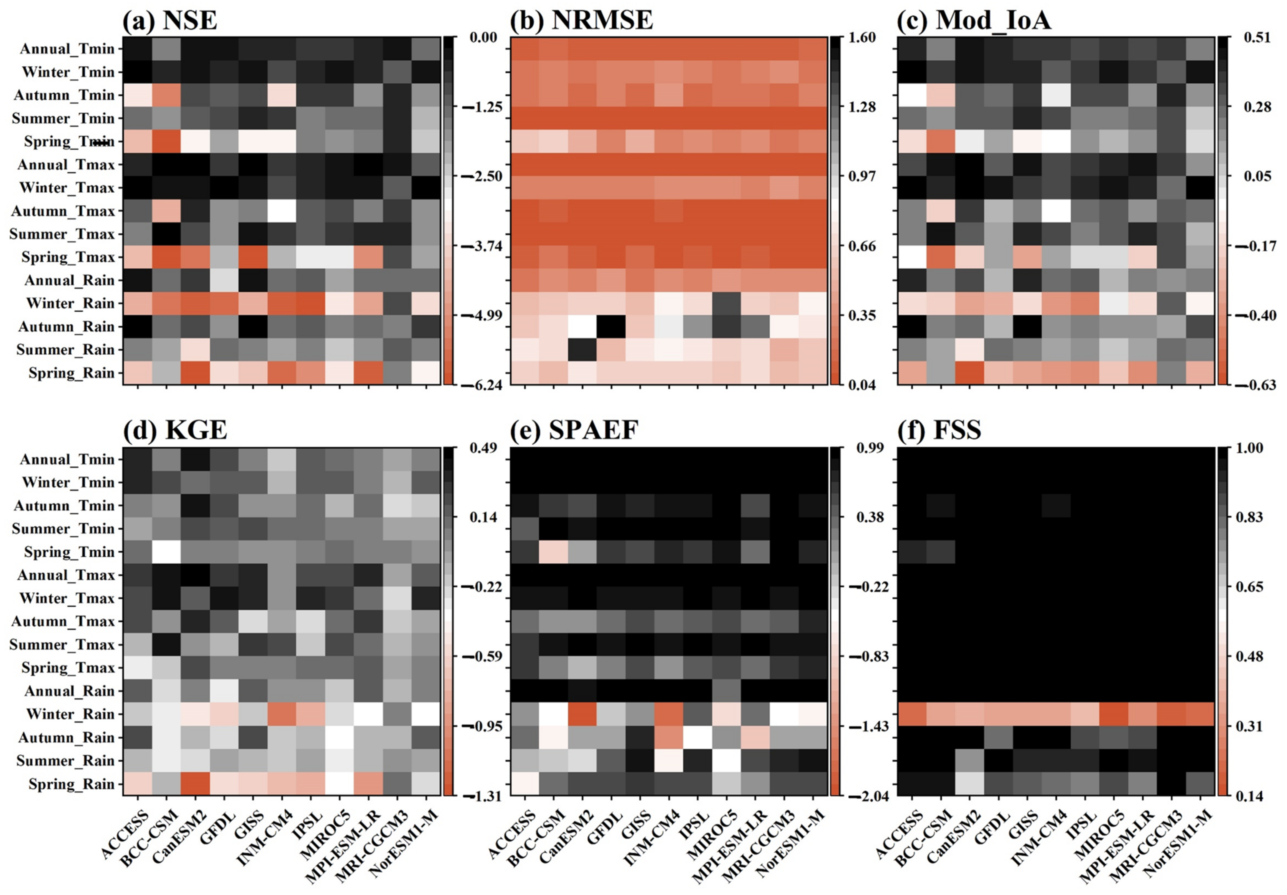
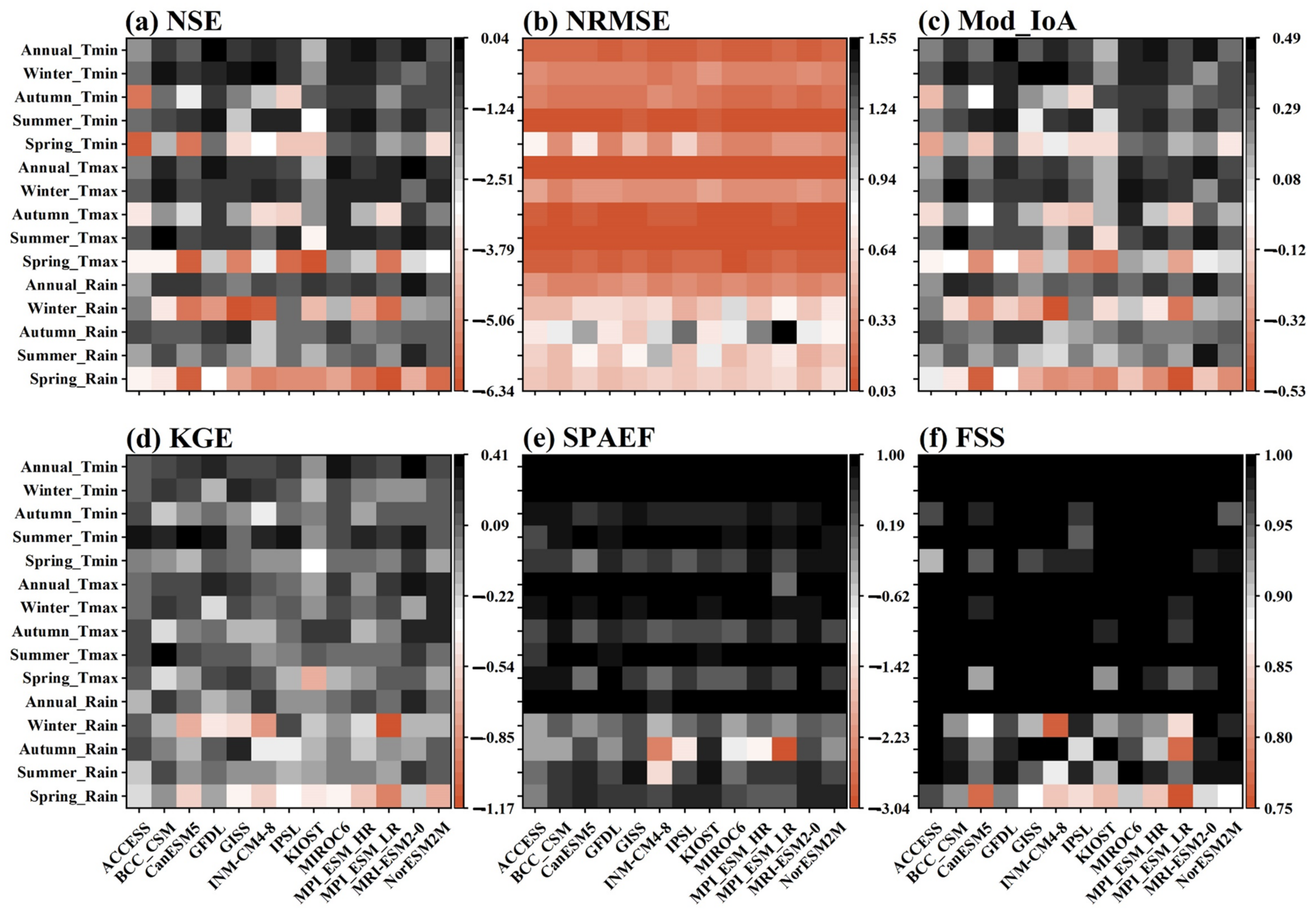
3.1.1. Performance Evaluation of GCMs

The performance evaluation of 24 GCMs, comprising 11 CMIP5 and 13 CMIP6 during the historical period (1975–2005) for the Chungcheong region of South Korea, was conducted based on three pairs of temporal and spatial indices. The results generally show that CMIP6 models moderately perform better than CMIP5 models in simulating historical rain, Tmax, and Tmin, especially in terms of NSE, NRMSE, Mod_IoA for temporal assessment and FSS and SPAEF for spatial assessment, where the majority of the models showed good performance for simulating a larger number of climate conditions on the seasonal and annual scales (Figure 2 and Figure 3). In the spring, the results indicate that MRI-CGCM3 from the CMIP5 is the best-performing model in simulating rain, Tmax, and Tmin, as shown by the majority of the indices such as NRMSE (0.51, 0.06, and 0.22), SPAEF (0.58, 0.63, and 0.92), and FSS (0.99, 0.99, 0.99), respectively (Figure 2). Although NSE values (<0.00) indicate poor performance for all the models including MRI-CGCM3, the majority of the models indicate poor performances in terms of other temporal and spatial assessments for the spring season, with CanESM2 being the worst-performing model considering all the climate conditions. For CMIP6 (Figure 3), GFDL is the best-performing model for rain, Tmax, and Tmin, especially in terms of NRMSE (0.49, 0.09, and 0.25), SPAEF (0.51, 0.90, and 0.64), and FSS (0.93, 0.99, and 0.99), respectively. However, similar to CMIP5 models, all CMIP6 models have NSE values lower than 0.00 and Mod_IoA and KGE values lower than 0.50 for the spring season.
In the summer, MRI-CGCM3 is the best-performing model from CMIP5 in simulating rain, Tmax, and Tmin when considering most indices. While other models indicate poor average values for many of the evaluating indices, the average values of NRMSE (0.47, 0.04, and 0.05), SPAEF (0.74, 0.87, and 0.93), and FSS (0.99, 0.99, and 0.99) indicate the reasonable performance of MRI-CGCM3 in simulating historical summer rain, Tmax, and Tmin, respectively. For CMIP6, MRI-ESM2-0 is the best-performing model in simulating historical summer rain, Tmax, and Tmin, as indicated by the majority of the indices, including NRMSE (0.45, 0.04, and 0.05), Mod_IoA (0.44, 0.43, and 0.39), SPAEF (0.63, 0.91, and 0.90), and FSS (0.99, 0.99, and 0.99), respectively. Generally, most models from CMIP5 and CMIP6 performed better in simulating Tmax and Tmin than rain. This can be attested to by their NRMSE (>0.5), SPAEF (−1.39 to 0.86), and FSS (0.89 to 0.99) for rain with corresponding values of <0.07, 0.51–0.93, and 0.98–0.99 for Tmax and <0.07, 0.40–0.96, 0.99 for Tmin, respectively.
There is a contrasting capability of model performance on precipitation and temperature in the autumn, especially for CMIP5. While ACCESS1-3 from CMIP5 performs better in simulating rain (NRMSE = 0.57, Mod_IoA = 0.47, FSS = 0.99), it performs poorly for both Tmax and Tmin based on most indices’ outputs. However, CanESM2 performs better for both Tmax and Tmin, as indicated by the NRMSE (0.06, 0.18), Mod_IoA (0.37, 0.29), and FSS (0.99, 0.99) values, respectively. For CMIP6, GFDL is the best-performing model in simulating rain, Tmax, and Tmin when considering most indices. Compared to CMIP5, ACCESS1-3 also performs relatively well for rain in CMIP6; however, CanESM2 performs poorly for Tmax, Tmin, and rain.
In the spring, similar to the summer season, MRI-CGCM3 is the most reasonably performing model from CMIP5 in jointly simulating the rain, Tmax, and Tmin from 1975 to 2005, as indicated by NRMSE (0.51, 0.06, and 0.22), SPAEF (0.58, 0.63, and 0.92), and FSS (0.99, 0.99, and 0.99), respectively. However, for CMIP6, GFDL is the best-performing model in simulating historical spring rain, Tmax, and Tmin, as indicated by the majority of the indices, including NRMSE (0.49, 0.09, and 0.25), SPAEF (0.51, 0.90, and 0.64), and FSS (0.93, 0.99, and 0.99), respectively. Although both MRI-CGCM3 and GFDL are considered as best-performing models for CMIP5 and CMIP6, respectively, the average values of indices such as NSE (<0.00), Mod_IoA (<0.50), KGE (0.20), however, indicate poor performances of these models.
Lastly, for the annual scale, ACCESS1-3 from CMIP5 is the best-performing model from CMIP5, as shown by most indicators, in simulating the historical rain, Tmax, and Tmin. For instance, the NRMSE (0.24, 0.05, and 0.12), Mod_IoA (0.41, 0.35, 0.43), SPAEF (0.93, 0.97, and 0.99), and FSS (0.99, 0.99, 0.99) values indicate average values for each of the performing indices in simulating rain, Tmax, and Tmin, respectively. The observed metric values are indications that ACCESS1-3 performs better in jointly simulating the three important variables of climate change in the Chungcheong region than other models in CMIP5. However, indices such as NSE and KGE did not show satisfactory results, not only for ACCESS1-3 but all the models. For CMIP6, MRI-ESM2-0 performs better according to the NRMSE (0.24, 0.04, 0.11), Mod_IoA (0.43, 0.45, 0.44), KGE (0.29, 0.35, 0.39), SPAEF (0.91, 0.99, 0.99), and FSS (0.99, 0.99, 0.99) indices, in simulating historical rain, Tmax, and Tmin, respectively. However, based on the relatively high average values of NRMSE and low values of the other indices, the model with poor performance in simulating historical variables of interest on the annual scale is ACCESS from CMIP6.

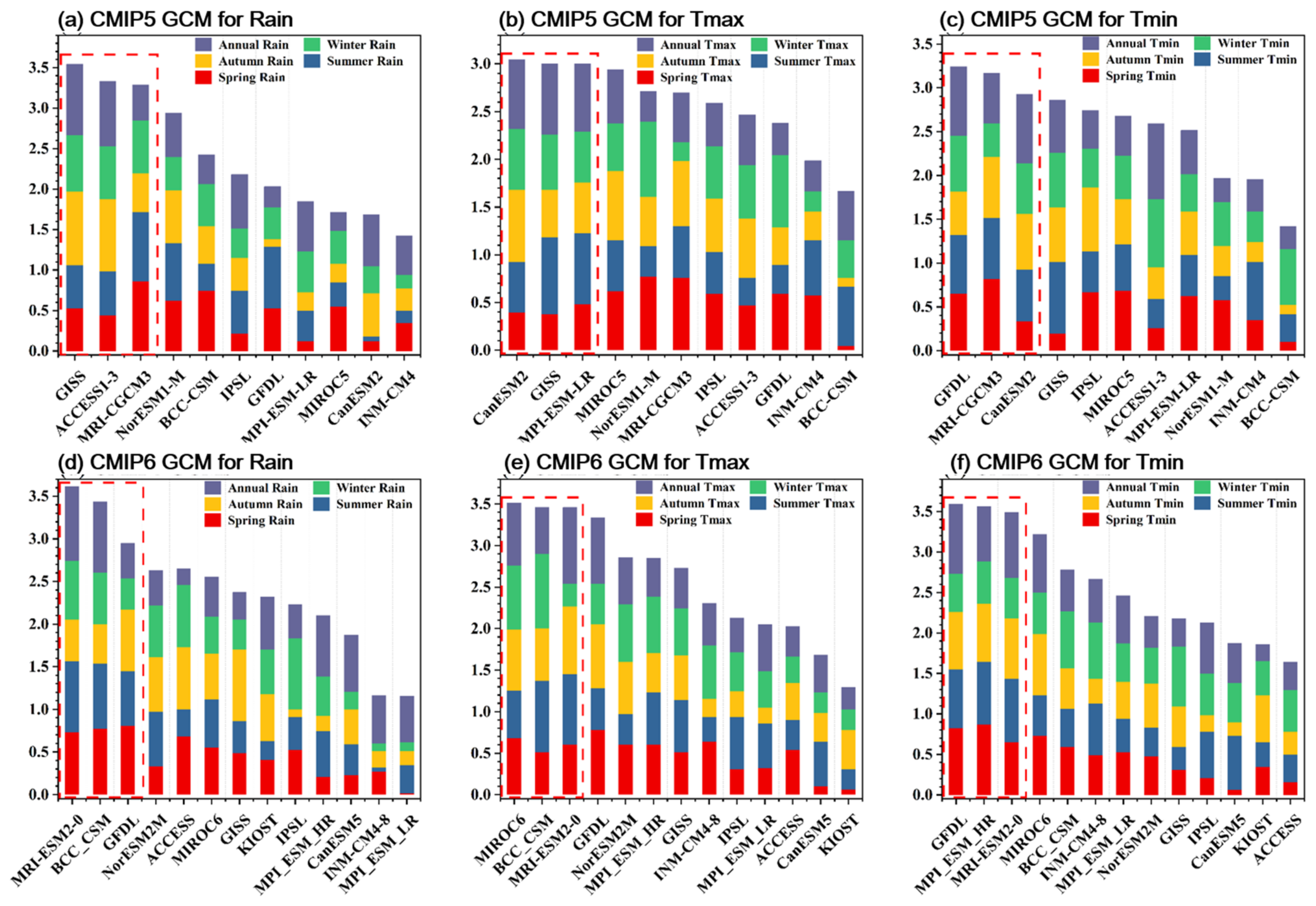
3.1.2. Comprehensive Ranking of CMIP5 and CMIP6 GCMs

Considering the different outputs obtained from the multiple metrics used in the performance evaluation of the GCMs, a comprehensive ranking was carried out by taking all six metrics and multiple climate conditions of seasonal and annual scales into account to obtain an overall ranking metric (Figure 4). As clearly observed in Figure 4a, GISS, ACCESS1-3, and MRI-CGCM3 are the top three ranked GCMs in simulating both the temporal and spatial characteristics of rain among the CMIP5 models. However, the poorest models for simulating rain based on the comprehensive ranking are MIROC5, CanESM2, and INM-CM4. Although some of the models are poorly ranked in terms of the cumulative ranking assessment, it can be observed that some models, such as GFDL and MIROC5, have relatively better performance rankings in reproducing selected climate conditions than the top-ranking models. For the CMIP6 GCMs, the top-ranking models are MRI-ESM2-0, BCC_CSM, and GFDL, while the poor-ranked models in simulating the rain based on temporal and spatial characteristics are CanESM5, INM-CM4-8, and MPI_ESM_LR (Figure 4d). Nevertheless, GISS and IPSL showed comparatively better performance rankings for reproducing autumn precipitation and winter precipitation, respectively.
Similarly, for reproducing the seasonal and annual Tmax using the CMIP5 GCMs, about eight out of the eleven models indicate better performance rankings (above 2.5) with CanESM2, GISS, and MPI-ESM-LR as the top three ranked models (Figure 4b). However, the NorESM1-M and MRI-CGCM3 models have higher rankings in simulating the temporal and spatial characteristics of spring Tmax than those obtained in the top three ranked models. For the CMIP6 models, only seven out of the thirteen models show good performance rankings of above 2.5, with MIROC6, BCC_CSM, and MRI-ESM2-0 being the top three ranked models (Figure 4e).
Further, in the CMIP5 GCMs, eight models are ranked above 2.5, while the top three ranking models for simulating the temporal and spatial characteristics of Tmin are GFDL, MRI-CGCM3, and CanESM2 (Figure 4c). However, the lowest-ranked CMIP5 models are NorESM1-M, INM-CM4, and BCC-CSM with ranking values below 2.5. Moreover, ACCESS1-3 and GISS show better performance rankings in reproducing the winter and summer Tmin, respectively, than the top three ranked models. For CMIP6 GCMs, only a few models (six) are ranked above 2.5 out of the 13 models that could reproduce the temporal and spatial characteristics of Tmin. The top three ranking models among the models are GFDL, MPI_ESM_HR, and MRI-ESM2-0, while the lowest ranked models are CanESM5, KIOST, and ACCESS (Figure 4c).

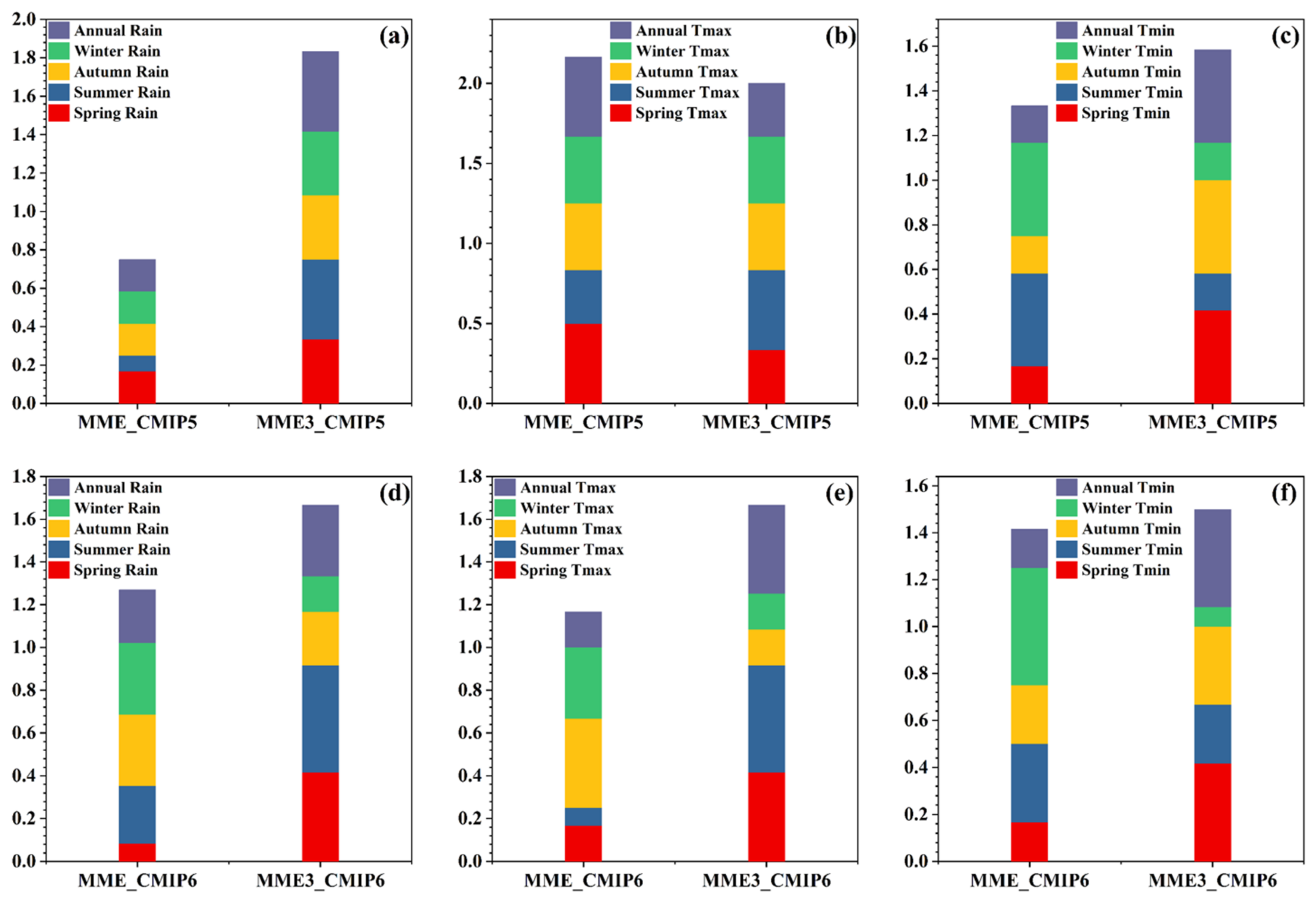
3.2. Selection of Multi-Model Ensemble Members

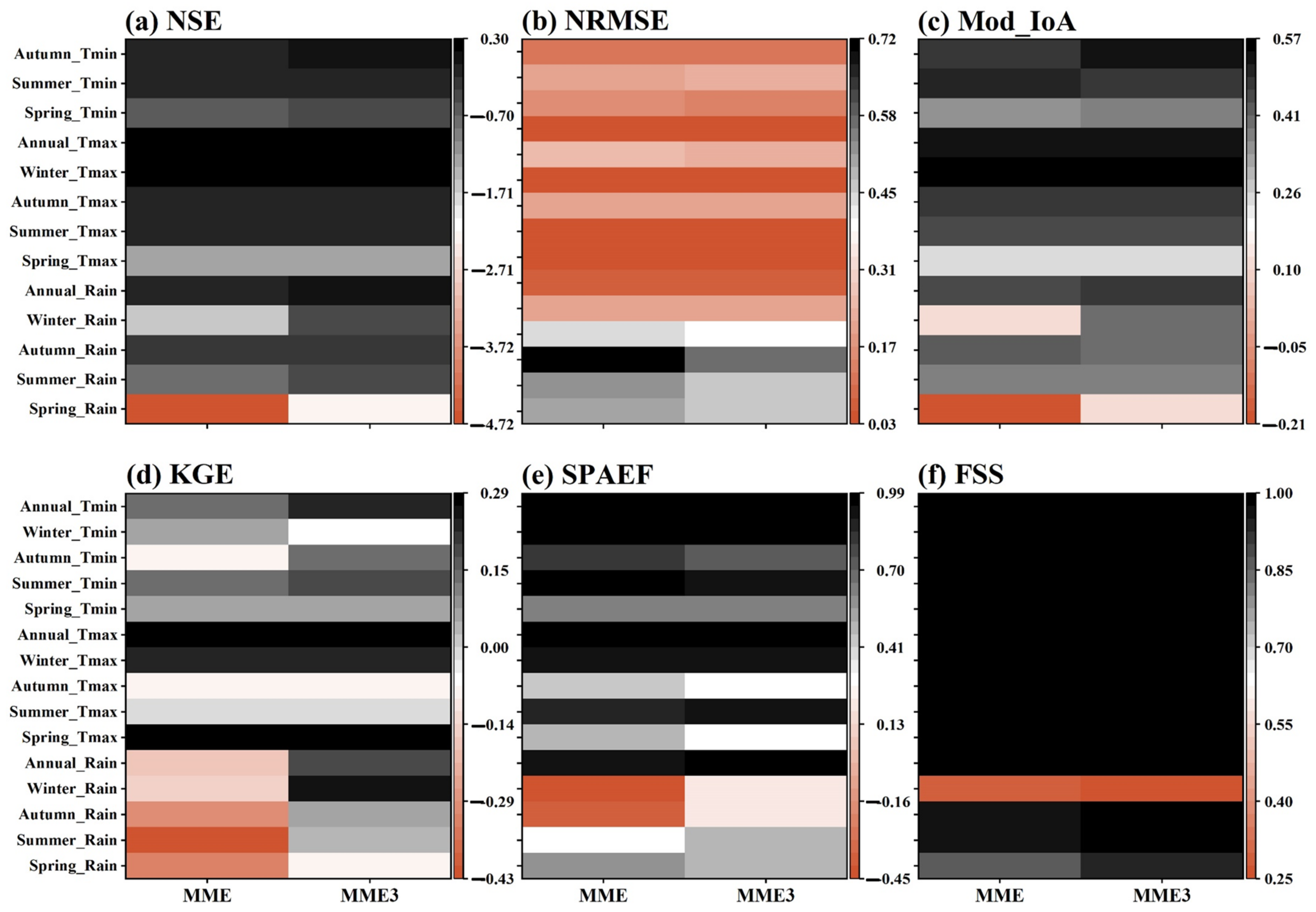
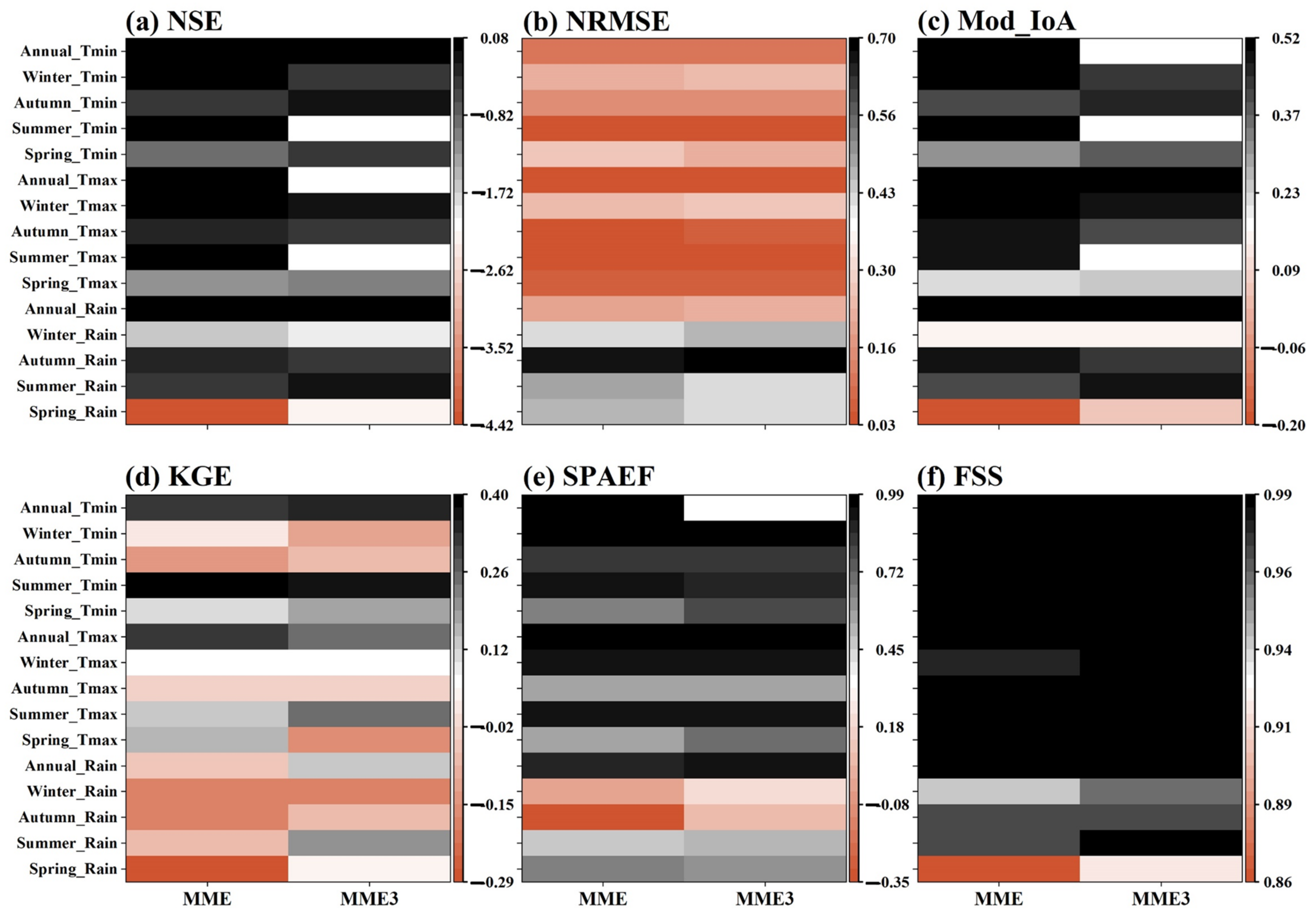
Performance of the Multi-Model Ensembles

The performance of the two developed multi-model ensembles in simulating the temporal and spatial characteristics of the climate variables under seasonal and annual scales was evaluated. The results show a distinct performance difference between the average of all the GCMs (MME) and the average of the top three GCMs (MME3) for both CMIP5 and CMIP6, as indicated by both temporal and spatial metrics (Figure 5 and Figure 6). For instance, in CMIP5, the average values of NRME range between 0.03 and 0.72 for MME, while the same metric ranges between 0.03 and 0.58 for MME3, indicating a better performance of MME3 in reproducing the temporal characteristics of rain, Tmax, and Tmin in the Chungcheong region of South Korea (Figure 5b). Similarly, the average values of SPAEF range between −0.45 and 0.99 for MME and between 0.20 and 0.99 for MME3, thus indicating a better performance of MME3 in simulating the spatial characteristics of rain, Tmax, and Tmin (Figure 5e).
For the CMIP6 GCMs, the visual representation of all six metrics in Figure 6 generally indicates the performance capability of MME3 over MME to reproduce the temporal characteristics of precipitation, Tmax, and Tmin in this study. However, there are a few selected climate conditions where MME performed better than the MME3. For instance, the average values of Mod_IoA for autumn and winter precipitation (0.48 and 0.50) in MME are higher than the average values of 0.42 and 0.42, respectively, indicating a better performance of MME over MME3 in simulating autumn and winter precipitation. Nevertheless, the general observation from most temporal and spatial metrics indicates the better performance of MME3 over MME in simulating seasonal and annual climate variables: rain, Tmax, and Tmin in the Chungcheong region of South Korea.
The results of the comprehensive ranking of the multi-model ensembles at seasonal and annual scales are shown in Figure 7. MME3 is ranked higher in all the climate conditions at seasonal and annual scales for both the CMIP5 and CMIP6 GCMs except for Tmax in CMIP5, where MME is ranked slightly higher than MME3 (Figure 7b). The high-performance rankings of spring Tmax and annual Tmax in MME influence the cumulative ranking over MME3, where the same climate conditions are ranked lower.
Similarly, despite the higher ranking of MME3 over MME from the cumulative comprehensive ranking results, the ranking by individual climate conditions shows that winter Tmin and annual Tmin have a higher ranking in MME than in MME3 for CMIP5. In contrast, winter and autumn precipitation, winter and autumn Tmax, and winter and summer Tmin ranked higher under MME than MME3. These results align with a study conducted by Ahmed et al., where it was observed that MME estimated from the best-performing GCMs had fewer uncertainties and performed better than results from individual GCMs [35].

3.3. Analysis of Future Precipitation and Temperature Changes

Understanding the future trends in rainfall and temperature is critical to prevent climate change-related impacts in an area. The seasonal and annual spatial changes in the average precipitation and temperature under four scenarios of RCPs and SSPs for future periods are compared to the baseline (Figure 8).

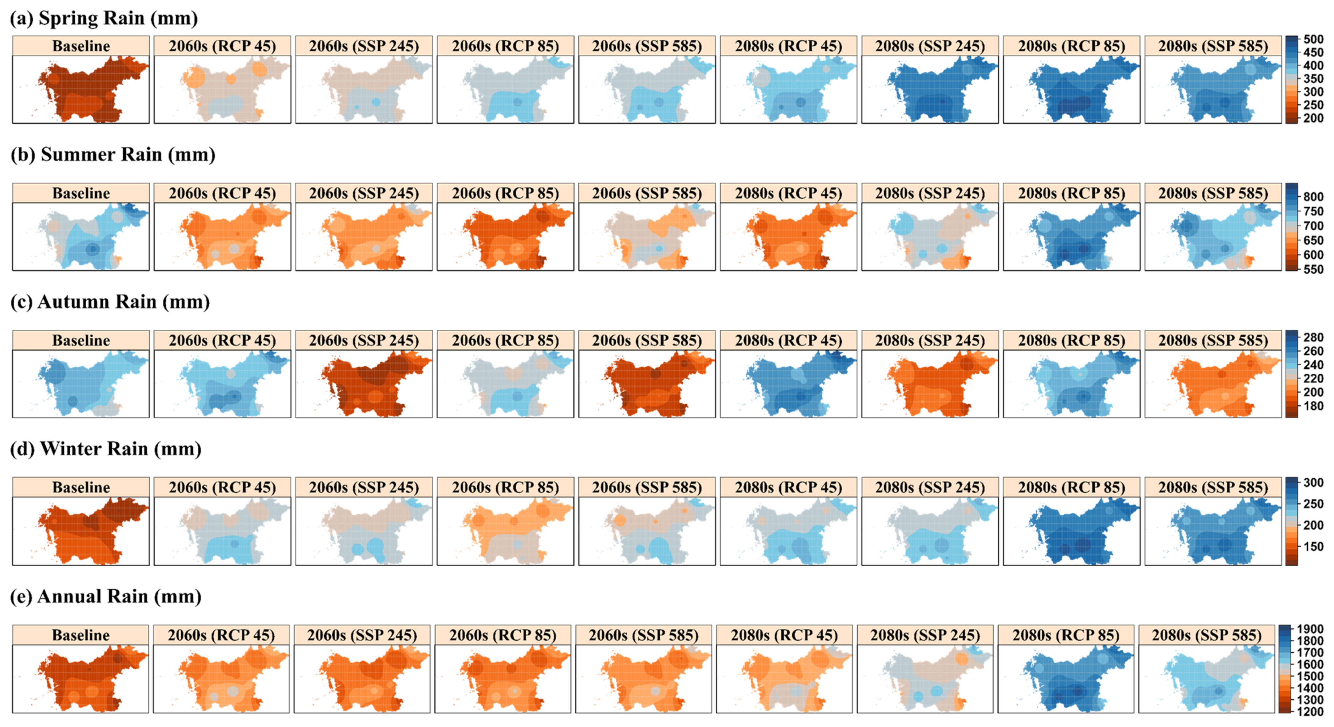
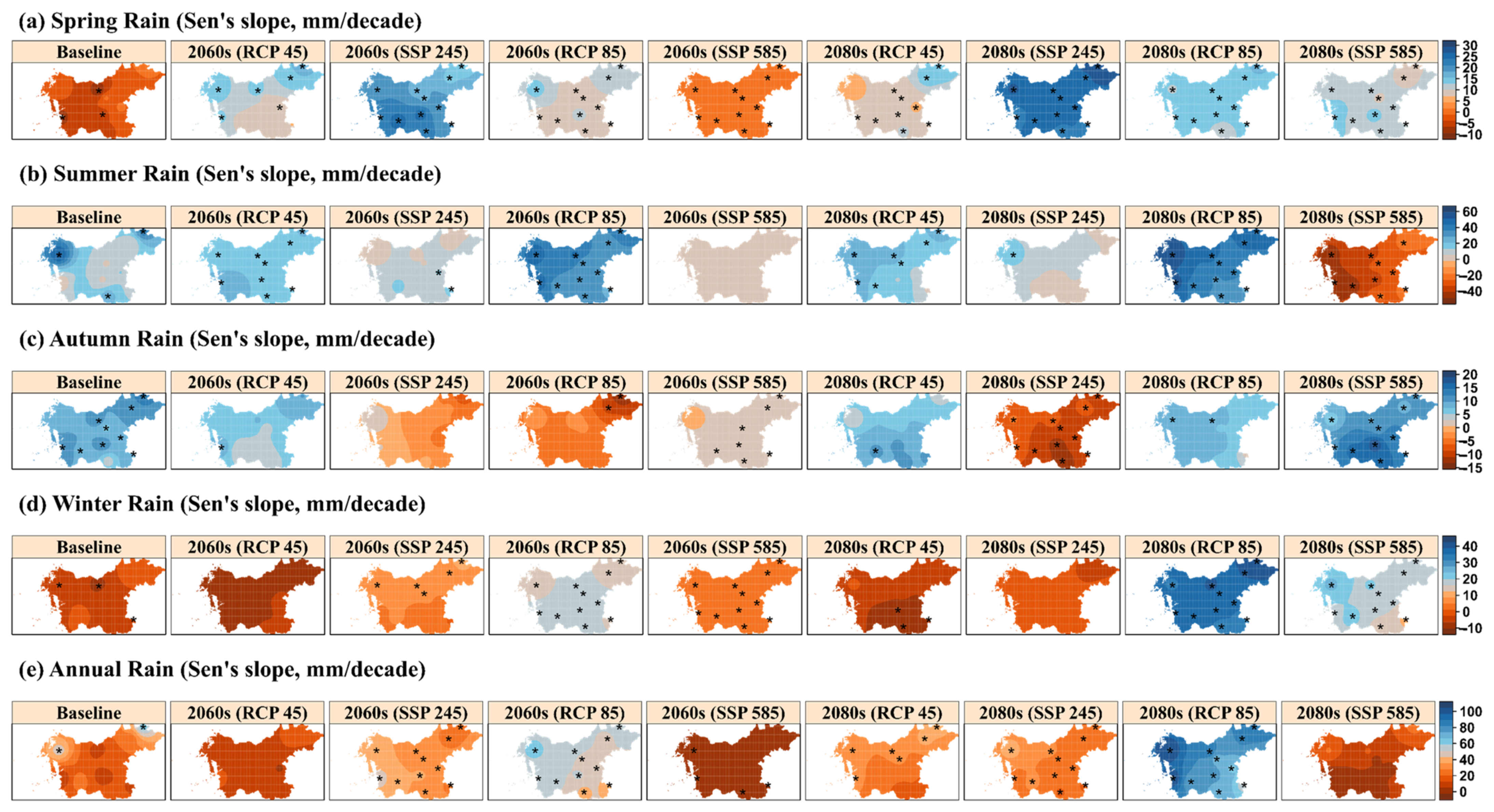
3.3.1. Spatial–Temporal Analysis and Trends in Seasonal and Annual Precipitation

The spatial patterns indicate varying differences in the rainfall distribution among the four scenarios, with the summer and autumn seasons showing significant differences, especially between RCPs and SSPs. The average changes in rainfall during the spring and winter seasons for both the near and far future, i.e., the 2060s (2021–2060) and 2080s (2061–2100), respectively, are expected to increase progressively for all RCPs except for winter precipitation, which shows a decrease under RCP8.5 in the near future. For SSPs, on the other hand, the summer precipitation increases progressively after showing a significant decrease during the 2060s. However, it continuously decreases under RCPs until the 2080s, when it increases significantly.
The precipitation distribution at both seasonal and annual scales exhibit increasing trends toward the southern part of the Chungcheong region, with average values ranging from 744.95 mm to 827.66 mm for summer precipitation under RCP8.5 in the 2080s. However, autumn precipitation is expected to drastically decrease under SSP scenarios during both the 2060s and 2080s, with the lowest average precipitation of 170.33 mm occurring at the northern part under SSP2-4.5 in the near future. This is in contrast with the changes in the distribution patterns under RCPs, where autumn precipitation is expected to increase with a maximum average rainfall of 282.09 mm in the northeast end under RCP4.5 in the far future.
For the average annual precipitation, the spatial distribution shows a slight increase in annual average rainfall with similar patterns for both RCP and SSP scenarios during the near future periods. Specifically, the maximum average amount of precipitation during the period of the 2060s increases from 1417.56 mm (historical) to 1557.49 mm (RCP4.5), 1570.54 mm (SSP2-4.5), 1520.28 mm (RCP 85), and 1885.55 mm (SSP585), respectively. Meanwhile, there is an apparent increasing trend from the north to the southern part under the four considered scenarios in the periods of the 2060s and 2080s.
Overall, the maximum annual average precipitation of 1885.55 mm is expected to occur during the far future under the RCP8.5 scenario, while the SSP5-8.5 scenario during the same period indicated lower annual average maximum precipitation (1728.79 mm). Furthermore, the variability in the precipitation distribution in the entire Chungcheong region is low under RCP8.5 compared with SSP5-8.5 during the 2080s.
To further understand the changes in spatial patterns of precipitation distribution during the near and far future as compared with the historical periods under the RCP and SSP scenarios, a trend analysis was performed using the MMK test with a statistical significance of trends at p ≤ 0.05, while the trend magnitude was estimated using Sen’s slope. For instance, the temporal trends in spring, winter, and annual precipitation (Figure 9a,d,e) during the historical periods show decreasing trends, which are predominantly nonsignificant; however, summer and autumn precipitation exhibit sparsely and predominantly increasing trends, respectively.
The results of trends in precipitation changes indicate a high level of inconsistency under different scenarios and during different periods. For both near and far future periods under RCP scenarios, the precipitation in spring and summer (Figure 9a,b) exhibits significantly increasing change rates compared with their historical trends with maximum change rates of 29.38 mm/decade and 59.39 mm/decade, respectively, observed during the 2080s period. In autumn (Figure 9c), precipitation is expected to change moderately and at sparingly significant locations for the majority of the RCP scenarios except for the period of 2060s under RCP8.5, where a rapid and significant decreasing trend of −13.23 mm/decade at the northeast end of the Chungcheong region is expected to occur. Meanwhile, the winter and annual precipitation (Figure 9d,e) show rapid and statistically significant change rates with average values of 42.57 mm/decade and 1885.55 mm/decade, respectively, under RCP8.5 during the 2080s compared with the observed maximum values of 1.09 mm/decade and 61.29 mm/decade for the historical period and 19.04 mm/decade and 61.02 mm/decade for the near future period, respectively, under different scenarios.
The irregularity in the trend pattern of precipitation is more demonstrated under the SSP scenarios. In spring, while the maximum significant increasing rate of rainfall is 25.67 mm/decade in the near future periods under SSP2-4.5, the SSP5-8.5 scenario exhibits a significant decreasing trend with an average value of 1.22 mm/decade (Figure 9a). Overall, the maximum significant change rate of 29.38 mm/decade for spring rain occurs under the SSP2-4.5 scenario in the 2080s. For summer rain, the SSP scenarios in the 2060s and 2080s exhibit decreasing trends, which become predominantly significant with intense magnitude (−48.63 mm/decade on average) under SSP5-8.5 during the far future period. Similarly, autumn precipitation under SSP2-4.5 and 585 in the 2060s and SSP2-4.5 in the 2080s exhibit consistent decreasing trends, which become significant mainly with a maximum average change rate of −12.36 mm/decade under SSP2-4.5 in the far future period. However, significantly increasing trends are expected to occur under the SSP5-8.5 scenario in the far future, with an average change rate of 19.00 mm/decade.
Further, winter rain exhibits a moderate change rate under SSP scenarios in the 2060s and 2080s except for SSP5-8.5 during the 2080s, which shows an improved significantly increasing trends at an average rate of 24.51 mm around the western part, where the change is maximum. Lastly, the change rate of annual rain moderately increases with statistical significance under the SSP2-4.5 scenario to maximum values of 46.73 mm and 39.18 mm around the western part in the near and far future periods, respectively. However, the decreasing trends with sparing significance under SSP5-8.5 during the 2060s but no significance under SSP5-8.5 during the 2080s are exhibited for annual rain.

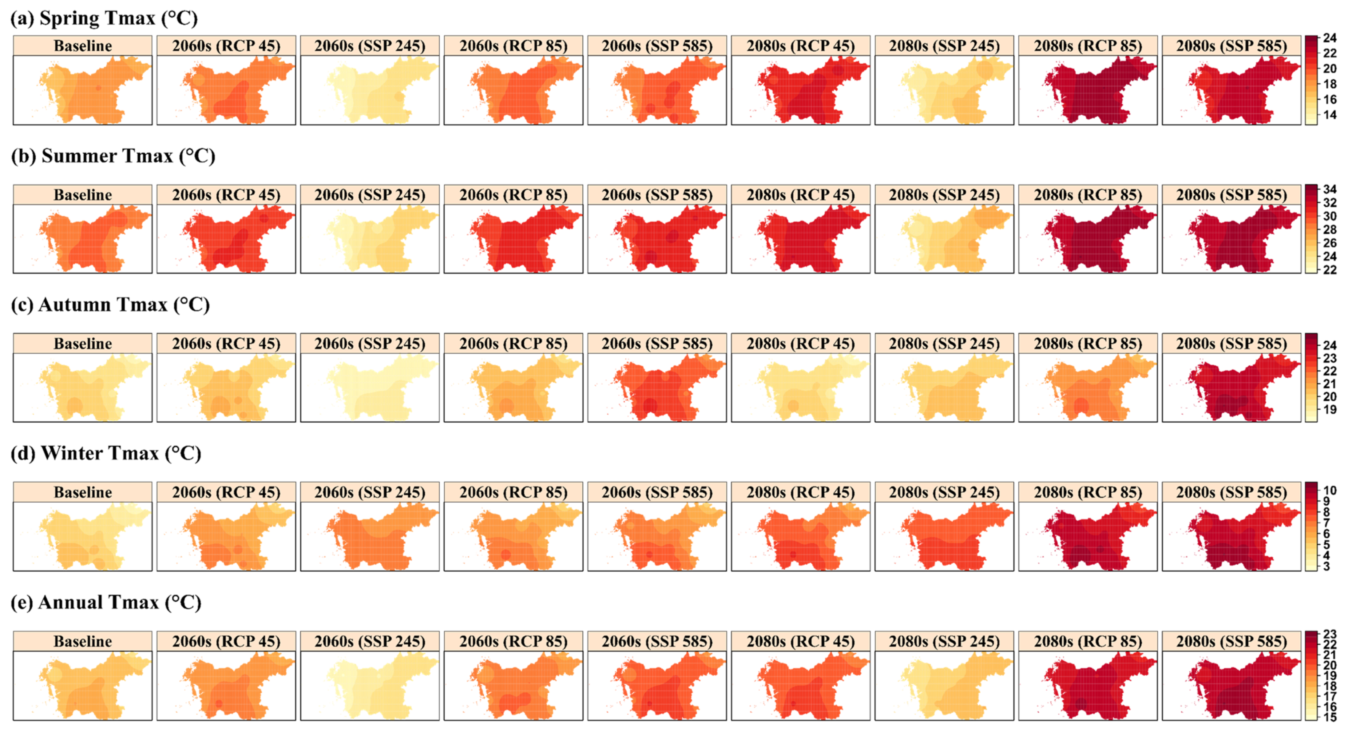
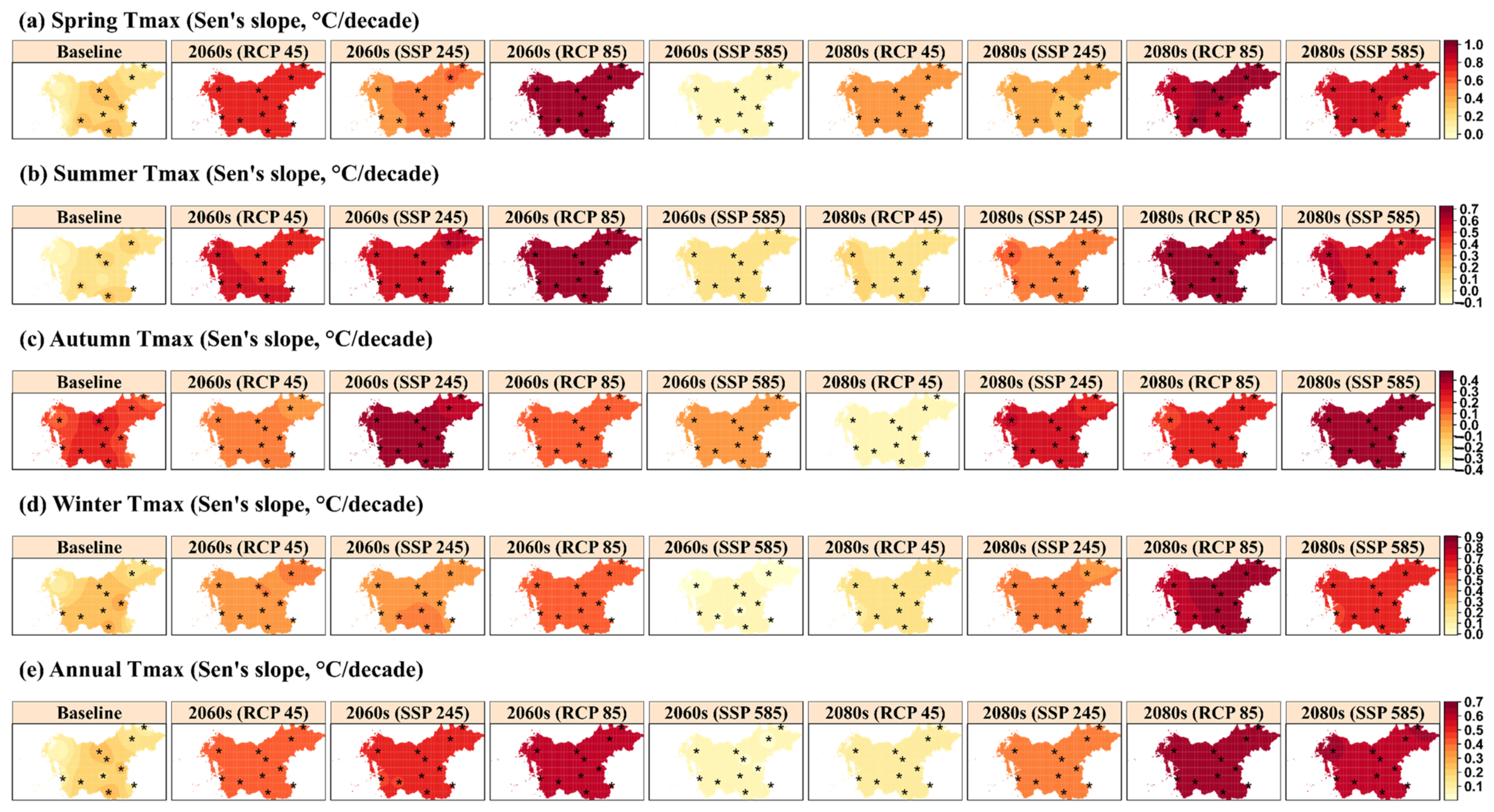
3.3.2. Spatial–Temporal Trends in Seasonal and Annual Tmax

The spatial distributions of seasonal and annual average Tmax during the historical and future periods under the RCP and SSP scenarios across the Chungcheong region are shown in Figure 10. The results show that the Tmax consistently increases from the historical period to the near and far future periods under the RCP4.5 and RCP8.5 scenarios for the four seasons and at the annual scale. The expected increment in the average Tmax in all the seasons and at the annual scale is expected during the 2080s and under RCP8.5 and SSP5-8.5. Summer is the hottest season in South Korea; the average Tmax is likely to increase up to 33.84 °C in the southern part of the region under RCP 80 in the 2080s, while the highest value under SSP5-8.5 in the same far-future periods is 33.59 °C, which extends from the north to the central and the southern part of the region (Figure 10b). The summer temperature increase covers over 80% of the entire Chungcheong region. However, Tmax is expected to decrease during the near and far future periods with maximum values of 25.51 °C and 26.72 °C, respectively, around the northeast part under the SSP2-4.5 scenario.
The highest occurring value of Tmax in the spring is 23.54 °C under RCP8.5 in the 2080s, while it decreases under SSP2-4.5 in the 2060s and 2080s to maximum values of 15.71 °C and 16.68 °C, respectively (Figure 10a). There is a moderate to high increase in the average Tmax from the 2060s to 2080s under RCP4.5. The distribution patterns of the highest and lowest occurring Tmax in spring are similar to the observations in the summer under the same RCP8.5 and SSP2-4.5 scenarios in the 2080s and 2060s, respectively. In autumn, however, the significant increase in Tmax only occurs under SSP5-8.5 scenarios during both the near and far future with values of 23.05 °C and 24.50 °C, respectively (Figure 10c). Similar to other seasons and annual averages, the lowest Tmax with a maximum value of 19.18 °C occurs in the 2060s under the SSP2-4.5 scenario.
Tmax in the winter progressively increases from the near future period to the far future period, with the RCP and SSP scenarios showing the same incremental patterns. While the highest values of Tmax expected to occur under the RCP and SSP scenarios are 10.13 °C and 10.25 °C in the 2080s, respectively, which progressively increase from the north down to the southern part, and the lowest values are 4.60 °C and 5.06 °C under RCP and SSP scenarios in the 2060s (Figure 10d). Meanwhile, there are contrasting distributions of annual Tmax under RCP4.5 and SSP2-4.5, such that Tmax is expected to increase to 19.61 °C and 20.63 °C under RCP4.5 in the near and far future periods, respectively (Figure 10e). However, Tmax is likely to decrease with maximum values of 16.78 °C and 17.91 °C under SSP2-4.5 in the near and far future, respectively. Overall, the highest annual average Tmax of 22.41 °C and 22.73 °C are expected to occur during the distant future period under RCP8.5 and SSP5-8.5, respectively.
As shown in Figure 11, the seasonal and annual Tmax trends indicate significant statistical changes during the historical and future periods of both near (2060s) and far (2080s) under the RCP and SSP scenarios. In the spring, the maximum changes in Tmax occur under the RCP8.5 scenario in the 2060s at a significant rate of 0.72–0.77 °C/decade (Figure 11a), which is also the maximum expected change in Tmax in both the near and far future under all RCP and SSP scenarios across seasons and the annual scale (Figure 11). However, the lowest changes in spring Tmax occur during the 2060s under SSPs 585 at a significant rate of 0.06 °C/decade. The rate of change significantly decreases from the near to the far future under RCP4.5, RCP8.5, and SSP2-4.5 at an average of 0.75 to 0.45 °C/decade, 0.94 to 0.91 °C/decade, and 0.52 to 0.37 °C/decade, respectively, while only under SSP5-8.5 is an increase in Tmax expected from the 2060s to 2080s at an average rate of 0.06 °C/decade to 0.78 °C/decade, respectively.
In the summer, the maximum increasing changes in Tmax occur in the 2060s under the RCP8.5 scenario at an average rate of 0.67 °C/decade, while a significantly decreasing trend at an average rate of 0.05 °C/decade and 0.09 °C/decade occur under SSP5-8.5 and RCP4.5 during the 2060s and 2080s, respectively (Figure 11b). However, there is a moderate decreasing trend in the 2080s, especially around the northeast area at 0.60 °C/decade. The decreasing trends from west to east-northward occurred under RCP4.5 and SSP5-8.5 in the 2060s and 2080s, respectively. In the autumn, on the other hand, Tmax has a maximum increasing trends at an average rate of 0.41 °C/decade under SSP5-8.5 in the 2080s (Figure 11c). Although there is a decreasing trend from the 2060s to 2080s under SSP 24, both periods have a similar pattern in the change rate such that the trend decreases toward the northeast end. Further, a maximum significant decreasing trend occurred in the 2080s under the RCP4.5 scenario at the rate of −0.34 °C/decade. For the winter season, there are moderate to high increasing trends from the 2060s to 2080s under the SSP2-4.5 and RCP8.5 scenarios, respectively, while significant decreasing trends occur in the 2060s and 2080s under SSP5-8.5 and RCP4.5, respectively (Figure 11d). The average maximum increasing trend is 0.81 °C/decade, occurring from the west to the northeastern part. The average maximum decreasing trend is 0.05 °C/decade under the SSP5-8.5 scenario in the 2060s. The annual Tmax follows similar trend patterns in summer Tmax, such that the maximum increasing trends occur under RCP8.5 in the 2080s at an average rate of 0.64 °C/decade, while the maximum decreasing trend of 0.05 °C/decade occurs in the 2060s under SSP5-8.5 scenarios (Figure 11e). Further, similar to the spring season, the rate of change significantly decreases from the near to the far future under RCP4.5 and SSP2-4.5 at an average of 0.43 to 0.09 °C/decade and 0.49 to 0.36 °C/decade, respectively. However, RCP8.5 and SSP5-8.5 moderately and intensely increase at average rates of 0.58 to 0.64 °C/decade and 0.05 to 0.61 °C/decade from the near to the far future, respectively.

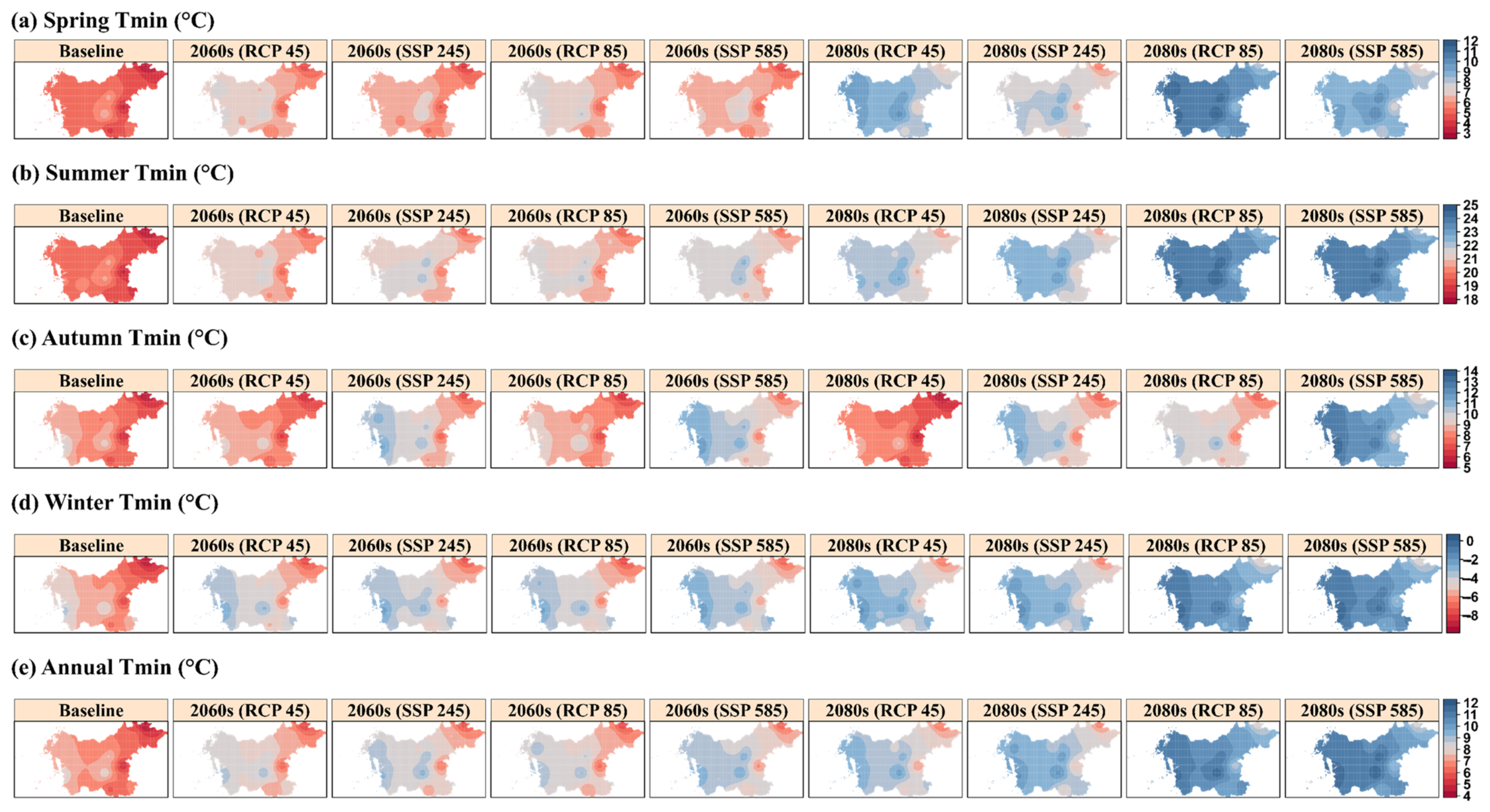
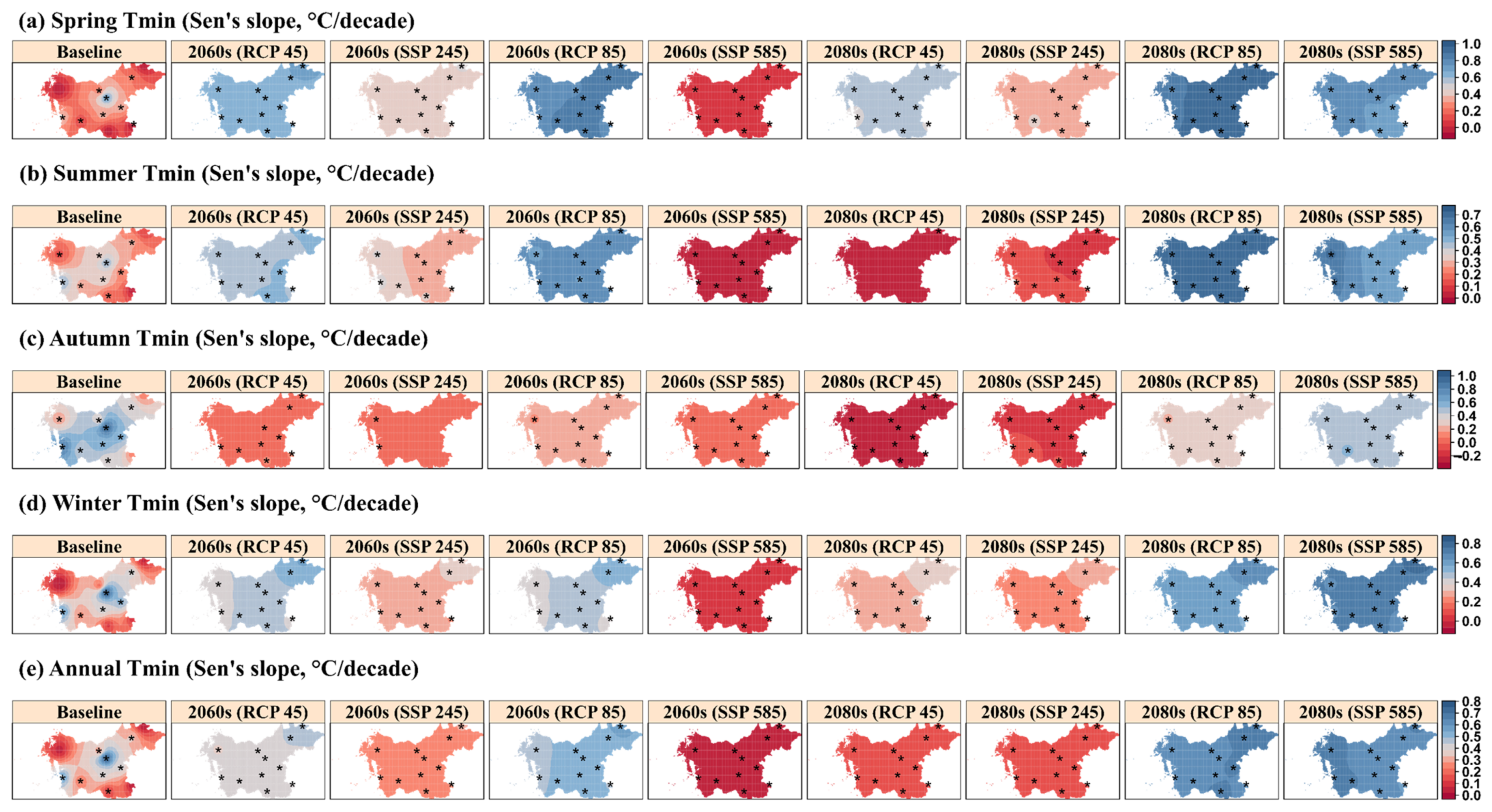
3.3.3. Spatial–Temporal Trends in Seasonal and Annual Tmin

Figure 12 shows the spatial patterns in historical and projected changes in seasonal and annual average Tmin during the near and far future under the RCP and SSP scenarios. It can be clearly observed that Tmin increases consistently from the historical period to the near and far future under the four considered scenarios of RCPs and SSPs in the four seasons and the annual scale; however, it varies in intensities. In the spring, the maximum Tmin is 10.25 °C under the SSP5-8.5 scenario in the 2080s, which occurs around the western part of the Chungcheong region (Figure 12a). Nonetheless, the lowest Tmin (4.17 °C) appears around the northeast under the SSP2-4.5 scenario in the near future. While there is a high increase in the average Tmin from the 2060s to 2080s under RCP4.5, RCP 85, and SSP5-8.5, especially from the west to the central part, only a moderate increase is observed under SSP2-4.5. In the summer, the average Tmin is expected to reach up to 24.57 °C and 24.46 °C in the central region under the RCP8.5 and SSP5-8.5 scenarios, respectively, in the 2080s. In comparison, there are low distribution patterns in Tmin during the 2060s, which decreases from the west toward the east, with the lowest average value of 19.48 °C under the RCP4.5 scenario (Figure 12b).
In the autumn, the distribution of Tmin follows similar patterns across the seasons and annually and for different scenarios, such that Tmin increases from the northeast end to the west region (Figure 12c). While a maximum Tmin of 13.57 °C occurs around the west area under SSP5-8.5 in the 2080s, the minimum Tmin is 5.53 °C and occurs at the northeast end under RCP4.5 in the 2080s. Winter is expected to progressively increase in Tmin during the near and future periods under the RCP and SSP scenarios (Figure 12d). However, the northeast region shows a low to moderate increase for all RCP and SSP scenarios in the 2060s and 2080s, except for RCP8.5 and SSP5-8.5, which show a considerable increase in Tmin. The average Tmin reaches up to −0.19 °C and 0.05 °C in the west region under the RCP8.5 and SSP5-8.5 scenarios, respectively, in the 2080s, while the lowest Tmin is −7.72 °C, which occurs around the northeast end under RCP4.5 in the 2060s (Figure 12d). Lastly, the annual Tmin also has a progressive distribution pattern, such that under RCP4.5 and SSP2-4.5, the average Tmin moderately increases from 7.70 and 8.01 °C in the 2060s to 8.55 and 8.99 °C in the 2080s, respectively (Figure 12e). However, under RCP8.5 and SSP5-8.5, it intensely increases from 7.85 and 8.34 °C in the 2060s to 10.30 and 10.53 °C in the 2080s, respectively.
As shown in Figure 13, the trends in seasonal and annual Tmin indicate statistically significant changes during the historical and future periods in both the near and far future under the RCP and SSP scenarios. In the spring, the trend in Tmin significantly increases at an average maximum rate of 0.91 °C/decade under the RCP8.5 scenario in the 2080s, while a decreasing trend rate of 0.05 °C/decade occurs under the SSP5-8.5 scenario in the 2060s (Figure 13a). While the trend moderately decreases under RCP4.5 and SSP2-4.5 from the 2060s and 2080s at an average of 0.65 to 0.54 °C/decade and 0.42 to 0.36 °C/decade, respectively, the trend significantly increases at an average rate of 0.05 to 0.75 °C/decade under SSP5-8.5 scenario in the near and far future, respectively.
In the summer, the trend rate decreases from west to east under SSP2-4.5 in both the 2060s and 2080s while increases from west to northeast under RCP4.5 and SSP5-8.5 in the 2060s and 2080s, respectively (Figure 13b). The maximum significant increasing trend rate occurs under RCP8.5 in the 2080s at 0.70 °C/decade, while maximum decreasing trends occur at a rate of 0.05 °C/decade and 0.02 °C/decade under SSP5-8.5 and RCP4.5 in the 2060s with RCP4.5 being sparingly significant at the northeast end (Figure 13b). In the autumn, the maximum increasing trend in Tmin occurs in the 2080s under the SSP5-8.5 scenario at an average rate of 0.51 °C/decade, while a significantly decreasing trend at an average rate of −0.29 °C/decade occurs under RCP4.5 in the 2080s (Figure 13c). The change rate in winter Tmin follows similar patterns under RCP4.5 and RCP8.5 in the 2060s, such that the trend rates progressively increase from the west to the central and the northeast end with distinct patterns, unlike other future scenarios where the trend rate increases only at the northeast end (Figure 13d). The rate of change significantly increases from the near to the far future under SSP5-8.5 at an average of 0.03 to 0.51 °C/decade, respectively. The average maximum increasing trend rate of 0.64 °C/decade occurs under RCP8.5 and around the northeast end in the 2080s, while a significantly decreasing trend at an average rate of 0.04 °C/decade occurs under SSP5-8.5 in the 2060s (Figure 13e). While the trend rate increases from the west toward the northeast end under RCP4.5 in the near future, the increase in trend is from the east toward the west under the SSP5-8.5 scenario in the 2080s at an average rate of 0.64 °C/decade.

4. Discussion

Generally, the models in CMIP6 show an improved performance in reproducing the temporal and spatial characteristics of rainfall, Tmax, and Tmin compared with CMIP5 in the Chungcheong region of South Korea. This can be primarily attributed to the improved spatial resolutions and enhanced climate sensitivity in CMIP6 [39]. Previous studies have also demonstrated the high performance of CMIP6 over CMIP5, especially in South Korea [3,40,41]. Cannon, 2020 [40] reported an improved simulation of historical monthly precipitation in CMIP6 models compared with CMIP5 models over South Korea based on selected indices, including a reduction in NRMSE (2.13%) and NSE (0.37%). This study used six evaluation indices, and the majority of these indices indicate the varying performance of individual GCMs on the reproducibility of temporal and spatial characteristics of climate variables. Although there is inter-model performance variability among the GCMs for each climate variable, the GISS, ACCESS1-3, MRI-CGCM3, CanESM2, MPI-ESM-L-R and GFDL models in CMIP5 are identified to perform better, while MRI-ESM2-0, BCC_CSM, MIROC6, MPI_ESM_HR, and GFDL are the better-performing models in CMIP6. Several studies have been conducted that also confirmed these models satisfactorily reproduce both temporal and spatial characteristics of climate variables in South Korea and East Asia in general, and these models have also been used to generate MME [15,20,42].
The multi-model ensembles derived from the top three performing models yielded better results in reproducing historical climate variables than those derived from the average of all the GCMs. This can be attributed to the reduction in the uncertainty associated with the GCMs when using suitable ensemble models [35,42]. Previous studies also reported similar superiority of multi-model ensembles over individual GCM [11,43]. Furthermore, the method used in the development of an MME could also influence the performance capability of the models. Hamed et al. found that the MME of the GCM ensemble, especially that which was derived from median rather than mean, performed better than a single GCM for climate projections [43]. Similar results were also reported by Ahmed et al., where MMEs based on random forest performed better than MMEs based on a simple mean using selected spatial performance metrics [35]. The differences in the results obtained from different MMEs indicate the need to consider the choice of GCMs and the appropriate method to generate MMEs that will perform better for a region of interest [12].
The future projection in CMIP5 and CMIP6 generally indicates an increase in average rain, Tmax, and Tmin; however, with distinct changes under similar radiative forcing levels in different periods over the Chungcheong region. The projections under RCPs 45 and 85 are expected to increase more than the SSP2-4.5 and 585 scenarios, which is more pronounced under RCP8.5 than SSP5-8.5 in the far future (2080s), especially for rain. The average summer rain change in the far future is projected to increase with respect to the historical period by 6.37% for RCP8.5 and 0.39% for SSP5-8.5, increase in spring rain by 107.38% for RCP8.5 and 95.53% for SSP5-8.5, increase in winter rain by 96.84% for RCP8.5 and 87.45% for SSP5-8.5, and increase in average rainfall by 31.75% for RCP8.5 and 21.89% for SSP5-8.5. Similarly, the average change in Tmax and Tmin increases in the summer by 15.63% and 20.96% for RCP8.5 and 14.81% and 20.16% for SSP5-8.5, increases in the spring by 29.00% and 112.03% for RCP8.5 and 23.91% and 83.34% for SSP5-8.5, and increases in the autumn by 9.03% and 19.90% for RCP8.5 and 20.82% and 48.75% for SSP5-8.5, and the average annual Tmax and Tmin increases by 22.61% and 58.72% for RCP8.5 and 24.35% and 62.16% for SSP5-8.5, respectively. It is worth noting that there are inconsistencies in some average changes in climate conditions of rain, Tmax, and Tmin between scenarios under similar radiative forcing levels such as RCP4.5 and SSP2-4.5 or RCP8.5 and SSP5-8.5 in different periods.
Many studies have also projected an increase in precipitation and temperature changes globally and in South Korea [11,42,44,45]. However, the extent of such increment could vary based on the region of interest and the type GCMs, as well as the assessment indices used [11,46]. The summer mean precipitation under all RCPs was projected to increase up to 15% using the BCC_CSM1.1 model in CMIP5 over East Asia [47], while Song et al. projected an increase in summer, winter, and annual precipitation by 19.7%, 47.4%, and 20.5% for RCP4.5 and by 18.9%, 15.9% and 24.6% for SSP5-8.5, respectively, using INM-CM4 from CMIP5 and INM-CM5 from CMIP6 [46]. In terms of temperature changes, it was reported that projected temperature will decrease in the near future but increase significantly in the far future with RCPs 4.5 and 8.5 by 9.1% and 17.6%, respectively, while SSPs 245 and 585 project increases of 6.9% and 19.1%, respectively [42]. The difference in these results could be attributed to selecting a single model from each CMIP5 and CMIP6 rather than the best-performing ensemble models used in the present study. However, a single model has been previously suggested against climate change projection due to its inability to provide uncertainty in climate projections [43]. At the same time, the present study used daily climate data, and the referenced studies used monthly climate data. Furthermore, both RCP and SSP scenarios are made up of different emissions pathways, including the composition of CO2 and non-CO2 [48]. The future changes in the mean precipitation associated with the East Asian summer monsoon are influenced by moisture flux changes and attributed to local climate conditions [49].

5. Conclusions

In this study, a performance evaluation of 24 GCMs comprising 11 and 13 models in CMIP5 and CMIP6, respectively, and their multi-model ensembles was carried out to assess the simulation capability of local climate characteristics over the Chungcheong region of South Korea from 1975 to 2015. The bias correction was first carried out using IDW and quantile mapping. Six performance indices comprising NSE, NRMSE, and Mod_IoA (temporal assessment) and KGE, SPAEF, and FSS (spatial assessments) were used to assess the reproducibility of the CMIP5 and CMIP6 GCMs and their generated multi-model ensembles. The trends in rain, Tmax, and Tmin under four scenarios of RCP and SSP were further analyzed for seasonal and annual scales in the near future: 2060s (2021–2060) and far future: 2080s (2061–2100).
The performance of CMIP6 models was relatively better in reproducing the temporal and spatial characteristics of historical climate variables based on the majority of the evaluating indices. The top three performing models in CMIP5 are GISS, ACCESS1-3, and MRI-CGCM3 for rain; CanESM2, GISS, and MPI-ESM-L-R for Tmax; and GFDL, MRI-CGCM3, and CanESM2 for Tmin. While the top three performing models in CMIP6 are MRI-ESM2-0, BCC_CSM, and GFDL for rain; MIROC6, BCC_CSM, and MRI-ESM2-0 for Tmax; and GFDL, MPI_ESM_HR, and MRI-ESM2-0 for Tmin. The multi-model ensemble of the top three performing models (MME3) performed better in reproducing the historical cumulative climate conditions of rain, Tmax, and Tmin compared with the multi-model ensemble of all GCMs except for Tmax in CMIP5, where the latter performed slightly better.
The trend analysis of future projection indicates an increase in rain, Tmax, and Tmin; however, with distinct changes under similar radiative forcing levels in both the CMIP5 and CMIP6 models. The projections under RCPs 45 and 85 are expected to increase more than the SSP2-4.5 and 585 scenarios for the majority of the climate conditions, but the increases are more pronounced under RCP8.5 than SSP5-8.5 in the far future (2080s). Although the best-performing models were identified based on the most considered indices, some indices did not give satisfactory results. Nevertheless, this study provides insightful findings on selecting appropriate GCMs to generate reliable climate projections for local climate conditions, which is critical to developing adaptation, mitigation, and resilience strategies against various future climate change impacts.

Author Contributions

Conceptualization, B.A. and M.J.A.; methodology, B.A. and M.J.A.; software, B.A., M.J.A., G.O. and Q.A.; validation, B.A., M.J.A., G.O., Q.A. and K.S.C.; formal analysis, B.A. and M.J.A.; investigation, B.A., M.J.A., G.O., Q.A. and K.S.C.; resources, K.S.C.; data curation, M.J.A.; writing—original draft preparation, B.A.; writing—review and editing, B.A., M.J.A., G.O., Q.A. and K.S.C.; visualization, B.A., M.J.A., G.O., Q.A. and K.S.C.; supervision, B.A. and K.S.C.; project administration, B.A. and K.S.C.; funding acquisition, K.S.C. All authors have read and agreed to the published version of the manuscript.

Funding

This work was supported by the Korea Institute of Planning and Evaluation for Technology in Food, Agriculture and Forestry (IPET) through the Agricultural Foundation and Disaster Response Technology Development Program, funded by the Ministry of Agriculture, Food and Rural Affairs (MAFRA) (321071-3).

Institutional Review Board Statement

Not applicable.

Informed Consent Statement

Not applicable.

Data Availability Statement

Available upon request from the corresponding authors.

Conflicts of Interest

The authors declare no conflict of interest.

References

  1. Alexander, L.V. Global observed long-term changes in temperature and precipitation extremes: A review of progress and limitations in IPCC assessments and beyond. Weather Clim. Extrem. 2016, 11, 4–16. [Google Scholar] [CrossRef]
  2. IPCC. Intergovernmental Panel on Climate Change. Climate Change 2022—Impacts, Adaptation and Vulnerability; Cambridge University Press: Cambridge, UK, 2022; ISBN 9781009325844. [Google Scholar]
  3. Huang, Y.; Ren, H.L.; Kug, J.S.; Wang, R.; Li, J. Projected change of East-Asian winter precipitation related to strong El Niño under the future emission scenarios. Clim. Change 2023, 176, 81. [Google Scholar] [CrossRef]
  4. Adelodun, B.; Odey, G.; Lee, S.; Choi, K.S. Investigating the causal impacts relationship between economic flood damage and extreme precipitation indices based on ARDL-ECM framework: A case study of Chungcheong region in South Korea. Sustain. Cities Soc. 2023, 95, 104606. [Google Scholar] [CrossRef]
  5. Jiang, W.; Tan, Y. Overview on failures of urban underground infrastructures in complex geological conditions due to heavy rainfall in China during 1994–2018. Sustain. Cities Soc. 2022, 76, 103509. [Google Scholar] [CrossRef]
  6. An, S.; Park, G.; Jung, H.; Jang, D. Assessment of Future Drought Index Using SSP Scenario in Rep. of Korea. Sustainability 2022, 14, 4252. [Google Scholar] [CrossRef]
  7. Ahmad, M.J.; Choi, K.S. Spatial-temporal evolution and projection of climate extremes in South Korea based on multi-GCM ensemble data. Atmos. Res. 2023, 289, 106772. [Google Scholar] [CrossRef]
  8. Bae, G.; Yeung, J. Record Rainfall Kills at Least 9 in Seoul as Water Floods Buildings, Submerges Cars. Cable News Netw. Seoul Flooding: Record Rainfall Kills at Least 9 in South Korean Capital as Water Floods Buildings, Submerges Cars | CNN. 2022. Available online: https://www.cnnphilippines.com/world/2022/8/9/Seoul-South-Korea-rain-flood.html (accessed on 31 August 2023).
  9. Im, E.S.; Thanh, N.X.; Kim, Y.H.; Ahn, J.B. 2018 summer extreme temperatures in South Korea and their intensification under 3 C global warming. Environ. Res. Lett. 2019, 14, 094020. [Google Scholar] [CrossRef]
  10. Suk, L.Y.; Baker, J.A. South Korea Grapples with One of Its Worst Water Scarcity Crises. Channelnewsasia. 2023. Available online: https://www.channelnewsasia.com/asia/south-korea-water-scarcity-drought-water-tanks-seafood-supply-affected-3385501 (accessed on 31 August 2023).
  11. Van Doi, M.; Kim, J. Future Projections and Uncertainties of CMIP6 for Hydrological Indicators and Their Discrepancies from CMIP5 over South Korea. Water 2022, 14, 2926. [Google Scholar] [CrossRef]
  12. Shiru, M.S.; Chung, E.S. Performance evaluation of CMIP6 global climate models for selecting models for climate projection over Nigeria. Theor. Appl. Climatol. 2021, 146, 599–615. [Google Scholar] [CrossRef]
  13. Du, Y.; Wang, D.; Zhu, J.; Wang, D.; Qi, X.; Cai, J. Comprehensive assessment of CMIP5 and CMIP6 models in simulating and projecting precipitation over the global land. Int. J. Climatol. 2022, 42, 6859–6875. [Google Scholar] [CrossRef]
  14. Das, S.; Kamruzzaman, M.; Islam, A.R.M.T. Assessment of characteristic changes of regional estimation of extreme rainfall under climate change: A case study in a tropical monsoon region with the climate projections from CMIP6 model. J. Hydrol. 2022, 610, 128002. [Google Scholar] [CrossRef]
  15. Song, Y.H.; Shahid, S.; Chung, E. Differences in multi-model ensembles of CMIP5 and CMIP6 projections for future droughts in South Korea. Int. J. Climatol. 2022, 42, 2688–2716. [Google Scholar] [CrossRef]
  16. Song, Y.H.; Chung, E.-S.; Shahid, S. Uncertainties in evapotranspiration projections associated with estimation methods and CMIP6 GCMs for South Korea. Sci. Total Environ. 2022, 825, 153953. [Google Scholar] [CrossRef] [PubMed]
  17. Guo, J.; Wang, X.; Fan, Y.; Liang, X.; Jia, H.; Liu, L. How Extreme Events in China Would Be Affected by Global Warming—Insights From a Bias-Corrected CMIP6 Ensemble. Earths Future 2023, 11, e2022EF003347. [Google Scholar] [CrossRef]
  18. Adelodun, B.; Odey, G.; Cho, H.; Lee, S.; Adeyemi, K.A.; Choi, K.S. Spatial-temporal variability of climate indices in Chungcheong provinces of Korea: Application of graphical innovative methods for trend analysis. Atmos. Res. 2022, 280, 106420. [Google Scholar] [CrossRef]
  19. KOSIS. Ministry of Land Infrastructure and Transport Statistics System. Available online: https://kosis.kr/index/index.do (accessed on 25 April 2022).
  20. Shiru, M.S.; Kim, J.H.; Chung, E.S. Variations in Projections of Precipitations of CMIP6 Global Climate Models under SSP 2–45 and SSP 5–85. KSCE J. Civ. Eng. 2022, 26, 5404–5416. [Google Scholar] [CrossRef]
  21. Adelodun, B.; Odey, G.; Lee, S.; Choi, K.S. Analysis of Spatial-temporal Variability and Trends of Extreme Precipitation Indices over Chungcheong Province, South Korea. J. Korean Soc. Agric. Eng. 2022, 64, 101–112. [Google Scholar] [CrossRef]
  22. KMA. Korea Meteorological Administration. Available online: https://www.kma.go.kr/eng/index.jsp (accessed on 1 May 2022).
  23. KWRC. Korean Water Resources Corporation: Overview, K-Water. Available online: https://www.kwater.or.kr/eng/about/sub02/kwaterPage.do?s_mid=1099 (accessed on 1 May 2022).
  24. Soriano, E.; Mediero, L.; Garijo, C. Selection of Bias Correction Methods to Assess the Impact of Climate Change on Flood Frequency Curves. Water 2019, 11, 2266. [Google Scholar] [CrossRef]
  25. Zhao, Y.; Xiao, D.; Bai, H.; Tang, J.; Liu, D.L.; Luo, J. Future projection for climate extremes in the North China plain using multi-model ensemble of CMIP5. Meteorol. Atmos. Phys. 2022, 134, 90. [Google Scholar] [CrossRef]
  26. Cannon, A.J.; Sobie, S.R.; Murdock, T.Q. Bias correction of GCM precipitation by quantile mapping: How well do methods preserve changes in quantiles and extremes? J. Clim. 2015, 28, 6938–6959. [Google Scholar] [CrossRef]
  27. Xavier, A.C.F.; Martins, L.L.; Rudke, A.P.; de Morais, M.V.B.; Martins, J.A.; Blain, G.C. Evaluation of Quantile Delta Mapping as a bias-correction method in maximum rainfall dataset from downscaled models in São Paulo state (Brazil). Int. J. Climatol. 2022, 42, 175–190. [Google Scholar] [CrossRef]
  28. Nash, J.E.; Sutcliffe, J.V. River flow forecasting through conceptual models part I—A discussion of principles. J. Hydrol. 1970, 10, 282–290. [Google Scholar] [CrossRef]
  29. Legates, D.R.; McCabe, G.J. Evaluating the use of “goodness-of-fit” Measures in hydrologic and hydroclimatic model validation. Water Resour. Res. 1999, 35, 233–241. [Google Scholar] [CrossRef]
  30. Gupta, H.V.; Kling, H.; Yilmaz, K.K.; Martinez, G.F. Decomposition of the mean squared error and NSE performance criteria: Implications for improving hydrological modelling. J. Hydrol. 2009, 377, 80–91. [Google Scholar] [CrossRef]
  31. Demirel, M.C.; Mai, J.; Mendiguren, G.; Koch, J.; Samaniego, L.; Stisen, S. Combining satellite data and appropriate objective functions for improved spatial pattern performance of a distributed hydrologic model. Hydrol. Earth Syst. Sci. 2018, 22, 1299–1315. [Google Scholar] [CrossRef]
  32. Roberts, N.M.; Lean, H.W. Scale-selective verification of rainfall accumulations from high-resolution forecasts of convective events. Mon. Weather Rev. 2008, 136, 78–97. [Google Scholar] [CrossRef]
  33. Gaur, S.; Singh, R.; Bandyopadhyay, A.; Singh, R. Diagnosis of GCM-RCM-driven rainfall patterns under changing climate through the robust selection of multi-model ensemble and sub-ensembles. Clim. Change 2023, 176, 13. [Google Scholar] [CrossRef]
  34. Koch, J.; Demirel, M.C.; Stisen, S. The SPAtial EFficiency metric (SPAEF): Multiple-component evaluation of spatial patterns for optimization of hydrological models. Geosci. Model Dev. 2018, 11, 1873–1886. [Google Scholar] [CrossRef]
  35. Ahmed, K.; Sachindra, D.A.; Shahid, S.; Demirel, M.C.; Chung, E.-S. Selection of multi-model ensemble of general circulation models for the simulation of precipitation and maximum and minimum temperature based on spatial assessment metrics. Hydrol. Earth Syst. Sci. 2019, 23, 4803–4824. [Google Scholar] [CrossRef]
  36. Zhang, Y.; You, Q.; Chen, C.; Ge, J.; Adnan, M. Evaluation of downscaled CMIP5 Coupled with VIC model for flash drought simulation in a humid subtropical basin, China. J. Clim. 2018, 31, 1075–1090. [Google Scholar] [CrossRef]
  37. Yue, S.; Wang, C. The Mann-Kendall test modified by effective sample size to detect trend in serially correlated hydrological series. Water Resour. Manag. 2004, 18, 201–218. [Google Scholar] [CrossRef]
  38. Sen, P.K. Estimates of the Regression Coefficient Based on Kendall’s Tau. J. Am. Stat. Assoc. 1968, 63, 1379–1389. [Google Scholar] [CrossRef]
  39. Bock, L.; Lauer, A.; Schlund, M.; Barreiro, M.; Bellouin, N.; Jones, C.; Meehl, G.A.; Predoi, V.; Roberts, M.J.; Eyring, V. Quantifying Progress Across Different CMIP Phases With the ESMValTool. J. Geophys. Res. Atmos. 2020, 125, e2019JD032321. [Google Scholar] [CrossRef]
  40. Cannon, A.J. Reductions in daily continental-scale atmospheric circulation biases between generations of global climate models: CMIP5 to CMIP6. Environ. Res. Lett. 2020, 15, 064006. [Google Scholar] [CrossRef]
  41. Jia, Q.; Jia, H.; Li, Y.; Yin, D. Applicability of CMIP5 and CMIP6 models in China: Reproducibility of historical simulation and uncertainty of future projection. J. Clim. 2023, 6, 5809–5824. [Google Scholar] [CrossRef]
  42. Song, Y.H.; Chung, E.S.; Shahid, S. Spatiotemporal differences and uncertainties in projections of precipitation and temperature in South Korea from CMIP6 and CMIP5 general circulation models. Int. J. Climatol. 2021, 41, 5899–5919. [Google Scholar] [CrossRef]
  43. Hamed, M.M.; Nashwan, M.S.; Shiru, M.S.; Shahid, S. Comparison between CMIP5 and CMIP6 Models over MENA Region Using Historical Simulations and Future Projections. Sustainability 2022, 14, 10375. [Google Scholar] [CrossRef]
  44. Chen, Z.; Zhou, T.; Zhang, L.; Chen, X.; Zhang, W.; Jiang, J. Global Land Monsoon Precipitation Changes in CMIP6 Projections. Geophys. Res. Lett. 2020, 47, e2019GL086902. [Google Scholar] [CrossRef]
  45. Hong, J.; Javan, K.; Shin, Y.; Park, J.S. Future projections and uncertainty assessment of precipitation extremes in iran from the cmip6 ensemble. Atmosphere 2021, 12, 1052. [Google Scholar] [CrossRef]
  46. Song, Y.H.; Nashwan, M.S.; Chung, E.S.; Shahid, S. Advances in CMIP6 INM-CM5 over CMIP5 INM-CM4 for precipitation simulation in South Korea. Atmos. Res. 2021, 247, 105261. [Google Scholar] [CrossRef]
  47. Xin, X.; Zhang, L.; Zhang, J.; Wu, T.; Fang, Y. Climate change projections over east asia with BBC_CSM1.1 climate model under RCP scenarios. J. Meteorol. Soc. Jpn. 2013, 91, 413–429. [Google Scholar] [CrossRef]
  48. O’Neill, B.C.; Tebaldi, C.; Van Vuuren, D.P.; Eyring, V.; Friedlingstein, P.; Hurtt, G.; Knutti, R.; Kriegler, E.; Lamarque, J.F.; Lowe, J.; et al. The Scenario Model Intercomparison Project (ScenarioMIP) for CMIP6. Geosci. Model Dev. 2016, 9, 3461–3482. [Google Scholar] [CrossRef]
  49. Horinouchi, T.; Kawatani, Y.; Sato, N. Inter-model variability of the CMIP5 future projection of Baiu, Meiyu, and Changma precipitation. Clim. Dyn. 2023, 60, 1849–1864. [Google Scholar] [CrossRef]
Figure 1. Map of Chungcheong region and its location in South Korea.
Atmosphere 14 01569 g001
Figure 2. Spatial and temporal performance metrics for CMIP5 GCMs in simulating seasonal and annual climate during the historical period (1975–2005). Figures (a) NSE, (b) NRMSE, and (c) MoD_IoA represent the temporal indices of performance for Tmin, Tmax, and Rain. While figures (d) KGE, (e) SPAEF, and (f) represent the spatial indices of performance for Tmin, Tmax, and Rain.
Atmosphere 14 01569 g002
Figure 3. Spatial and temporal performance indices for CMIP6 GCMs in simulating seasonal and annual climate during the baseline (1975–2005). Figures (a) NSE, (b) NRMSE, and (c) MoD_IoA represent the temporal indices of performance for Tmin, Tmax, and Rain. While figures (d) KGE, (e) SPAEF, and (f) represent the spatial indices of performance for Tmin, Tmax, and Rain.
Atmosphere 14 01569 g003
Figure 4. Comprehensive ranking of the CMIP5 and CMIP6 GCMs at seasonal and annual scales for the considered climate variables. The CMIP5 GCM for the Rain, Tmax, and Tmin are presented in (a), (b), and (c), respectively, with the red dashed line indicating the top three models. The CMIP6 GCM for the Rain, Tmax, and Tmin are presented in (d), (e), and (f), respectively, with the red dashed line indicating the top three models.
Atmosphere 14 01569 g004
Figure 5. Performance of CMIP5 MME datasets. Figures (a) NSE, (b) NRMSE, and (c) MoD_IoA represent the temporal indices of performance for Tmin, Tmax, and Rain. While figures (d) KGE, (e) SPAEF, and (f) represent the spatial indices of performance for Tmin, Tmax, and Rain.
Atmosphere 14 01569 g005
Figure 6. Performance of CMIP6 MME datasets. Figures (a) NSE, (b) NRMSE, and (c) MoD_IoA represent the temporal indices of performance for Tmin, Tmax, and Rain. While figures (d) KGE, (e) SPAEF, and (f) represent the spatial indices of performance for Tmin, Tmax, and Rain.
Atmosphere 14 01569 g006
Figure 7. Comprehensive ranking of the multi-model ensembles at seasonal and annual scales. The CMIP5 multi-model ensembles for the Rain, Tmax, and Tmin are presented in (a), (b), and (c), respectively. The CMIP6 multi-model ensembles for the Rain, Tmax, and Tmin are presented in (d), (e), and (f), respectively.
Atmosphere 14 01569 g007
Figure 8. Seasonal and annual average rainfall during the historical and future time slices.
Atmosphere 14 01569 g008
Figure 9. Trends in seasonal and annual average rainfall during the historical and future time slices. The asterisks show significant trends (p ≤ 0.05) according to the modified Mann–Kendall test.
Atmosphere 14 01569 g009
Figure 10. Seasonal and annual average Tmax during the historical and future time slices.
Atmosphere 14 01569 g010
Figure 11. Seasonal and annual average Tmax trends during the historical and future time slices. Asterisks show significant trends (p ≤ 0.05) according to the modified Mann–Kendall test.
Atmosphere 14 01569 g011
Figure 12. Seasonal and annual average Tmin during the historical and future time slices.
Atmosphere 14 01569 g012
Figure 13. Seasonal and annual average Tmin trends during the historical and future time slices. The asterisks show significant trends (p ≤ 0.05) according to the modified Mann–Kendall test.
Atmosphere 14 01569 g013
Table 1. Description of CMIP5 and CMIP6 GCMs used in this study.
ModelsModeling InstituteCountryResolution
(Lat. × Long.)
CMIP5ACCESS1-3Commonwealth Scientific and IndustrialAustralia1.875° × 1.25°
CMIP6ACCESS-ESM1-5Research Organization and Bureau of MeteorologyAustralia1.875° × 1.25°
CMIP5BCC-CSM1-1Beijing Climate Center, China Meteorological AdministrationChina2.8° × 2.8°
CMIP6BCC-CSM2-MRBeijing Climate Center, China Meteorological AdministrationChina1.125° × 1.125°
CMIP5CanESM2Canadian Centre for Climate Modelling and AnalysisCanada2.8° × 2.8°
CMIP6CanESM5Canadian Centre for Climate Modelling and AnalysisCanada2.8° × 2.8°
CMIP5GFDL-ESM2MNOAA/Geophysical Fluid Dynamics Laboratory Earth System ModelUSA2.5° × 2.0°
CMIP6GFDL-ESM4NOAA/Geophysical Fluid Dynamics Laboratory Earth System ModelUSA1.25° × 1.00°
CMIP5GISS-E2-RNASA Goddard Institute for Space StudiesUSA2.5° × 1.875°
CMIP6GISS-E2-2-GNASA Goddard Institute for Space StudiesUSA2.5° × 1.875°
CMIP5INM-CM4Institute for Numerical Mathematics, Russian Academy of ScienceRussia1.5° × 2.0°
CMIP6INM-CM4-8Institute for Numerical Mathematics, Russian Academy of ScienceRussia1.5° × 2.0°
CMIP5IPSL-CM5A-LRInstitut Pierre-Simon LaplaceFrance3.75° × 1.875°
CMIP6IPSL-CM6A-LRInstitut Pierre-Simon LaplaceFrance2.5° × 1.26°
CMIP5MIROC5National Institute for Environmental Studies, Japan Agency for Marine-Earth Science and Technology, and Atmosphere and Ocean Research Institute (The University of Tokyo)Japan1.4° × 1.4°
CMIP6MIROC6National Institute for Environmental Studies, Japan Agency for Marine-Earth Science and Technology, and Atmosphere and Ocean Research Institute (The University of Tokyo)Japan1.4° × 1.4°
CMIP5MPI-ESM-LRMax Planck Institute for MeteorologyGermany1.875° × 1.875°
CMIP6MPI-ESM-1-2-HRMax Planck Institute for MeteorologyGermany0.94° × 0.94°
CMIP6MPI-ESM-1-2-LRMax Planck Institute for MeteorologyGermany1.875° × 1.875°
CMIP5MRI-CGCM3Meteorological Research InstituteJapan1.125° × 1.125°
CMIP6MRI-ESM2-0Meteorological Research InstituteJapan1.125° × 1.125°
CMIP5NorESM1-MNorwegian Climate CentreNorway2.50° × 1.88°
CMIP6NorESM2-MMNorwegian Climate CentreNorway0.94° × 1.25°
CMIP6KIOST-ESMKorea Institute of Ocean Science and Technology Earth System ModelSouth Korea1.87° × 1.87°
Disclaimer/Publisher’s Note: The statements, opinions and data contained in all publications are solely those of the individual author(s) and contributor(s) and not of MDPI and/or the editor(s). MDPI and/or the editor(s) disclaim responsibility for any injury to people or property resulting from any ideas, methods, instructions or products referred to in the content.

