Article

Precipitation Sensitivity to Soil Moisture Changes in Multiple Global Climate Models

1
School of Geographical Sciences, Nanjing University of Information Science and Technology, Nanjing 210044, China
2
School of Remote Sensing and Geomatics Engineering, Nanjing University of Information Science and Technology, Nanjing 210044, China
3
Hydro-Climate Extremes Laboratory, Ghent University, 9000 Ghent, Belgium
4
Collaborative Innovation Center on Forecast and Evaluation of Meteorological Disasters/Key Laboratory of Meteorological Disaster, Ministry of Education/International Joint Research Laboratory on Climate and Environment Change, Nanjing University of Information Science and Technology, Nanjing 210044, China
5
School of Atmospheric Science and Remote Sensing, Wuxi University, Wuxi 214105, China
6
Faculty of Defense and Security, Rabdan Academy, Abu Dhabi 114646, United Arab Emirates
*
Author to whom correspondence should be addressed.
Atmosphere 2023, 14(10), 1531; https://doi.org/10.3390/atmos14101531
Submission received: 7 September 2023 / Revised: 27 September 2023 / Accepted: 3 October 2023 / Published: 5 October 2023
(This article belongs to the Section Climatology)

Abstract

:
The ability of soil moisture (SM) to affect precipitation (P) is a vital part of the water-energy cycles. Accurately quantifying this coupling enhances the ability to predict hydroclimatic extremes like floods and droughts. In this study, the ability of soil moisture to affect precipitation (SM-P) is characterized by two parts: the influence of soil moisture on evapotranspiration (SM-ET), and the influence of evapotranspiration on precipitation (ET-P). We determined localized ET-P by incorporating the coupling between latent heat flux (LH) and LCL height, to optimize the estimation of the SM-P. This approach links SM more closely to P by considering the influence of surface fluxes. The results indicate that CMIP6 models exhibited the anticipated hotspot patterns for the three coupling metrics in transition regions. However, we observed that climate models generally exhibit weaker SM-P coupling compared to reanalysis models. Both SM-ET and SM-P showcase higher values wherein wet climate regions during dry years, and the converse occurs in dry regions. Due to sensitivity to climate change, the ET-P exhibits a more pronounced upward trend in the future. This study helps understand P’s response to SM shifts in climate models, crucial for predicting hydrological extremes and coupled global warming impact.

1. Introduction

Land surface is second only to the oceans as a major climate driver [1,2]. In this context, soil moisture (SM) has been demonstrated to be a crucial variable [3,4,5]. SM is a slowly changing variable of land surface [6], which can influence weather and climate change by impacting the water and energy cycles [7,8]. In this regard, the interaction between SM and precipitation (P) has always remained one of the central questions in climate research [9,10]. Previous studies have indicated a coupling feedback relationship between SM and P, which results in changes in P anomalies and either reinforces SM or leads to soil desiccation [9,11,12,13,14]. This interaction involves a two-way process: (1) from P to SM, with a direct effect of P on SM, although regional and seasonal differences exist in its sensitivity [15,16,17]. (2) The effect of SM on P is more intricate and challenging to observe or measure [18,19]. In theory, evapotranspiration (ET) serves as an intermediate and essential process that mediates the impact of SM on P. Consequently, this effect could be separated into two components: the influence of SM on ET, and the sensitivity of P to the changes in ET [2]. The relationship between ET and SM is intuitive and relatively easier to quantify [13,20]. However, the influence of ET on P is uncertain due to complex atmospheric processes, which have sparked intense debate [14,21,22,23].
Numerous attempts have been undertaken to explore the interplay between SM and P. For example, Koster et al. [6] established a multi-model average description of the global distribution of the coupled soil moisture–precipitation strength via numerical experiments involving multi-model simulations. Guo et al. [20] divided the ability of SM to affect P into two stages to elucidate the factors affecting changes in coupling strength, showing that higher coupling strength typically occurred when evaporation rates varied strongly and consistently with SM. Liu et al. [24] also partitioned the interaction between the land surface and the atmosphere into terrestrial and atmospheric segments and utilized probability density functions to enhance the exploration of coupling mechanisms. Koukoula et al. [25] conducted a numerical-simulation-based study to investigate the feedback between SM and P. The findings revealed that the feedback characteristics varied across different climatic and meteorological conditions. Using convergent cross-mapping (CCM), Wang et al. [14] explored the cause-and-effect connection between SM and P at low and mid-latitudes in the Northern Hemisphere. Their study revealed a robust causal link between the effect of SM on evapotranspiration, the impact of ET on P, and the effect of SM on P. These finding supported the notion that SM influences P primarily through its impact on evapotranspiration and contributes to the exploration of coupling mechanisms.
In this study, the ability of soil moisture to affect precipitation (SM-P) is characterized by two parts: the influence of soil moisture on evapotranspiration (SM-ET), and the influence of evapotranspiration on precipitation (ET-P). A positive correlation between SM-ET implies a co-varying relationship between SM and ET, wherein SM might act as the determining factor while ET responds accordingly. This phenomenon is commonly observed when SM is insufficient. In regions with a wet climate and ample SM, ET is primarily governed by net radiation [6]. In such scenarios of sufficient SM, the dominant control is exerted by available energy, leading to a negative correlation [26]. In a broader context, ET influences P through various potential pathways. Among these, the ET-P local coupling is considered a particularly meaningful mechanism by which ET influences P [2,27,28]. Moreover, existing research has indicated that the causal connection between the local SM-P is stronger compared to non-local effects [13].
Considering local impacts, Dirmeyer et al. [29] observed a significant correlation between precipitation errors and errors in latent heat flux. The surface heat flux plays a pivotal role in SM-P [30]. Research conducted by Lawston-Parker et al. [31] revealed that in relatively moist soil conditions, the proportion of latent heat flux (LH) intensifies, consequently lowering the lifting condensation level (LCL) height and creating a favorable environment for precipitation. Expanding on this notion, the second part of the study incorporates the coupling mechanism between LH and LCL height into the calculation of ET-P. The LCL height is closely linked to changes in mean cloud base height and can serve as a reasonable approximation of the boundary layer growth required for convection to occur (which serves as an indicator of the probability of P) [32]. While prior investigations have acknowledged the significance of surface fluxes and LCL, the direct incorporation of LCL into the SM-P framework had not been observed in empirical practice until the present study. Through the consideration of latent heat flux and LCL effects, we have taken a substantial stride towards elucidating the intricate relationship between SM and P, particularly concerning kinetic and thermodynamic aspects. This pioneering approach not only furnishes us with more profound and comprehensive insights but also facilitates the enhanced comprehension by scientists of the atmospheric distribution of water vapor and energy, as well as the mechanisms of exchange, and their direct influence on precipitation patterns. Understanding how different models quantify this continuum is vital for enhancing model parameterization schemes and ultimately improving predictions of associated extreme events.
The primary objective of this study is to conduct a sensitivity analysis of precipitation to soil moisture using a novel framework and explore future changes. To comprehensively understand the potential uncertainties in representing SM-P, we conducted a comparative analysis between CMIP6 multi-modal data and reanalysis data sets (ERA5 and MERRA2). In the first place, the analysis stemming from the framework of SM-P has deepened our comprehension of sensitivity variations under distinct climatic conditions, thus enhancing our understanding of the feedback loop between SM and P. Furthermore, several studies have pinpointed the intensified land–atmosphere coupling under climate change, underscoring the significance of investigating future sensitivity changes [33]. We used CMIP6 model data to compare SM-ET, ET-P, and SM-P calculations derived from 35 years of historical records with the last 35 years of the 21st century. This comparison allowed us to discuss potential alterations in the SM-P over time. This study provides valuable insights into the interplay between SM and P, shedding light on current dynamics and potential future shifts.

2. Materials and Methods

2.1. Climate Models

The Coupled Model Intercomparison Project (CMIP) [34,35] involves multiple climate model experiments and is currently in its sixth phase (CMIP6). The primary goal is to improve modeling and future projections to better understand our past, present, and future climate [35,36]. In this study, 16 CMIP6 model output data were chosen based on three specific criteria, as detailed in Table 1. Models’ selection was contingent upon meeting the following comprehensive conditions: temporal coverage spanning from 1980 to 2014 and from 2066 to 2100, the presence of the complete array of required variables, and the availability of both historical and future pathway data. To maintain alignment with the temporal scope of the two reanalysis data sets, 35 years’ worth of data (1980–2014) were employed for the historical analysis. Correspondingly, the future analysis encompassed the concluding 35 years (2066–2100) of the 21st century. For the examination of forthcoming changes under diverse carbon emissions scenarios, two shared socio-economic pathways (SSP) were opted for: SSP1-2.6 (SSP126) and SSP5-8.5 (SSP585). These pathways encapsulate alternative visions of human progress, with SSP126 portraying an optimistic realm of sustainable practices, and SSP585 portraying a future hinging on energy-intensive, fossil-fuel-based economies [34]. Boreal summer (referred to collectively as JJA) and Northern Hemisphere winter (referred to collectively as DJF) were chosen for comparative seasonal analysis. All models were derived from r1i1p1f1. Computations were initially performed at their original resolutions and then resampled to a 0.5 × 0.5 grid for the sake of ease in analysis and comparison. Some of the CMIP6 model output data lacking dew point temperature information were obtained through correlation conversions of relative humidity and air temperature [37]. Unless otherwise stated, all results are taken from the multi-model ensemble averages of the CMIP6 models.

2.2. Reanalysis Models

Reanalysis data sets offer consistent spatial and temporal climate variables through the integration of observational data and models [38]. ERA5 stands as the most recent iteration of atmospheric reanalysis, developed by the European Centre for Medium-range Weather Forecasts (ECMWF). It combines prior predictions with newly available observations to provide improved estimations of the climate’s state. The Modern-ERA Retrospective Analysis for Research and Applications, Version 2 (MERRA2) [39], uses observation-based P data as a forcing mechanism for land surface parameterization, to incorporate additional observations and enhance the representation of climate conditions. Although certain regional studies have demonstrated a stronger land–atmosphere coupling in MERRA2 [40], we include it in this analysis to explore the global implications of this pronounced coupling. Both ERA5 and MERRA2 exhibit high spatial and temporal resolution, providing global coverage. ERA5 boasts a spatial resolution of 0.25 × 0.25, while MERRA2 uses a resolution of 0.5 × 0.625. In this study, our objective is to examine precipitation sensitivities within these reanalysis frameworks (ERA5 and MERRA2) and to compare them with the historical CMIP6 data sets, aiming to comprehend the uncertainties inherent in these global climate models. The different model setups, parameterization schemes, and sensitivities collectively contribute to achieve a deeper understanding of the wide-ranging impacts of SM on P within these frameworks. In this context, we build upon prior studies that have already shed light on certain identified issues within these model frameworks. For instance, MERRA-2 has shown a robust land–atmosphere coupling [41], ERA5 has exhibited P overestimation in specific regions [42], and certain biases have been identified in CMIP6 soil moisture and precipitation variables, particularly in high latitude regions [43,44]. While these recognized issues have been observed at regional scales, their global consistency remains uncertain. The units of reanalysis data sets and CMIP6 model data were matched for better comparative analysis.

2.3. Calculation of Local SM-P

SM-P is denoted as the sensitivity of P to SM. However, this straightforward representation is inadequate for the computation of SM-P. This is because P can directly influence SM, and the causal connection between them cannot be readily discerned solely through differentiation [3,13]. As a result, we deconstruct SM-P as delineated below.
P S M σ S M SM - P = E T S M σ S M SM - ET P E T ρ L H , L C L ET - P
Figure 1 illustrates a schematic of the SM-P framework. The local SM-P value for each grid pixel is calculated by multiplying SM-ET with ET-P, and the significance of SM-P arises only if both SM-ET and ET-P are substantial. Following the approach of Wei et al. [13], SM-ET is estimated here as the product of the sensitivity of ET to SM and the standard deviation of SM, showing the characteristic effect of SM on ET [45]. ET-P is influenced by local boundary layer processes governing convective initiation and moisture transport, rendering the attribution of P more intricate [20]. We exclusively consider the portion of LH that could potentially influence LCL height and the sensitivity of P to ET for the ET-P component. Thus, we combine the positive correlation from LH-LCL with the positive derivative of P with respect to ET to derive ET-P. Notably, SM-ET shares the same units as ET, while both ET and P share identical units, leading to ET-P being dimensionless. All statistical significances are derived from correlations, achieving a statistical significance of 5%. The calculation of LCL involves the utilization of 2 m air temperature (T2m) and dew point temperature (TDP) [40]:
L C L = 125 T 2 m T D P
SM-ET (the first part of the r.h.s of (1)) can be easily comprehended using the water balance perspective: elevated soil moisture levels result in increased ET under equivalent temperature circumstances [46]. Adequately capturing SM-ET requires examining the correlation between SM and ET and establishing a connection with the standard deviations of SM. Positive derivatives or correlations of SM-ET manifest in regions where variations in ET are responsive to changes in SM, underscoring SM as a pivotal determinant of ET [13]. In contrast, adverse derivatives or correlations usually manifest when soil moisture is considerably abundant and energy-dictated [45]. This suggests that alterations in soil moisture have a minimal effect on ET, meaning soil moisture does not drive changes in ET. Conversely, changes in ET can lead to changes in soil moisture. Dirmeyer [45] highlighted that even substantial correlations or derivatives between SM and ET can yield spurious impacts on ET if SM remains relatively constant, as evidenced by small standard deviations. To address this, we adopt the approach of Dirmeyer [45] and Wei et al. [13] introducing the standard deviation of SM into the initial component. Incorporating SM variations in regions characterized by high standard deviations enables the influence of these variations on ET changes, subsequently exerting an impact on P [20].
As parcels of humid air rise and reach the altitude where condensation occurs, they become saturated, leading to cloud formation and subsequent precipitation. This elevation corresponds to the LCL height and is commonly employed in investigations on land–atmosphere interactions [40,47]. LH involves the exchange of latent heat between the Earth’s surface and the atmosphere, facilitated by the effects of turbulent air movement. In this study, we enhance ET-P analysis by incorporating the LH-LCL. This augmentation enables a more tangible exploration of SM’s characteristic impact on P, elucidating the role of subsurface–atmosphere heat exchange.
To explore the diverse influences of varying climates, distinct periods, and differing climatic conditions, we examine the SM-P across space and time. Initially, the three coupling metrics were computed for two seasons: June-July-August (JJA) and December-January-February (DJF). After analyzing the global distribution of the sensitivity of the three coupling metrics, we proceeded to divide the 35 years of historical and future data sets into three climate conditions based on SM climatology: dry, medium, and wet. The SM is standardized (SMn). A grid is considered a dry year when SMn < −1, and a wet year when SMn > 1. Where SMn is between −1 and 1, we regard it as medium years. From there, we compute the three coupling metrics based on the three climate conditions which are binned over mean SM. To gain a more comprehensive understanding of these dynamics from a regional context, an analysis of changes in the coupling metrics is conducted by subtracting historical components from future SM-P. Since ET-P can exhibit non-local effects, a crucial consideration within SM-P involves assessing local and remote impacts. While many prior studies predominantly posited that SM-P is primarily local, Wei et al. [13] contrasted the consequences of local SM with those of neighboring grid points on P. Their findings demonstrated that when SM impacts held significant, local SM exerted a more pronounced effect on P than remote SM impacts, thereby validating the assumption of prevalent local impacts. With this insight, the subsequent sections of this paper concentrate on local effects.

3. Results

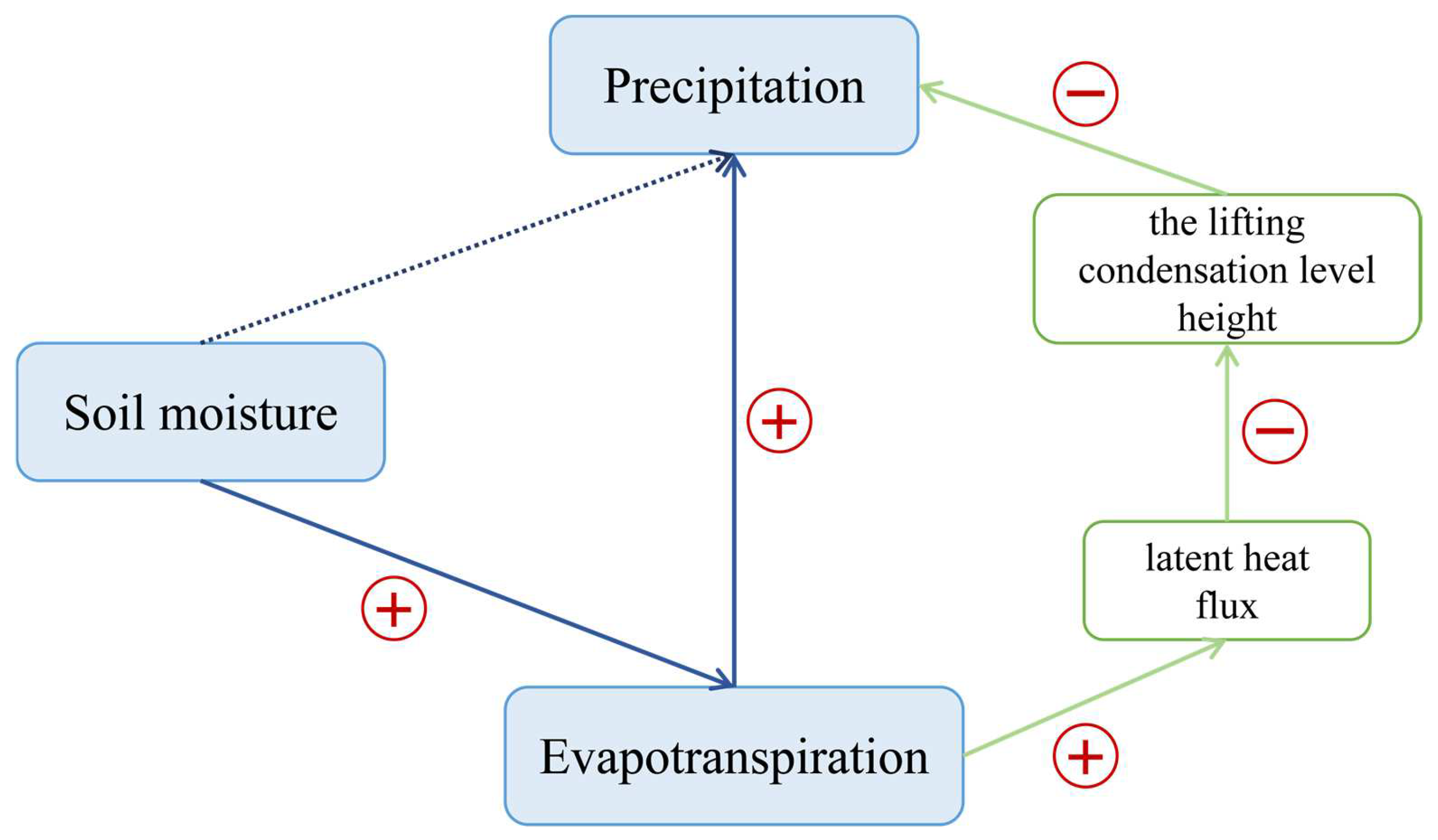
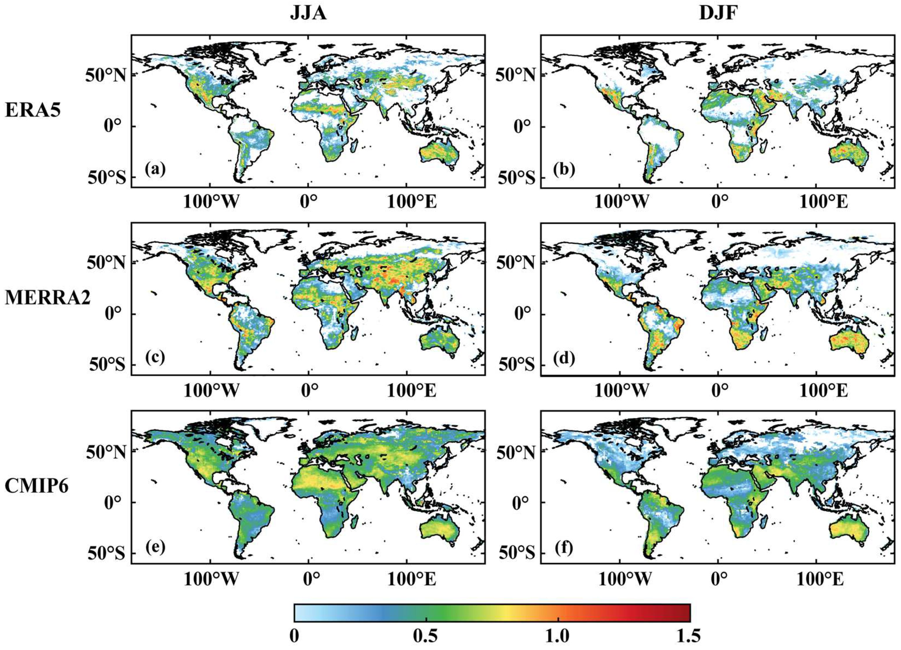
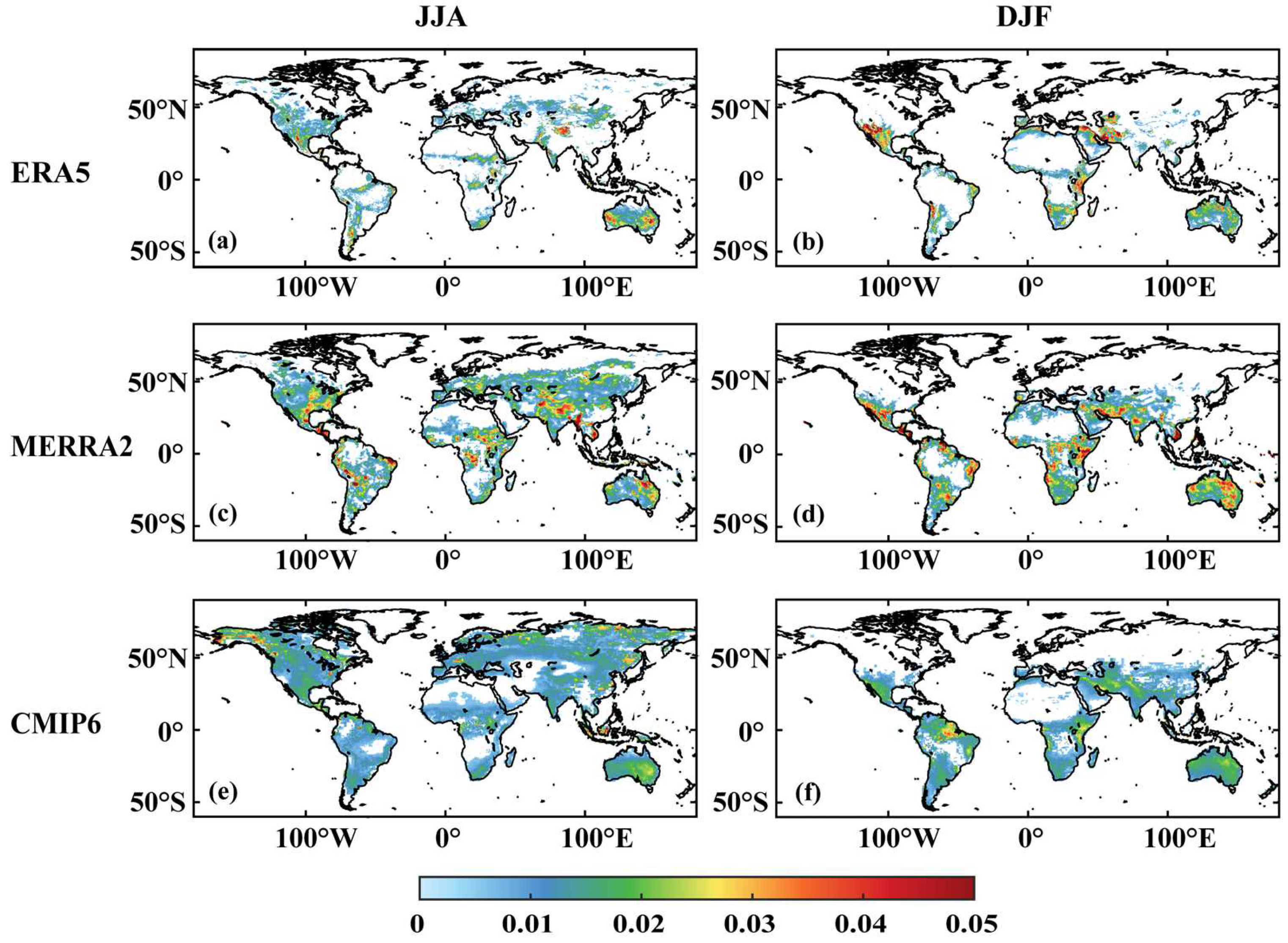
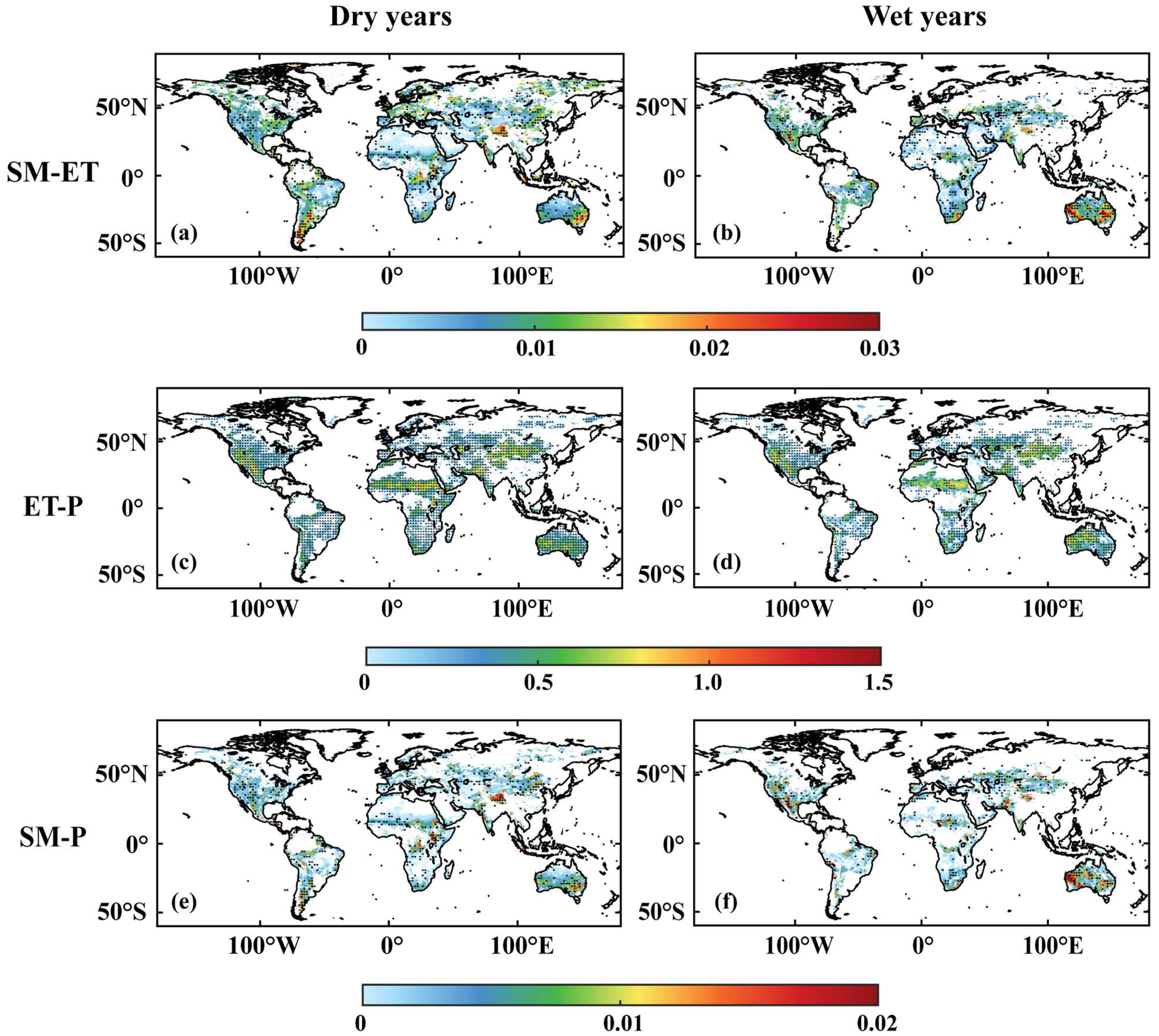
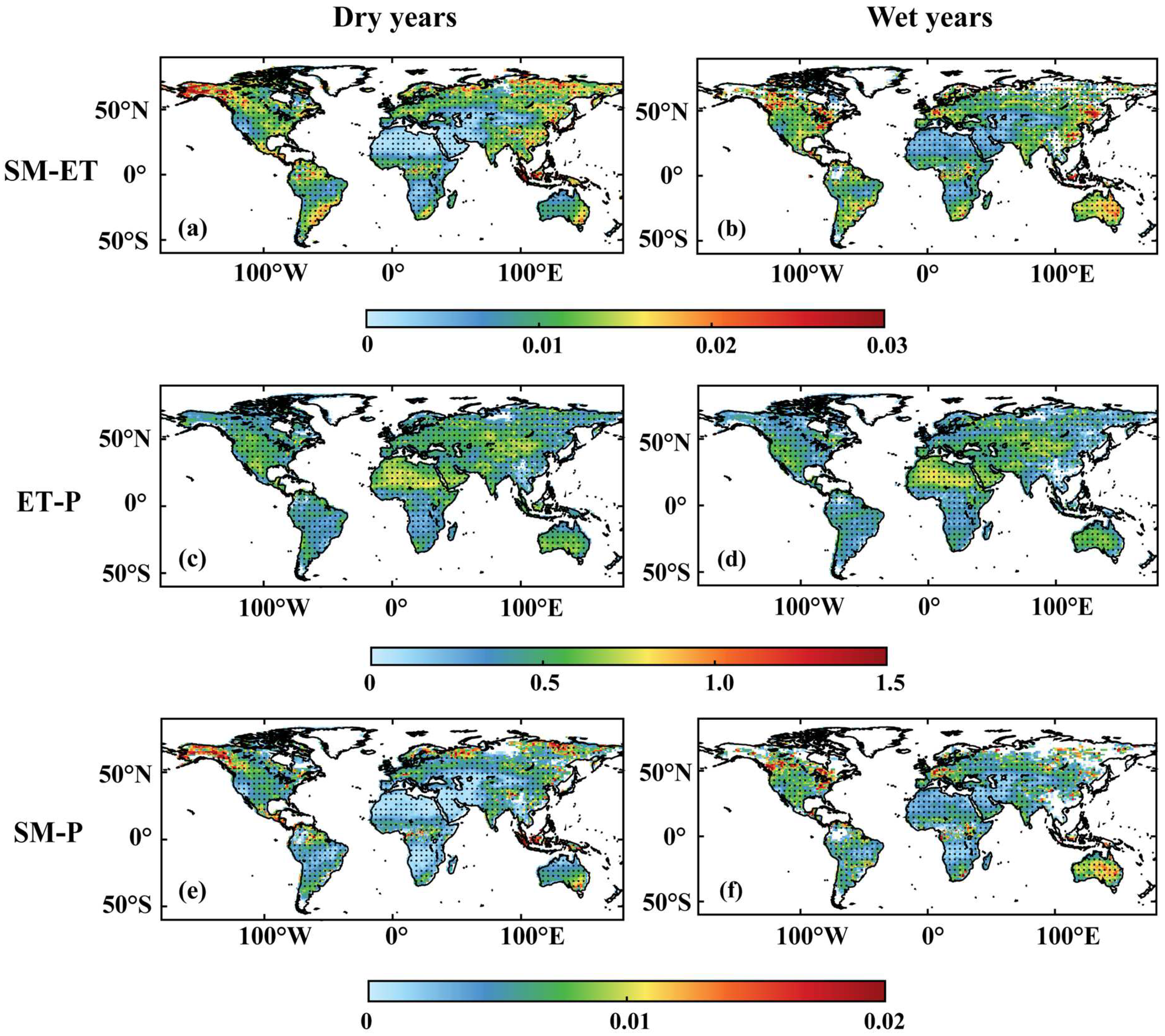
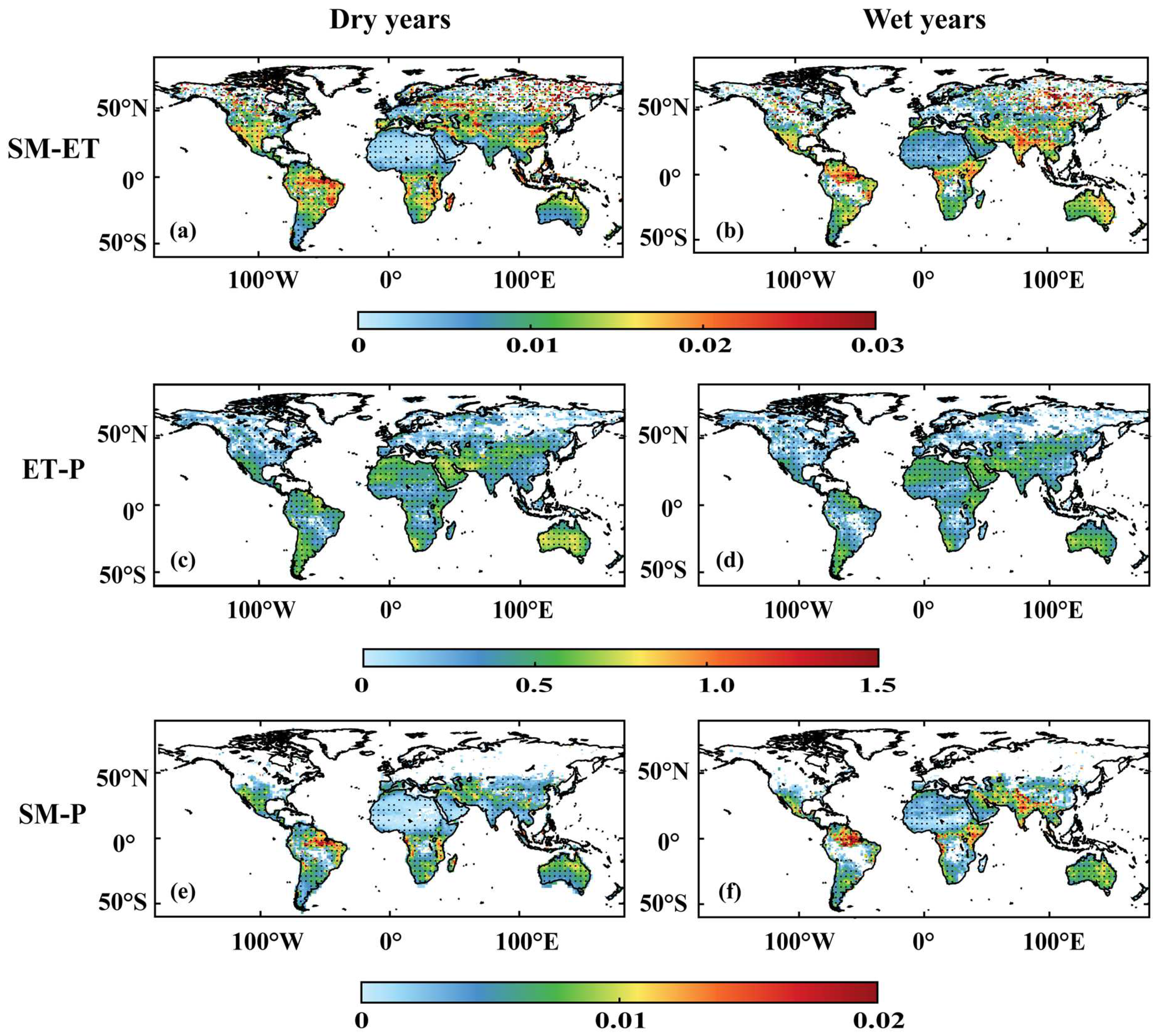
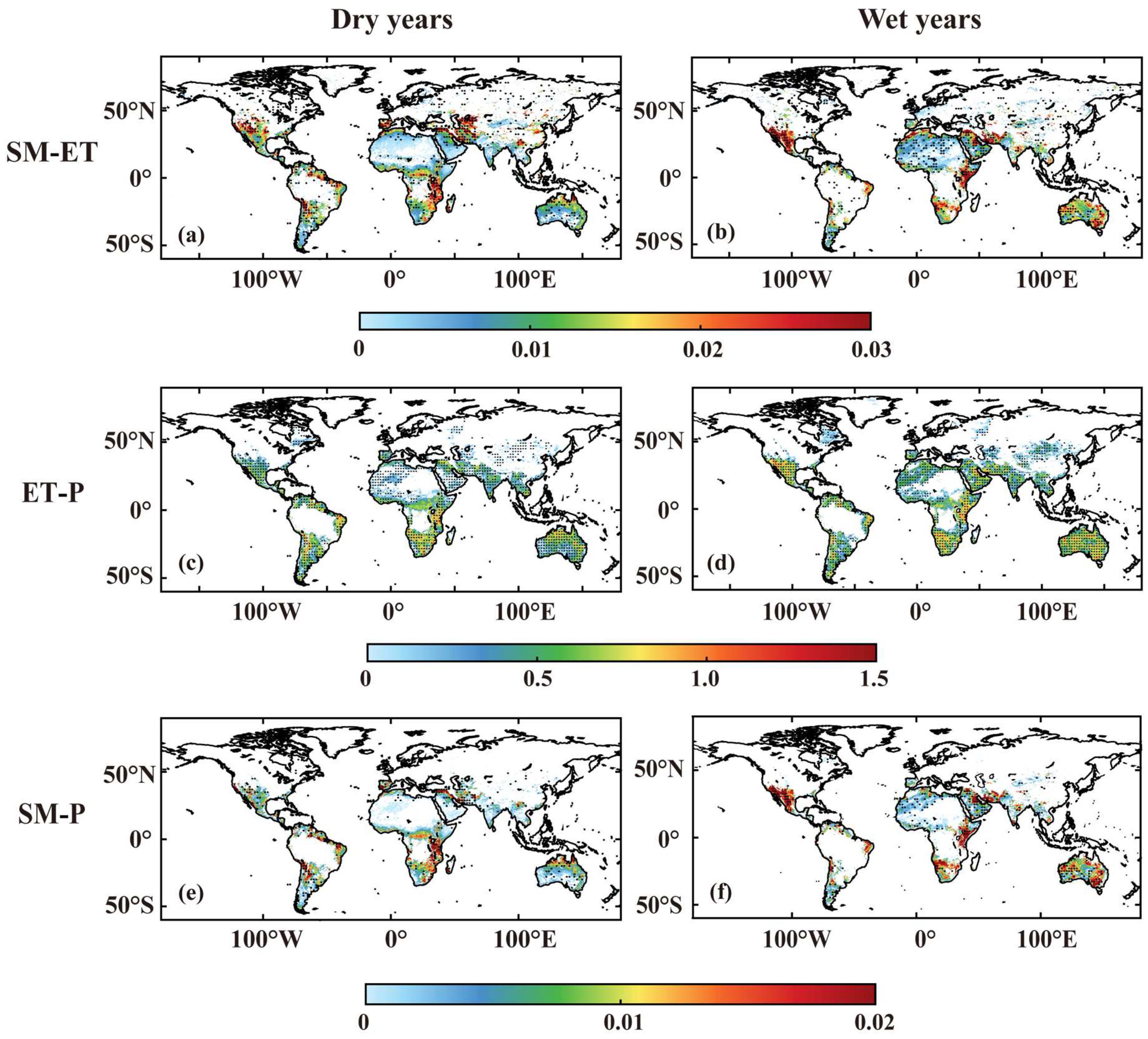
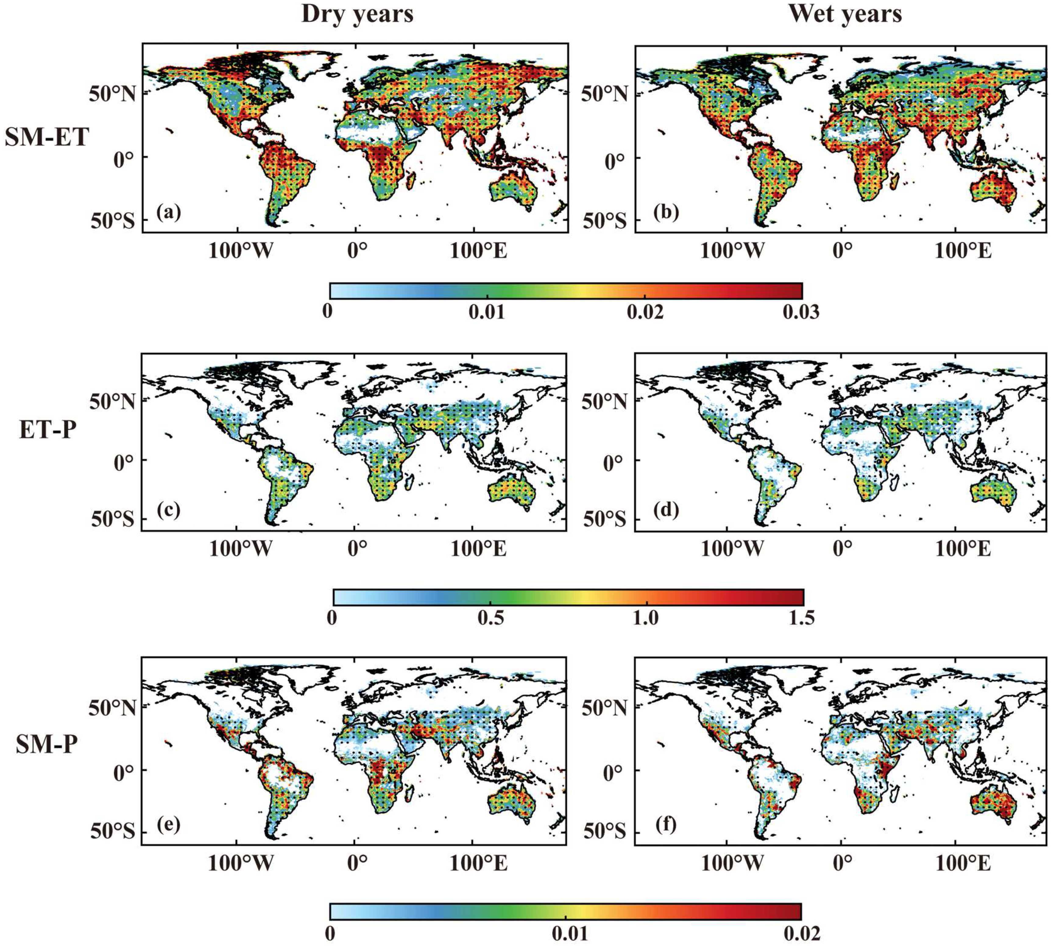
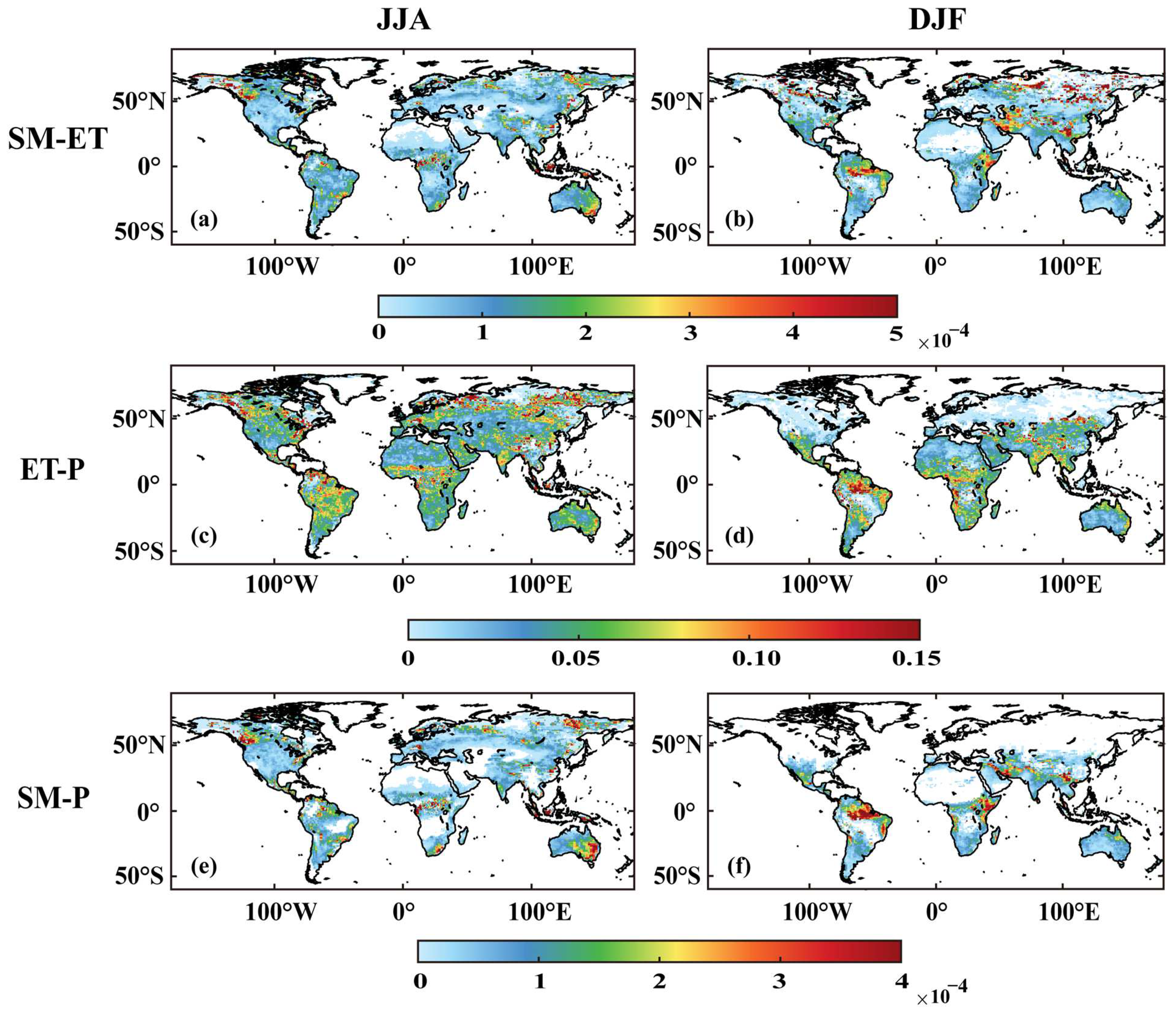
3.1. Dissecting the SM-P Coupling

In Figure 2, the outcomes of local SM-ET are presented for two distinct seasons (JJA and DJF). The shaded regions, referred to as the hotspot regions, indicate a positive correlation between SM and ET. Evidently, ET is influenced by SM, establishing SM as the controlling factor and ET as the responsive factor. As anticipated, JJA exhibits a broader array of hotspot regions in the northern hemisphere as compared to DJF. However, this disparity does not necessarily imply a greater sensitivity. For instance, in North America, JJA demonstrates a more extensive range of hotspot regions compared to DJF, highlighting a heightened ET sensitivity to SM. Furthermore, the equatorial regions display a stronger sensitivity during DJF than during JJA. The distribution of regions with pronounced values in JJA and DJF also differs. Notably, there seems to be a southward shift of hotspot regions during DJF in comparison to JJA.
In addition, the collective potency of SM-ET in CMIP6 models is weaker than in reanalysis data sets. This observation might indicate diminished sensitivities of ET to SM within the CMIP6. In contrast, ERA5 portrays a narrower and more widely scattered array of hotspot regions compared to the other two data sets. The three data sets predominantly share a similar distribution pattern concerning regions with substantial SM-ET. Our findings indicate that regions displaying pronounced SM-ET primarily exist within the transition regions. This outcome aligns with prior investigations that have emphasized the increased sensitivity of ET to SM in these transition regions [13,14,26]. In wet climates characterized by ample SM, ET is not predominantly constrained by SM levels but by the net radiation balance [6,26,48]. In such scenarios, surface radiation primarily drives ET, rendering it the principal governing factor. Within these regions, the influence of SM on P is not expected. Distinct dissimilarities emerge among the three data sets concerning the regional dispersion of SM-ET. To illustrate, within the southeastern coastal region of China, ERA5 and MERRA2 demonstrate feeble or even absent signals, whereas CMIP6 exhibits robust feedback in this specific region. Additionally, CMIP6 showcases pronounced SM-ET at high latitudes, starkly contrasting the absence of such signals in the reanalysis data sets. Moreover, our analysis also reveals that MERRA2 exhibits the most pronounced SM-ET in mid-latitudinal regions, surpassing both ERA5 and CMIP6 in strength.
Following our investigation into SM-ET, we shifted our focus to the atmospheric component, ET-P, which constitutes the second part of SM-P. It can be argued that a lower (higher) LCL height implies reduced (elevated) cloud cover, leading to augmented (diminished) moisture, and subsequently, increased (decreased) precipitation as well [40]. This concept connects surface fluxes to atmospheric conditions and facilitates a more comprehensive exploration of ET-P. Consequently, we analyze the derivative of P concerning ET (ET_pre), which further underscores the sensitivity of precipitation to ET variations. We amalgamate LH-LCL and ET_pre to quantitatively assess ET-P.
The LH-LCL analysis presented here examines the correlation between LH and LCL height. Under wet climatic conditions, changes in LH predominantly respond to alterations in cloud masses and downward solar radiation linked variations in with LCL height. This situation is depicted in regions where the LH-LCL correlation is positive. In these regions, shifts in LH exert relatively minor influence on LCL, primarily indicating the impact of LCL on LH (associated with the energy-limited ET mechanism). Conversely, in semi-arid climatic conditions, a strong negative correlation exists between LH and LCL due to interrelated water and energy fluxes. This establishes a feedback loop that leads to an inverse LH-LCL. In this context, a negative correlation between LH and LCL signifies that LH has the potential to influence LCL height, particularly under water-limited ET conditions [40]. Given this understanding, our ET-P calculations predominantly consider scenarios with negative LH-LCL correlations.
Notably, in Figure 3a, positive correlations dominate in high latitudes, particularly in northern Russia. Negative correlations prevail in semi-arid regions and the transition regions. Comparatively, MERRA2 displays the largest negative correlation region and a smaller positive correlation region concentrated at high latitudes. For instance, concerning Southeast China, ERA5 and CMIP6 exhibit mainly positive LH-LCL correlations, whereas MERRA2 predominantly showcases negative correlations. This outcome aligns with the results from Wei et al. [40], who also utilized MERRA2. Additionally, the region of positive LH-LCL correlation expands and shifts southward from JJA to DJF.
Based on the LH-LCL findings, its spatial arrangement appears to be connected with the spatial distribution of mean P and humidity. The LH-LCL correlation tends to transition from negative to positive as P increases. This observation suggests that negative correlations prevail in dry and transition regions, whereas positive correlations dominate in wetter locales. The results from CMIP6 models align closely with this pattern, mirroring those of ERA5. In contrast, MERRA2 displays notably lower positive LH-LCL correlations compared to ERA5 and CMIP6, with an overall prevalence of negative correlations. This alignment with the results in Figure 3a implies heightened sensitivity in MERRA2, potentially leading to more widely dispersed significant SM-P. Notably, some CMIP6 models exhibit similar patterns to MERRA2, particularly in JJA of Figure 3b, which could impact the ensemble mean while introducing more diverse SM-P signals globally.
In the context of the water cycle, ET contributes to moisture within the atmospheric boundary layer, inducing moist convection and subsequently enhancing the likelihood of P. However, being a primary moisture source does not inherently guarantee a strong influence of ET on P. Due to the intricate interplay of atmospheric components and moisture origins, the anticipated positive impact of ET on P may not always materialize, and in some cases, even leads to a negative correlation. Focusing on the positive ET_pre component in Figure 4, we observe its spatial distribution generally aligns with the negative LH-LCL component. This consistency is a result of the interconnectedness between ET and LH, as well as the relationship between the LCL height and P. ET and LH are interconvertible, and shifts in LCL height contribute to changes in P. The figure reveals that the negative ET_pre component is predominantly concentrated in high latitudes of northern Asia, Europe, and northern North America. In contrast, most other regions display positive ET_pre component, particularly pronounced in MERRA2 and CMIP6 data sets. This pattern suggests potentially more diverse ET-P and SM-P, which could affect the distribution of significant regions. As a product of the two components, ET_pre and LH-LCL are used as necessary but insufficient conditions for ET-P. Here, ET is assumed to be the controlling factor, and P is the responding factor. In Figure 5, hotspot regions are mainly found in dry regions and transition regions. ET-P continues to have significant seasonal variability.
The SM-P feedback mechanisms differ under different conditions. Primarily, SM plays a vital role in generating precipitation through ET under specific circumstances. SM serves as a direct water vapor source for atmospheric P, thereby becoming integral to the water cycle dynamics [2,49]. Wet soils produce high ET and provide water vapor for P [46]. However, the effect of low ET rates on P could be limited [6]. In addition, another indirect interaction of SM and P has been noted in regions where the SM changes the atmospheric boundary layer conditions for cloud-forming rainfall [50,51,52,53,54]. This feedback mechanism underscores the indirect influence of soil moisture, distinct from the inherent dynamics of the water cycle [55,56].
SM-P is derived from the interaction of SM-ET and ET-P components (Figure 6). The significant regions in the figure show where the sensitivity of P to SM is significant. The SM-ET and ET-P exhibit coherent fluctuations when both SM is adequate for ET and the atmosphere contains sufficient water vapor to support precipitation, altering the atmospheric state to foster cloud formation and subsequent rainfall under certain conditions [4,57]. Significantly, the significance of SM-P emerges only when both SM-ET and ET-P exhibit significance. This observation suggests that in scenarios where ET-P lacks significance, the propagation of signals from SM to ET is not sufficient. For instance, during JJA in the Middle East, SM-ET exhibits significance (though weaker in ERA5), yet the combined effect breaks down due to the second component, ET-P. The notable SM-P hotspots are primarily situated in intermediate transition regions and display conspicuous seasonal variability. During JJA, elevated SM-P values are concentrated in southern North America, the Central Asian belt (weaker in ERA5), Eastern Australia, and across the Sahelian belt.
In DJF, the hotspot regions shift southwards, as expected, compared to JJA and intensify in some regions (southern South America, the Middle East, Northern Australia, and Southern Africa). The seasonal variability of SM-P is also indicated by the increase in some regions (southern South America, Middle East, Northern Australia, Southern Africa). Collectively, the SM-P appears weaker in CMIP6 than in the reanalysis data sets, despite being more dispersed, extending to certain wet regions within high-latitude regions of the Northern Hemisphere. Similar to JJA, MERRA2 demonstrates the strongest SM-P among the three data sets in most regions. This mainly reflects the large variation in P sensitivity to SM among the data. As noted earlier, we expect more spread in MERRA2 and CMIP6 due to the strong correlations between LH and LCL, which is seen in the SM-P distributions in Figure 6.

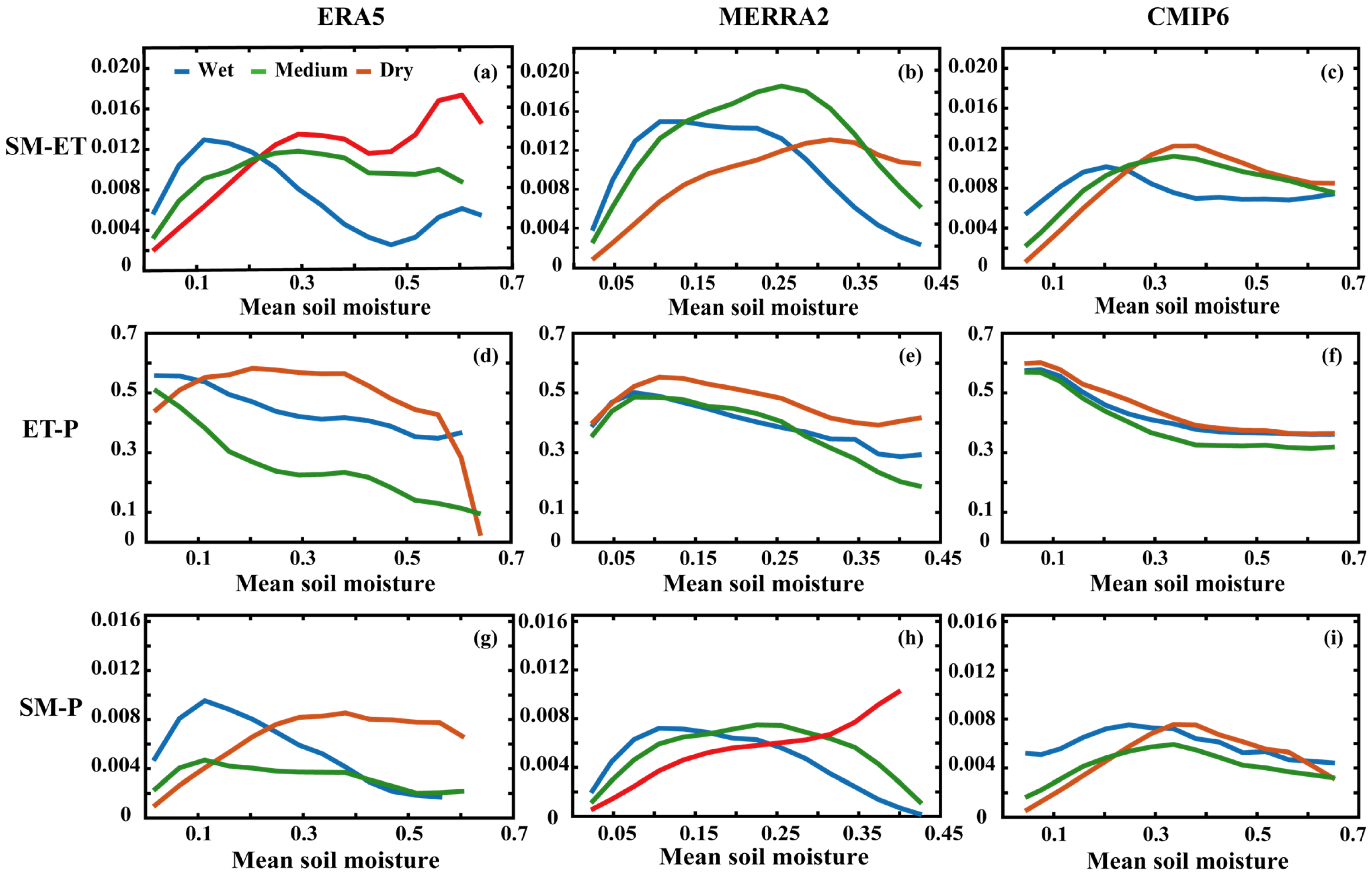
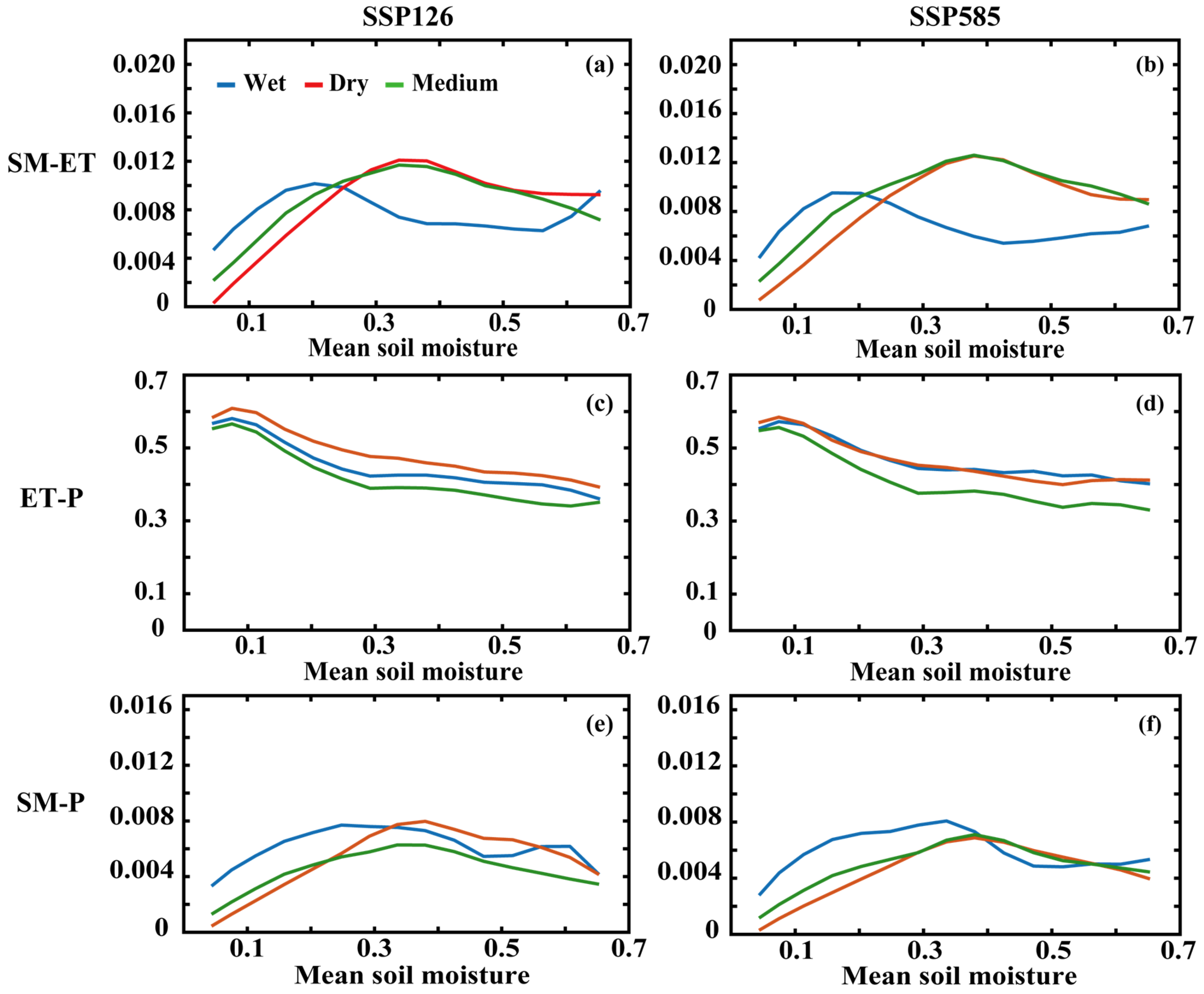
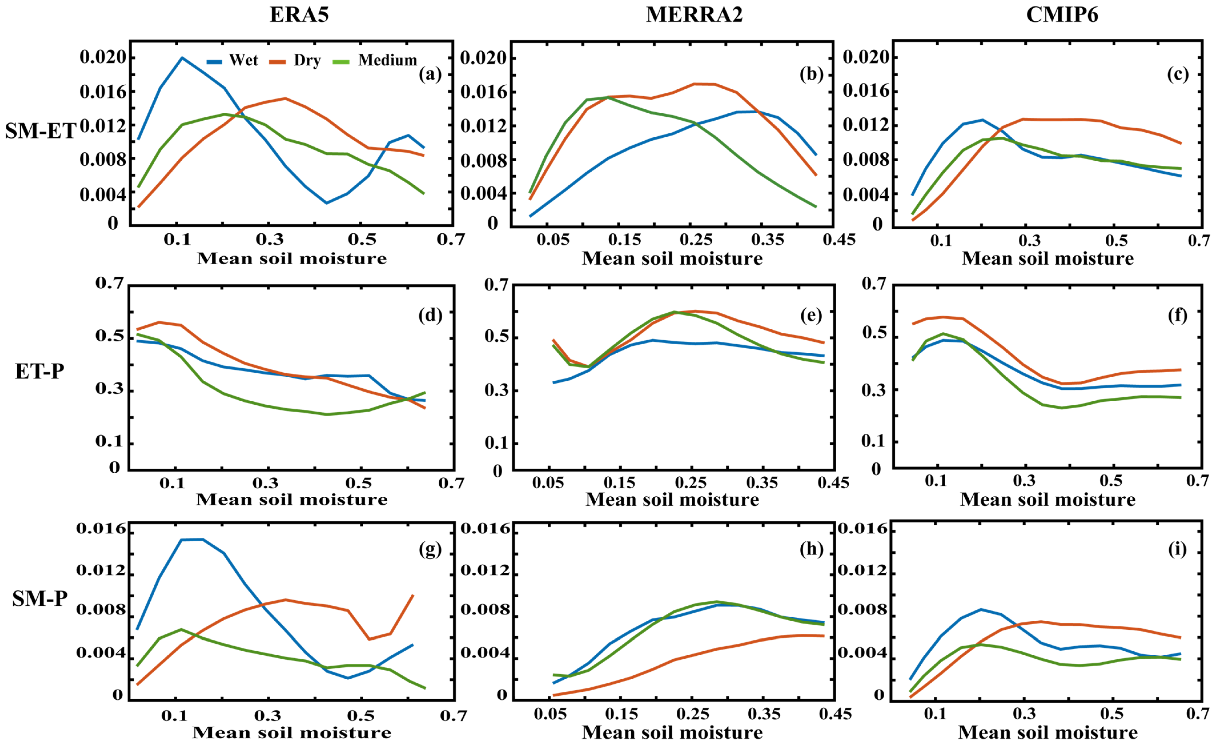
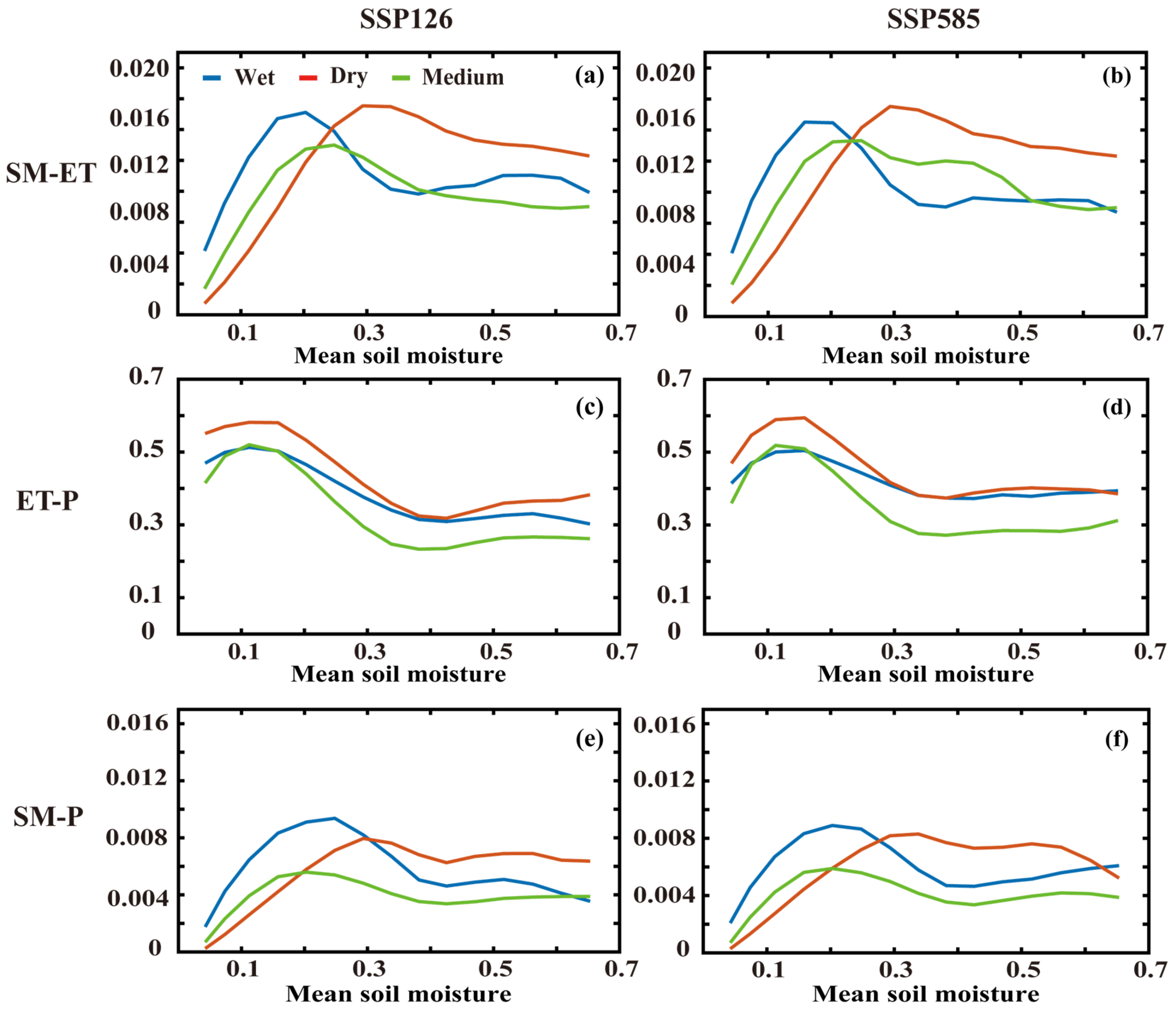
3.2. Variation of SM-P with SM

Studies have shown that the strengths and distribution of SM-P influence and are influenced during anomalously wet and dry conditions. The results for ERA5 are mainly shown in Figure 7, while DJF for ERA5 and both seasons for the CMIP6 and MERRA2 data sets are shown in the Appendix A (Figure A1, Figure A2, Figure A3, Figure A4 and Figure A5). All grid points are divided into dry and wet years according to SM. The findings reveal that SM-ET has a greater sensitivity of ET to SM in wet regions in dry years (Northern South America, Southeast Asia, Southeast Australia) and a greater sensitivity of ET to SM in dry regions in wet years (Central Australia, North Africa, the Middle East). Furthermore, the most prominent signals are concentrated in transition regions where SM plays a substantial role in influencing P patterns. This underscores the significance of comprehending regions with robust SM-P connections. Moreover, the outcomes suggest that under these anomalous SM conditions, SM-P is primarily driven by SM-ET rather than ET-P. The results for JJA and DJF in the two reanalysis data sets are also presented in Figure A1, Figure A2, Figure A3, Figure A4 and Figure A5. These additional figures reveal that precipitation sensitivity to soil moisture in CMIP6 extends to more locations during both dry and wet years compared to the reanalysis data sets.
Figure 8 shows the results for JJA and DJF in Figure A6. SM-ET and SM-P exhibit a characteristic rising and falling structure, both peaking at intermediate SM levels. For wet years, the values of SM-ET and SM-P are elevated in dry regions which contrasts dry years having higher values in wet regions. The strength of the dry-mid-wet couplings of ET-P is influenced by LH-LCL, with high values occurring in regions of lower SM and lower values of ET-P the higher the SM. ET-P showed a gradual decrease from dry to wet regions, with MERRA2 showing a tendency to rise first at low SM. This was particularly evident at DJF, where high values of ET-P occurred in the transition regions. The reason for this is probably because the LH-LCL of MERRA2 is dominated by negative values in both dry and wet regions (Figure 3). As a result, ET-P is less limited by the LH-LCL and this variation is mainly attributed to ET_pre (Figure 4). Furthermore, ET-P consistently exhibits higher values during wet years compared to dry years. This discrepancy is potentially attributed to the greater influence of ground fluxes on the atmospheric state (mainly lifting condensation level, LCL) under drier conditions. Regardless of JJA and DJF, the SM-P structure in the three data sets is closer to SM-ET.

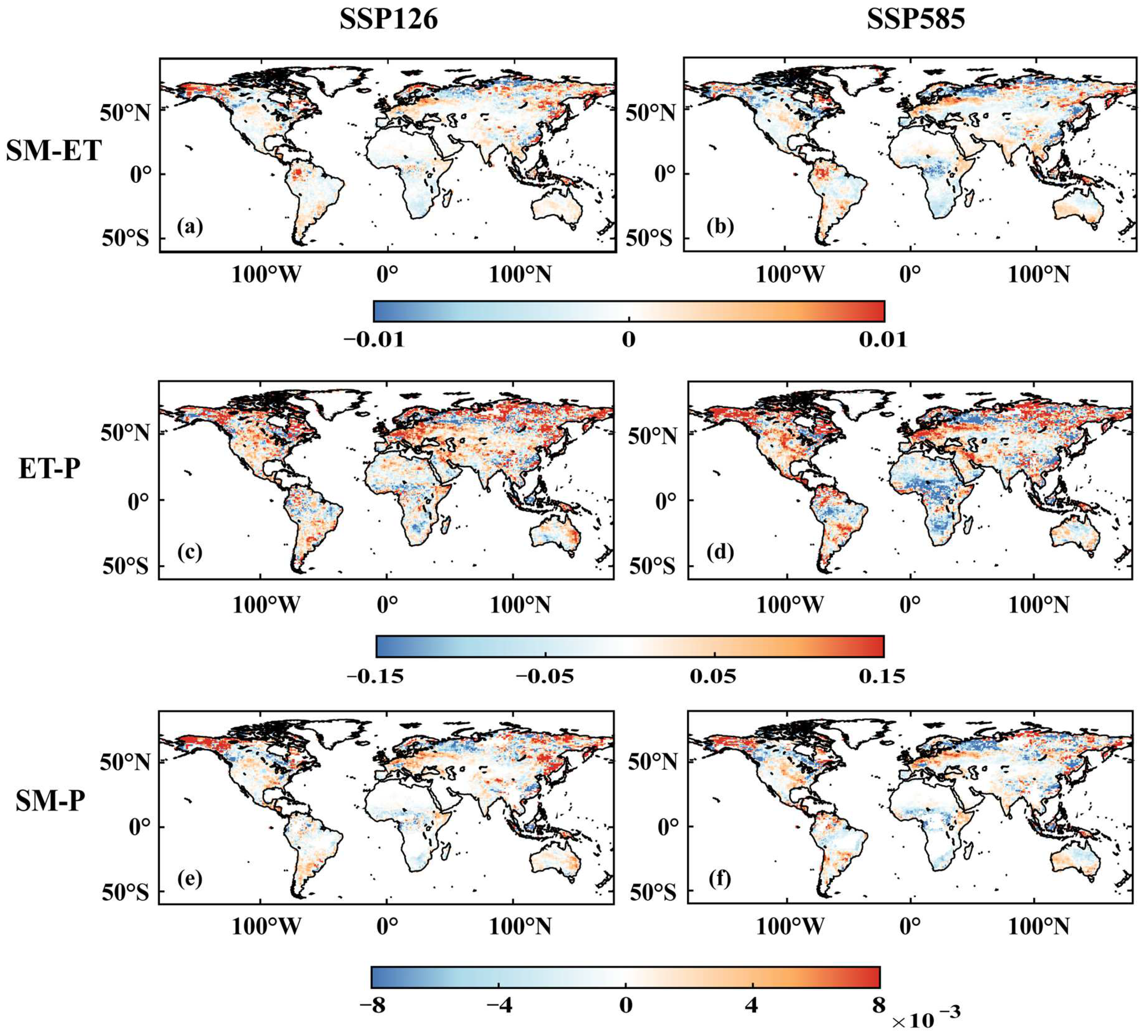
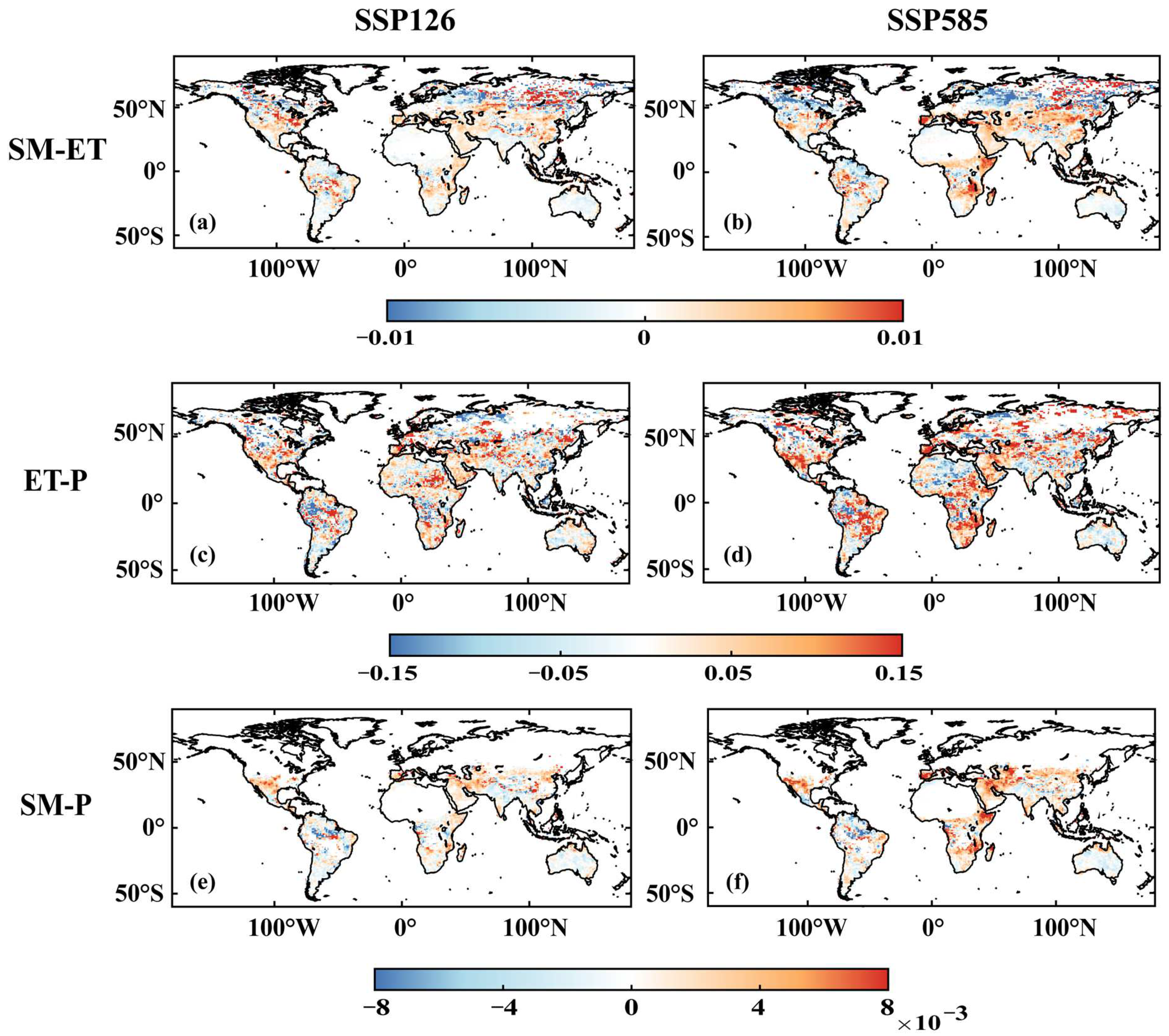
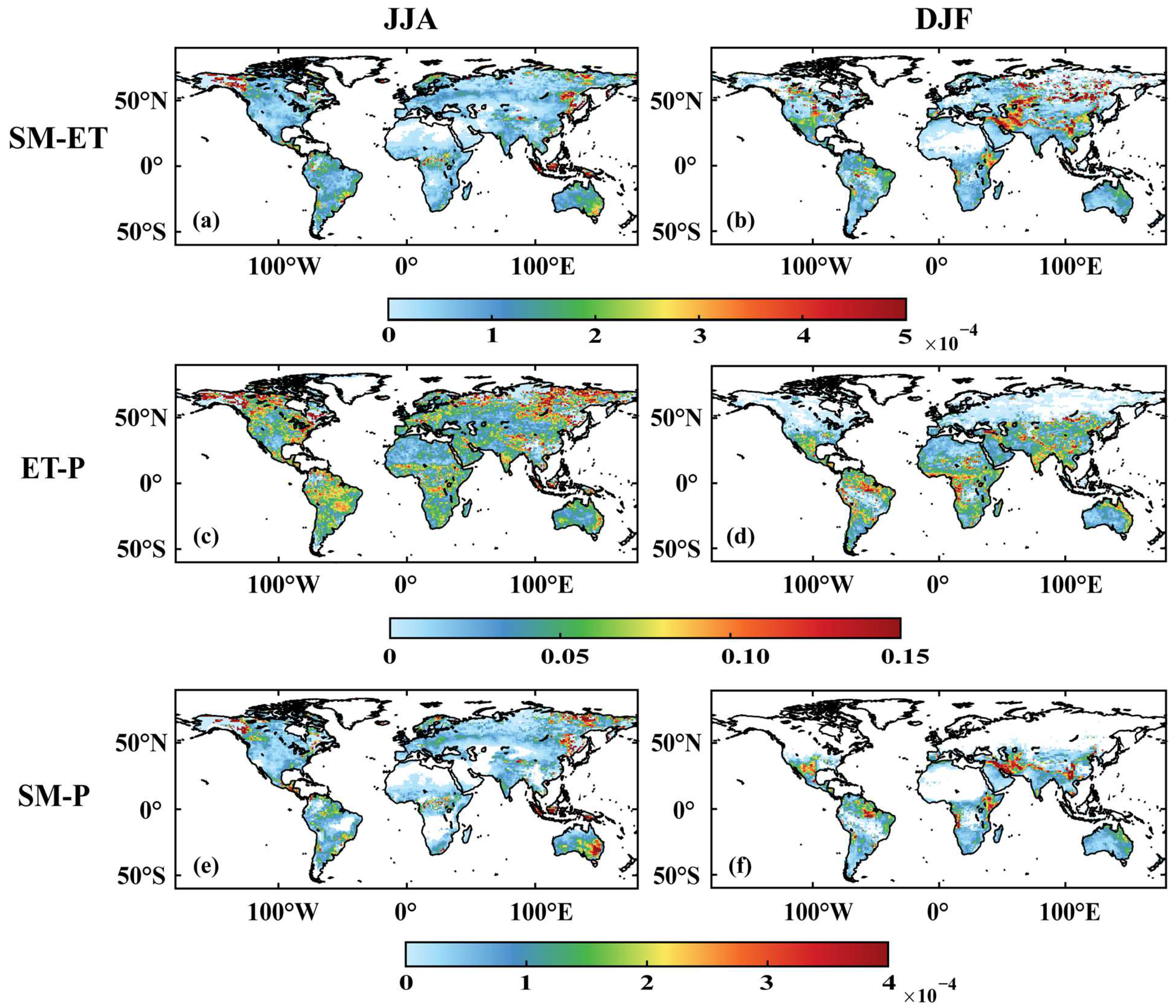
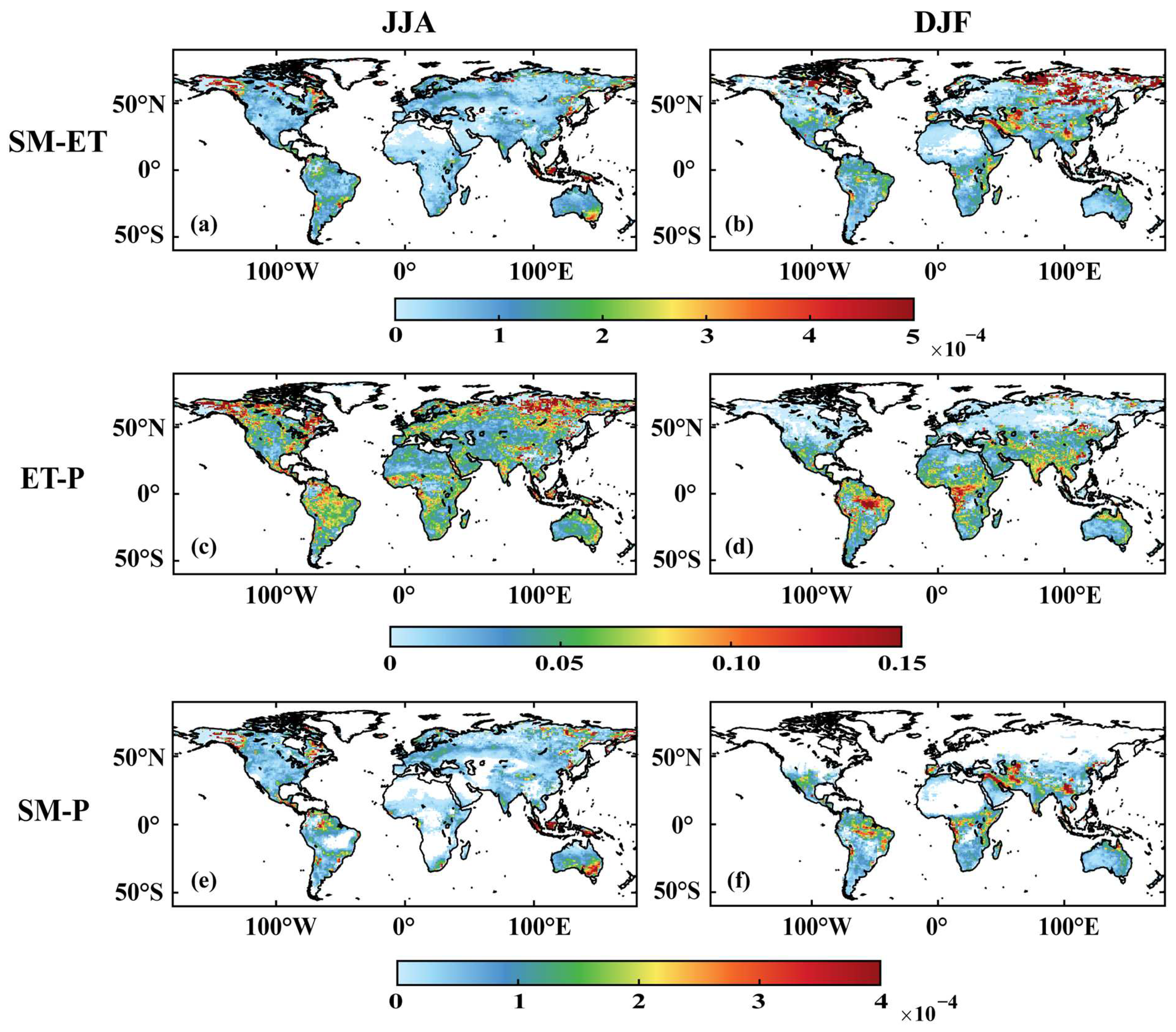
3.3. The SM-P’s Future Changes

So far, the study has focused on the historical period; however, it is also crucial to identify the impact of global warming on the SM-P. The CMIP6 archives make it possible to identify the impact of different pathways of warming on the coupling and its components. Figure 9 depicts the three coupling metrics using data for the last 35 years of the century (2066–2100), compared to the historical 35 years (1980–2014), and uses a sliding window to observe trends. Figure 9a shows the global average of the three coupled metrics (excluding Antarctica and Greenland) calculated using Equation (1). We chose two scenarios, SSP126 and SSP585, as future scenarios to study future changes under different carbon emissions. In DJF, there is a clear upward trend from the historical analysis to the future scenarios, indicating that the sensitivity of precipitation (P) to soil moisture (SM) increases with increasing emissions. Moreover, the SM-P increases in DJF seem to be more strongly determined by changes in ET-P than changes in SM-ET, which are smaller. Berg et al. [58,59] recently found that changes in atmospheric components of land–atmosphere feedback are more strongly impacted than the land component. These earlier findings offer insight into why we observe comparatively smaller changes in SM-ET as opposed to ET-P.
On the other hand, during JJA, although there is an increase in the future, these changes are relatively similar for both SSP126 and SSP585. In addition, the changes observed during JJA are minimal compared to DJF. This regional perspective aids in uncovering the varying patterns of sensitivity across different regions under different emission scenarios and seasons. Our investigation revealed distinct patterns of enhancement and attenuation for the three coupling metrics across various regions. Notably, the SSP585 scenario demonstrated a tendency toward strengthening these metrics. Regions where SSP126 showed weakening tendencies also experienced even greater weakening under SSP585, and similarly, regions that strengthened under SSP126 exhibited further amplification in their coupling metrics under SSP585. These dynamics collectively contribute to a more subdued alteration in the three coupling metrics when evaluated through global average analysis. These observations could potentially be linked to recent findings concerning anticipated changes in atmospheric circulation patterns under different warming pathways, as reported by Chemke et al. [60] and Lachmy [61]. These shifts in atmospheric circulation consequently impact ET-P, resulting in changes within the SM-P. In Figure 9b, the three coupling metrics are computed using a sliding window of 11 years. The graph illustrates that SM-ET and SM-P do not exhibit significant changes over time, whereas ET-P displays a more distinct upward trend. The pattern of change observed in SM-P closely mirrors that of SM-ET. However, it is essential to recognize that the strength of these changes may differ when employing various sliding window lengths.
To facilitate better comparison, historical SM data were retained for use in the future analysis. The similarity between the curves of the two future indicators (SSP126, SSP585) and the historical data is clearly evident in Figure 10. Both SM-ET and SM-P showcase higher values wherein wet climate regions during dry years, and the converse occurs in dry regions. This also indicates a high degree of consistency with history in regions sensitive to future P. The main strength differences exist among the historical SSP126 and SSP585. Against the historical JJA, SM-ET and SM-P are significantly enhanced mainly in the middle years of the transition regions. Additionally, SSP585 shows even greater enhancement compared to SSP126. In Figure A9 (Appendix A), the overall enhancement of SM-ET is more pronounced compared to the historical DJF. Once again, SSP585 demonstrates greater enhancement in comparison to SSP126, reflecting the substantial impact of future high carbon emissions on land–atmosphere interactions. Conversely, the strength of ET-P displays only minor variations in the future during both JJA and DJF. Moreover, the structure of SM-P largely remains under the control of SM-ET, maintaining consistency with historical patterns.

4. Discussion

The current study analyzes global hotspots of SM-P as a function of the sensitivity of P to changes in SM. We sought to unravel the distinct contributions of the terrestrial and atmospheric components within the SM-P framework. Additionally, we explored how these three coupling metrics vary with different climate conditions. The uniqueness of this study is that it relies on the LCL height as an integral part of the SM-P continuum. The LCL height serves as a close proxy for mean cloud base height and can be used as a good approximation or indicator of precipitation probability [32]. Thus, by including it, we fill in the gaps of earlier SM-P coupling studies and aim to understand how this is represented in multiple climate models. We include three different families of data sets from different sources in the analysis, two sets of which are reanalysis data sets and the third, multiple climate models of the CMIP framework. By comparing the SM-P coupling based on Equation (1), we aim to understand the different representations of the coupling in these data sets. It is imperative to recognize that SM-P interactions are influenced by many complex factors, and their mutual interactions are intricate. This complexity has posed formidable challenges in establishing robust cause-and-effect relationships. Our research, at its current stage, has delved into the positive feedback loops associated with SM-P coupling, but the exploration of negative feedback loops warrants deeper investigation. It is our intention that future studies in this field will extend their focus beyond the local effects and delve into the intricacies of non-local effects. This expansion of research scope will enable a more comprehensive understanding of the multifaceted dynamics governing SM-P interactions, ultimately contributing to advancing our knowledge in this critical area of study.
In the context of global warming, future changes in land–atmosphere interactions are also an issue of concern. Therefore, we use CMIP6 models output variables to investigate future SM-P. The reasons regarding future changes are perhaps complex. Certain studies have proposed that the expansion of the Hadley circulation is anticipated in the 21st century, predominantly under anthropogenic influence [62,63,64]. In contrast, at mid-latitudes, non-adiabatic heating (the process of heat exchange between the system and the outside world) is evident within the ascending branch of the Ferrel Cell [65]. This phenomenon leads to a clockwise, lower tropospheric circulation of the Ferrel Cell that intensifies and shifts poleward in light to climate change [61]. From our findings, it is evident that there is a significant amplification of SM-P interactions, particularly within the atmospheric segment, in mid-latitude regions. This means that with climate change, we must take into account the influence of circulation factors on the atmospheric state and land surface atmospheric interactions when analyzing future long-term changes and thus the mechanisms of change. Incorporating these insights into climate models and adaptation strategies will be essential for addressing the complex and dynamic challenges of a changing climate in mid-latitude regions and beyond.

5. Conclusions

This study employs a novel SM-P framework to delve into its feedback mechanisms. The results indicated that the hotspot regions of SM-P are predominantly situated within the transition regions, with significant seasonal variations. In wet climate regions, both SM-ET and SM-P showed elevated levels during dry years compared to wet years, while the reverse was also true in dry climate regions. This demonstrates that SM exerts a stronger influence on P over intermediate transition regions, consistent with previous studies [4,6,13,14]. Both SM-ET and SM-P demonstrated their peak values within these transition regions, thereby revealing a spatial pattern similarity between the two. Upon partitioning the years into wet and dry categories, it became apparent that SM-P and SM-ET exhibited comparable temporal variability. Significantly, the SSP585 scenario exhibited a notable inclination toward enhancing these metrics. Areas where the SSP126 scenario indicated a weakening trend experienced even more pronounced weakening under SSP585. Conversely, regions that displayed strengthened coupling metrics under SSP126 exhibited further amplification of these trends when subjected to SSP585. Due to sensitivity to climate change, the ET-P exhibits a more pronounced upward trend in the future. This approach could offer a simplified yet meaningful means of comprehending the intricate interplay between SM and P within different climate regimes. Future research may benefit from incorporating additional variables and higher-resolution data to provide a more comprehensive understanding of SM-P interactions in diverse environmental settings.

Author Contributions

Conceptualization, X.Z., G.W., D.F.T.H. and S.L.; Funding acquisition, G.W.; Methodology, X.Z., D.F.T.H. and J.W.; Supervision, G.W.; Validation, X.Z., G.W. and D.F.T.H.; Writing—original draft, X.Z.; Writing—review & editing, X.Z., D.F.T.H., S.L., J.W., J.L., Y.Q., C.Z., W.U. and E.Y. All authors have read and agreed to the published version of the manuscript.

Funding

This research was funded by the National Nature Science Foundation of China, grant number 42275028 and the Sino-German Cooperation Group Program, grant number GZ1447.

Institutional Review Board Statement

Not applicable.

Informed Consent Statement

Not applicable.

Data Availability Statement

Data from the fifth generation ECMWF reanalysis for the global climate and weather for the past 8 decades (ERA5) can be accessed through https://www.ecmwf.int/en/forecasts/datasets/reanalysis-datasets/era5, accessed on 14 February 2022. Data from the Modern Retrospective Analysis for Research and Applications, Version 2 (MERRA2) can be accessed through https://gmao.gsfc.nasa.gov/reanalysis/MERRA-2/, accessed on 22 March 2022. Data from the World Climate Research Programme (WCRP) Coupled Model Intercomparison Project Phase 6 (CMIP6) can be accessed through https://esgf-node.llnl.gov/projects/cmip6/, accessed on 6 January 2022.

Conflicts of Interest

The authors declare no conflict of interest.

Appendix A

Figure A1. The SM-ET, ET-P, and SM-P against mean soil moisture change during JJA for CMIP6 in dry and wet years. The soil moisture is standardized (SMn) and the calculation criteria for the colored part of the figure are: SMn > 0 are taken as wet years and SMn < 0 are taken as dry years. On the basis of these divisions the regions where the calculation criteria are >1 for wet years and <−1 for dry years are highlighted, as indicated by points. (a,b) indicate the SM-ET in wet and dry years, respectively. (c,d) indicate the ET-P. (e,f) indicate the SM-P.
Atmosphere 14 01531 g0a1
Figure A2. The SM-ET, ET-P, and SM-P against mean soil moisture change during DJF for CMIP6 in dry and wet years. The soil moisture is standardized (SMn) and the calculation criteria for the colored part of the figure are: SMn > 0 are taken as wet years and SMn < 0 are taken as dry years. On the basis of these divisions the regions where the calculation criteria are >1 for wet years and <−1 for dry years are highlighted, as indicated by points. (a,b) indicate the SM-ET. (c,d) indicate the ET-P. (e,f) indicate the SM-P.
Atmosphere 14 01531 g0a2
Figure A3. The SM-ET, ET-P, and SM-P against mean soil moisture change during DJF for ERA5 in dry and wet years. The soil moisture is standardized (SMn) and the calculation criteria for the colored part of the figure are: SMn > 0 are taken as wet years and SMn < 0 are taken as dry years. On the basis of these divisions the regions where the calculation criteria are >1 for wet years and <−1 for dry years are highlighted, as indicated by points. (a,b) indicate the SM-ET. (c,d) indicate the ET-P. (e,f) indicate the SM-P.
Atmosphere 14 01531 g0a3
Figure A4. The SM-ET, ET-P, and SM-P against mean soil moisture change during JJA for MERRA2 in dry and wet years. The soil moisture is standardized (SMn) and the calculation criteria for the colored part of the figure are: SMn > 0 are taken as wet years and SMn < 0 are taken as dry years. On the basis of these divisions the regions where the calculation criteria are >1 for wet years and <−1 for dry years are highlighted, as indicated by points. (a,b) indicate the SM-ET. (c,d) indicate the ET-P. (e,f) indicate the SM-P.
Atmosphere 14 01531 g0a4
Figure A5. The SM-ET, ET-P, and SM-P against mean soil moisture change during DJF for MERRA2 in dry and wet years. The soil moisture is standardized (SMn) and the calculation criteria for the colored part of the figure are: SMn > 0 are taken as wet years and SMn < 0 are taken as dry years. On the basis of these divisions the regions where the calculation criteria are >1 for wet years and <−1 for dry years are highlighted, as indicated by points. (a,b) indicate the SM-ET. (c,d) indicate the ET-P. (e,f) indicate the SM-P.
Atmosphere 14 01531 g0a5
Figure A6. The SM-ET, ET-P, and SM-P against mean soil moisture change in wet, medium, and dry years during DJF for ERA5, MERRA2, and CMIP6. Criteria for dry, medium and wet years: The SM is standardized (SMn); grids with −1 <= SMn >= 1 are taken as medium years, grids with SMn < −1 are taken as dry years and SMn > 0 are taken as wet years. (ac) indicate the SM-ET for ERA5, MERRA2, and CMIP6. (df) indicate the ET-P for ERA5, MERRA2, and CMIP6. (gi) indicate the SM-P for ERA5, MERRA2, and CMIP6.
Atmosphere 14 01531 g0a6
Figure A7. The future (2066–2100) from SSP126 and SSP585 versus historical (1980–2014) differences in SM-ET, ET-P and SM-P during JJA. The blue color signifies a weakening of sensitivity, whereas the red color indicates an increase in sensitivity. (a,b) indicate the SM-ET for SSP126 and SSP585, respectfully. (c,d) indicate the ET-P for SSP126 and SSP585, respectfully. (e,f) indicate the SM-P for SSP126 and SSP585, respectfully.
Atmosphere 14 01531 g0a7
Figure A8. The future (2066–2100) from SSP126 and SSP585 versus historical (1980–2014) differences in SM-ET, ET-P, and SM-P during DJF. The blue color signifies a weakening of sensitivity, whereas the red color indicates an increase in sensitivity. (a,b) indicate the SM-ET for SSP126 and SSP585, respectfully. (c,d) indicate the ET-P for SSP126 and SSP585, respectfully. (e,f) indicate the SM-P for SSP126 and SSP585, respectfully.
Atmosphere 14 01531 g0a8
Figure A9. The SM-ET, ET-P, and SM-P against mean soil moisture change in wet, medium, and dry during DJF for SSP126 and SSP585 of CMIP6. Criteria for dry, medium and wet years: The SM is standardized (SMn); grids with −1 <= SMn >= 1 are taken as medium years, grids with SMn < −1 are taken as dry years and SMn > 0 are taken as wet years. (a,b) indicate the SM-ET for SSP126 and SSP585, respectfully. (c,d) indicate the ET-P for SSP126 and SSP585, respectfully. (e,f) indicate the SM-P for SSP126 and SSP585, respectfully.
Atmosphere 14 01531 g0a9
Figure A10. Historical variance of the CMIP6 model for the SM-ET, ET-P, and SM-P, reflecting the uncertainty between the models. The (a,c,e) mean the model variance during JJA for historical. The (b,d,f) mean the model variance during DJF for historical.
Atmosphere 14 01531 g0a10
Figure A11. SSP126 variance of the CMIP6 model for the SM-ET, ET-P, and SM-P, reflecting the uncertainty between the models. The (a,c,e) mean the model variance during JJA for SSP126. The (b,d,f) mean the model variance during DJF for SSP126.
Atmosphere 14 01531 g0a11
Figure A12. SSP585 variance of the CMIP6 model for the SM-ET, ET-P, and SM-P, reflecting the uncertainty between the models. The (a,c,e) mean the model variance at JJA for SSP585. The (b,d,f) mean the model variance at DJF for SSP585.
Atmosphere 14 01531 g0a12

References

  1. Pitman, A.J. The evolution of, and revolution in, land surface schemes designed for climate models. Int. J. Clim. 2003, 23, 479–510. [Google Scholar] [CrossRef]
  2. Seneviratne, S.I.; Corti, T.; Davin, E.L.; Hirschi, M.; Jaeger, E.B.; Lehner, I.; Orlowsky, B.; Teuling, A.J. Investigating soil moisture—Climate interactions in a changing climate: A review. Earth-Sci. Rev. 2010, 99, 125–161. [Google Scholar] [CrossRef]
  3. Wei, J.; Dickinson, R.E.; Chen, H. A Negative Soil Moisture-Precipitation Relationship and Its Causes. J. Hydrometeorol. 2008, 9, 1364–1376. [Google Scholar] [CrossRef]
  4. Koster, R.D.; Mahanama, S.P.P.; Yamada, T.J.; Balsamo, G.; Berg, A.A.; Boisserie, M.; Dirmeyer, P.A.; Doblas-Reyes, F.J.; Drewitt, G.; Gordon, C.T.; et al. The Second Phase of the Global Land–Atmosphere Coupling Experiment: Soil Moisture Contributions to Subseasonal Forecast Skill. J. Hydrometeorol. 2011, 12, 805–822. [Google Scholar] [CrossRef]
  5. Tuttle, S.; Salvucci, G. Empirical evidence of contrasting soil moisture-precipitation feedbacks across the United States. Science 2016, 352, 825–828. [Google Scholar] [CrossRef]
  6. Koster, R.D.; Dirmeyer, P.A.; Guo, Z.; Bonan, G.; Chan, E.; Cox, P.; Gordon, C.T.; Kanae, S.; Kowalczyk, E.; Lawrence, D.; et al. Regions of Strong Coupling between Soil Moisture and Precipitation. Science 2004, 305, 1138–1140. [Google Scholar] [CrossRef] [PubMed]
  7. Bellucci, A.; Haarsma, R.; Bellouin, N.; Booth, B.; Cagnazzo, C.; van den Hurk, B.; Keenlyside, N.; Koenigk, T.; Massonnet, F.; Materia, S.; et al. Advancements in decadal climate predictability: The role of nonoceanic drivers. Rev. Geophys. 2015, 53, 165–202. [Google Scholar] [CrossRef]
  8. Dong, J.; Dirmeyer, P.A.; Lei, F.; Anderson, M.C.; Holmes, T.R.H.; Hain, C.; Crow, W.T. Soil Evaporation Stress Determines Soil Moisture-Evapotranspiration Coupling Strength in Land Surface Modeling. Geophys. Res. Lett. 2020, 47, e2020GL090391. [Google Scholar] [CrossRef]
  9. Eltahir, E.A.B. A Soil Moisture–Rainfall Feedback Mechanism: 1. Theory and observations. Water Resour. Res. 1998, 34, 765–776. [Google Scholar] [CrossRef]
  10. Hu, H.; Leung, L.R.; Feng, Z. Early warm-season mesoscale convective systems dominate soil moisture-precipitation feedback for summer rainfall in central United States. Proc. Natl. Acad. Sci. USA 2021, 118, e2105260118. [Google Scholar] [CrossRef]
  11. Shukla, J.; Mintz, Y. Influence of Land-Surface Evapotranspiration on the Earth’s Climate. Science 1982, 215, 1498–1501. [Google Scholar] [CrossRef] [PubMed]
  12. Notaro, M. Statistical identification of global hot spots in soil moisture feedbacks among IPCC AR4 models. J. Geophys. Res. Atmos. 2008, 113, D09101. [Google Scholar] [CrossRef]
  13. Wei, J.; Dirmeyer, P.A. Dissecting soil moisture-precipitation coupling. Geophys. Res. Lett. 2012, 39, L19711. [Google Scholar] [CrossRef]
  14. Wang, Y.; Yang, J.; Chen, Y.; De Maeyer, P.; Li, Z.; Duan, W. Detecting the Causal Effect of Soil Moisture on Precipitation Using Convergent Cross Mapping. Sci. Rep. 2018, 8, 12171. [Google Scholar] [CrossRef] [PubMed]
  15. Koster, R.D.; Sud, Y.C.; Guo, Z.; Dirmeyer, P.A.; Bonan, G.; Oleson, K.W.; Chan, E.; Verseghy, D.; Cox, P.; Davies, H.; et al. GLACE: The Global Land–Atmosphere Coupling Experiment. Part I: Overview. J. Hydrometeorol. 2006, 7, 590–610. [Google Scholar] [CrossRef]
  16. Wei, J.; Dirmeyer, P.A.; Guo, Z. Sensitivities of soil wetness simulation to uncertainties in precipitation and radiation. Geophys. Res. Lett. 2008, 35, L15703. [Google Scholar] [CrossRef]
  17. Graf, M.; Arnault, J.; Fersch, B.; Kunstmann, H. Is the soil moisture precipitation feedback enhanced by heterogeneity and dry soils? A comparative study. Hydrol. Process. 2021, 35, e14332. [Google Scholar] [CrossRef]
  18. Asharaf, S.; Dobler, A.; Ahrens, B. Soil Moisture-Precipitation Feedback Processes in the Indian Summer Monsoon Season. J. Hydrometeorol. 2012, 13, 1461–1474. [Google Scholar] [CrossRef]
  19. Zhong, S.; Yang, T.; Qian, Y.; Zhu, J.; Wu, F. Temporal and spatial variations of soil moisture-precipitation feedback in East China during the East Asian summer monsoon period: A sensitivity study. Atmos. Res. 2018, 213, 163–172. [Google Scholar] [CrossRef]
  20. Guo, Z.; Dirmeyer, P.A.; Koster, R.D.; Sud, Y.C.; Bonan, G.; Oleson, K.W.; Chan, E.; Verseghy, D.; Cox, P.; Gordon, C.T.; et al. GLACE: The Global Land–Atmosphere Coupling Experiment. Part II: Analysis. J. Hydrometeorol. 2006, 7, 611–625. [Google Scholar] [CrossRef]
  21. Gentine, P.; Holtslag, A.A.M.; D’Andrea, F.; Ek, M. Surface and Atmospheric Controls on the Onset of Moist Convection over Land. J. Hydrometeorol. 2013, 14, 1443–1462. [Google Scholar] [CrossRef]
  22. Wei, J.; Dirmeyer, P.A. Sensitivity of land precipitation to surface evapotranspiration: A nonlocal perspective based on water vapor transport. Geophys. Res. Lett. 2019, 46, 12588–12597. [Google Scholar] [CrossRef]
  23. Yang, Z.; Zhang, Q.; Zhang, Y.; Yue, P.; Zhang, L.; Zeng, J.; Qi, Y. Hydrothermal Factors Influence on Spatial-Temporal Variation of Evapotranspiration-Precipitation Coupling over Climate Transition Zone of North China. Remote Sens. 2022, 14, 1448. [Google Scholar] [CrossRef]
  24. Liu, D.; Yu, Z.; Lü, H.; Gu, H.; Yang, C.; Ju, Q.; Sun, J.; Fu, X. Diagnosing the compound seasonal soil moisture-hydroclimate interaction regime on the Tibetan Plateau using multi-high-resolution reanalysis products and one regional climate model. J. Hydrol. 2023, 620, 129517. [Google Scholar] [CrossRef]
  25. Koukoula, M.; Schwartz, C.S.; Nikolopoulos, E.I.; Anagnostou, E.N. Understanding the Impact of Soil Moisture on Precipitation Under Different Climate and Meteorological Conditions: A Numerical Sensitivity Study Over the CONUS. J. Geophys. Res. Atmos. 2021, 126, e2021JD035096. [Google Scholar] [CrossRef]
  26. Koster, R.D.; Schubert, S.D.; Suarez, M.J. Analyzing the Concurrence of Meteorological Droughts and Warm Periods, with Implications for the Determination of Evaporative Regime. J. Clim. 2009, 22, 3331–3341. [Google Scholar] [CrossRef]
  27. Berg, A.; Findell, K.; Lintner, B.R.; Gentine, P.; Kerr, C. Precipitation Sensitivity to Surface Heat Fluxes over North America in Reanalysis and Model Data. J. Hydrometeorol. 2013, 14, 722–743. [Google Scholar] [CrossRef]
  28. Santanello, J.A.; Dirmeyer, P.A.; Ferguson, C.R.; Findell, K.L.; Tawfik, A.B.; Berg, A.; Ek, M.; Gentine, P.; Guillod, B.P.; Van Heerwaarden, C.; et al. Land–Atmosphere Interactions: The LoCo Perspective. Bull. Am. Meteorol. Soc. 2018, 99, 1253–1272. [Google Scholar] [CrossRef]
  29. Dirmeyer, P.A.; Chen, L.; Wu, J.; Shin, C.-S.; Huang, B.; Cash, B.A.; Bosilovich, M.G.; Mahanama, S.; Koster, R.D.; Santanello, J.A.; et al. Verification of Land–Atmosphere Coupling in Forecast Models, Reanalyses, and Land Surface Models Using Flux Site Observations. J. Hydrometeorol. 2018, 19, 375–392. [Google Scholar] [CrossRef]
  30. Ford, T.W.; Steiner, J.; Mason, B.; Quiring, S.M. Observation-Driven Characterization of Soil Moisture-Precipitation Interactions in the Central United States. J. Geophys. Res. Atmos. 2023, 128, e2022JD037934. [Google Scholar] [CrossRef]
  31. Lawston-Parker, P.; Santanello, J.A.; Kumar, S.V. Understanding the Impacts of Land Surface and PBL Observations on the Terrestrial and Atmospheric Legs of Land–Atmosphere Coupling. J. Hydrometeorol. 2021, 22, 2241–2258. [Google Scholar] [CrossRef]
  32. Betts, A.K. Land-Surface-Atmosphere Coupling in Observations and Models. J. Adv. Model. Earth Syst. 2009, 1, 4. [Google Scholar] [CrossRef]
  33. Dirmeyer, P.A.; Cash, B.A.; Kinter, J.L.; Stan, C.; Jung, T.; Marx, L.; Towers, P.; Wedi, N.; Adams, J.M.; Altshuler, E.L.; et al. Evidence for Enhanced Land–Atmosphere Feedback in a Warming Climate. J. Hydrometeorol. 2012, 13, 981–995. [Google Scholar] [CrossRef]
  34. O’Neill, B.C.; Tebaldi, C.; van Vuuren, D.P.; Eyring, V.; Friedlingstein, P.; Hurtt, G.; Knutti, R.; Kriegler, E.; Lamarque, J.-F.; Lowe, J.; et al. The Scenario Model Intercomparison Project (ScenarioMIP) for CMIP6. Geosci. Model Dev. 2016, 9, 3461–3482. [Google Scholar] [CrossRef]
  35. Eyring, V.; Bony, S.; Meehl, G.A.; Senior, C.A.; Stevens, B.; Stouffer, R.J.; Taylor, K.E. Overview of the Coupled Model Intercomparison Project Phase 6 (CMIP6) experimental design and organization. Geosci. Model Dev. 2016, 9, 1937–1958. [Google Scholar] [CrossRef]
  36. Gidden, M.J.; Riahi, K.; Smith, S.J.; Fujimori, S.; Luderer, G.; Kriegler, E.; van Vuuren, D.P.; van den Berg, M.; Feng, L.; Klein, D.; et al. Global emissions pathways under different socioeconomic scenarios for use in CMIP6: A dataset of harmonized emissions trajectories through the end of the century. Geosci. Model Dev. 2019, 12, 1443–1475. [Google Scholar] [CrossRef]
  37. Yoder, R.E.; Odhiambo, L.O.; Wright, W.C. Effects of Vapor-Pressure Deficit and Net-Irradiance Calculation Methods on Accuracy of Standardized Penman-Monteith Equation in a Humid Climate. J. Irrig. Drain. Eng. 2005, 131, 228–237. [Google Scholar] [CrossRef]
  38. Hersbach, H.; Bell, B.; Berrisford, P.; Hirahara, S.; Horányi, A.; Muñoz-Sabater, J.; Nicolas, J.; Peubey, C.; Radu, R.; Schepers, D.; et al. The ERA5 global reanalysis. Q. J. R. Meteorol. Soc. 2020, 146, 1999–2049. [Google Scholar] [CrossRef]
  39. Gelaro, R.; McCarty, W.; Suárez, M.J.; Todling, R.; Molod, A.; Takacs, L.; Randles, C.A.; Darmenov, A.; Bosilovich, M.G.; Reichle, R.; et al. The Modern-Era Retrospective Analysis for Research and Applications, Version 2 (MERRA-2). J. Clim. 2017, 30, 5419–5454. [Google Scholar] [CrossRef]
  40. Wei, J.; Zhao, J.; Chen, H.; Liang, X. Coupling between Land Surface Fluxes and Lifting Condensation Level: Mechanisms and Sensitivity to Model Physics Parameterizations. J. Geophys. Res. Atmos. 2021, 126, e2020JD034313. [Google Scholar] [CrossRef]
  41. Song, Y.; Wei, J. Diurnal cycle of summer precipitation over the North China Plain and associated land–atmosphere interactions: Evaluation of ERA5 and MERRA-2. Int. J. Clim. 2021, 41, 6031–6046. [Google Scholar] [CrossRef]
  42. Jiao, D.; Xu, N.; Yang, F.; Xu, K. Evaluation of spatial-temporal variation performance of ERA5 precipitation data in China. Sci. Rep. 2021, 11, 17956. [Google Scholar] [CrossRef] [PubMed]
  43. Qiao, L.; Zuo, Z.; Xiao, D. Evaluation of Soil Moisture in CMIP6 Simulations. J. Clim. 2022, 35, 779–800. [Google Scholar] [CrossRef]
  44. Li, X.; Li, Z. Global water availability and its distribution under the Coupled Model Intercomparison Project Phase Six scenarios. Int. J. Clim. 2022, 42, 5748–5767. [Google Scholar] [CrossRef]
  45. Dirmeyer, P.A. The terrestrial segment of soil moisture-climate coupling. Geophys. Res. Lett. 2011, 38, L16702. [Google Scholar] [CrossRef]
  46. Koster, R.D.; Chang, Y.; Wang, H.; Schubert, S.D. Impacts of Local Soil Moisture Anomalies on the Atmospheric Circulation and on Remote Surface Meteorological Fields during Boreal Summer: A Comprehensive Analysis over North America. J. Clim. 2016, 29, 7345–7364. [Google Scholar] [CrossRef]
  47. Guichard, F.; Petch, J.C.; Redelsperger, J.-L.; Bechtold, P.; Chaboureau, J.-P.; Cheinet, S.; Grabowski, W.; Grenier, H.; Jones, C.G.; Köhler, M.; et al. Modelling the diurnal cycle of deep precipitating convection over land with cloud-resolving models and single-column models. Q. J. R. Meteorol. Soc. 2004, 130, 3139–3172. [Google Scholar] [CrossRef]
  48. Barthlott, C.; Kalthoff, N. A Numerical Sensitivity Study on the Impact of Soil Moisture on Convection-Related Parameters and Convective Precipitation over Complex Terrain. J. Atmos. Sci. 2011, 68, 2971–2987. [Google Scholar] [CrossRef]
  49. Guillod, B.P.; Orlowsky, B.; Miralles, D.G.; Teuling, A.J.; Seneviratne, S.I. Reconciling spatial and temporal soil moisture effects on afternoon rainfall. Nat. Commun. 2015, 6, 6443. [Google Scholar] [CrossRef]
  50. Findell, K.L.; Eltahir, E.A.B. Atmospheric Controls on Soil Moisture–Boundary Layer Interactions. Part I: Framework Development. J. Hydrometeorol. 2003, 4, 552–569. [Google Scholar] [CrossRef]
  51. Lam, A.; Bierkens, M.F.P.; van den Hurk, B.J.J.M. Global patterns of relations between soil moisture and rainfall occurrence in ERA-40. J. Geophys. Res. Atmos. 2007, 112, D17116. [Google Scholar] [CrossRef]
  52. Taylor, C.M.; Parker, D.J.; Harris, P.P. An observational case study of mesoscale atmospheric circulations induced by soil moisture. Geophys. Res. Lett. 2007, 34, L15801. [Google Scholar] [CrossRef]
  53. Taylor, C.M.; Harris, P.P.; Parker, D.J. Impact of soil moisture on the development of a Sahelian mesoscale convective system: A case-study from the AMMA Special Observing Period. Q. J. R. Meteorol. Soc. 2010, 136, 456–470. [Google Scholar] [CrossRef]
  54. Taylor, C.M.; de Jeu, R.A.M.; Guichard, F.; Harris, P.P.; Dorigo, W.A. Afternoon rain more likely over drier soils. Nature 2012, 489, 423–426. [Google Scholar] [CrossRef] [PubMed]
  55. Hohenegger, C.; Brockhaus, P.; Bretherton, C.S.; Schär, C. The Soil Moisture-Precipitation Feedback in Simulations with Explicit and Parameterized Convection. J. Clim. 2009, 22, 5003–5020. [Google Scholar] [CrossRef]
  56. Santanello, J.A.; Peters-Lidard, C.D.; Kumar, S.V.; Alonge, C.; Tao, W.-K. A Modeling and Observational Framework for Diagnosing Local Land–Atmosphere Coupling on Diurnal Time Scales. J. Hydrometeorol. 2009, 10, 577–599. [Google Scholar] [CrossRef]
  57. Wei, J.; Su, H.; Yang, Z.-L. Impact of moisture flux convergence and soil moisture on precipitation: A case study for the southern United States with implications for the globe. Clim. Dyn. 2015, 46, 467–481. [Google Scholar] [CrossRef]
  58. Berg, A.; Findell, K.; Lintner, B.; Giannini, A.; Seneviratne, S.I.; van den Hurk, B.; Lorenz, R.; Pitman, A.; Hagemann, S.; Meier, A.; et al. Land–atmosphere feedbacks amplify aridity increase over land under global warming. Nat. Clim. Change 2016, 6, 869–874. [Google Scholar] [CrossRef]
  59. Berg, A.; McColl, K.A. No projected global drylands expansion under greenhouse warming. Nat. Clim. Change 2021, 11, 331–337. [Google Scholar] [CrossRef]
  60. Chemke, R.; Polvani, L.M. Ocean Circulation Reduces the Hadley Cell Response to Increased Greenhouse Gases. Geophys. Res. Lett. 2018, 45, 9197–9205. [Google Scholar] [CrossRef]
  61. Lachmy, O. The Relation between the Latitudinal Shifts of Midlatitude Diabatic Heating, Eddy Heat Flux, and the Eddy-Driven Jet in CMIP6 Models. J. Geophys. Res. Atmos. 2022, 127, e2022JD036556. [Google Scholar] [CrossRef]
  62. Hu, Y.; Tao, L.; Liu, J. Poleward expansion of the hadley circulation in CMIP5 simulations. Adv. Atmos. Sci. 2013, 30, 790–795. [Google Scholar] [CrossRef]
  63. Vallis, G.K.; Zurita-Gotor, P.; Cairns, C.; Kidston, J. Response of the large-scale structure of the atmosphere to global warming. Q. J. R. Meteorol. Soc. 2015, 141, 1479–1501. [Google Scholar] [CrossRef]
  64. Schmidt, D.F.; Grise, K.M. The Response of Local Precipitation and Sea Level Pressure to Hadley Cell Expansion. Geophys. Res. Lett. 2017, 44, 10573–10582. [Google Scholar] [CrossRef]
  65. Lachmy, O.; Kaspi, Y. The Role of Diabatic Heating in Ferrel Cell Dynamics. Geophys. Res. Lett. 2020, 47, e2020GL090619. [Google Scholar] [CrossRef]
Figure 1. Schematic diagram of the SM-P framework.
Atmosphere 14 01531 g001
Figure 2. The SM-ET during JJA and DJF for ERA5, MERRA2, and CMIP6. The (a,c,e) indicate the SM-ET results during JJA for ERA5, MERRA2, and CMIP6, respectively. The (b,d,f) indicate the SM-ET results during DJF for ERA5, MERRA2, CMIP6, respectively. Shaded areas pass the significant test at 5% level.
Atmosphere 14 01531 g002
Figure 3. The LH-LCL across the three data sets during JJA and DJF. Red areas denote positive LH-LCL correlation and the blue areas indicate negative LH-LCL correlation. Shaded areas pass the significant test at 5% level. (a) Represents the spatial distribution of LH-LCL. (b) Represents the correlation of LH-LCL against mean precipitation.
Atmosphere 14 01531 g003
Figure 4. The ET_pre during JJA and DJF for ERA5, MERRA2, and CMIP6. The (a,c,e) indicate the derivative results during JJA for ERA5, MERRA2, and CMIP6, respectively. The (b,d,f) indicate the derivative results during DJF for ERA5, MERRA2, and CMIP6, respectively. Shaded areas pass the significant test at 5% level.
Atmosphere 14 01531 g004
Figure 5. The ET-P during JJA and DJF for ERA5, MERRA2, and CMIP6. The (a,c,e) indicate the ET-P results during JJA for ERA5, MERRA2, and CMIP6, respectively. The (b,d,f) indicate the ET-P results during DJF for ERA5, MERRA2, and CMIP6, respectively. Shaded areas pass the significant test at 5% level.
Atmosphere 14 01531 g005
Figure 6. The SM-P during JJA and DJF for ERA5, MERRA2, and CMIP6. The (a,c,e) indicate the SM-P results during JJA for ERA5, MERRA2, and CMIP6, respectively. The (b,d,f) indicate the SM-P results during DJF for ERA5, MERRA2, and CMIP6, respectively. Shaded areas pass the significant test at 5% level.
Atmosphere 14 01531 g006
Figure 7. The SM-ET, ET-P, and SM-P against mean soil moisture change during JJA for ERA5 in dry and wet years. The soil moisture is standardized (SMn) and the calculation criteria for the colored part of the figure are: SMn > 0 are taken as wet years and SMn < 0 are taken as dry years. On the basis of these divisions the regions where the calculation criteria are >1 for wet years and <−1 for dry years are highlighted, as indicated by points. (a,b) indicate the SM-ET in wet and dry years, respectively. (c,d) indicate the ET-P in wet and dry years, respectively. (e,f) indicate the SM-P in wet and dry years, respectively.
Atmosphere 14 01531 g007
Figure 8. The SM-ET, ET-P, and SM-P in wet, medium, dry years against mean soil moisture change during JJA for ERA5, MERRA2, and CMIP6. Criteria for dry, medium, and wet years: The SM is standardized (SMn); grids with −1 <= SMn >= 1 are taken as medium years, grids with SMn < −1 are taken as dry years and SMn > 0 are taken as wet years. (ac) indicate the SM-ET for ERA5, MERRA2, and CMIP6, respectfully. (df) indicate the ET-P for ERA5, MERRA2, and CMIP6, respectfully. (gi) indicate the SM-P for ERA5, MERRA2, and CMIP6, respectfully.
Atmosphere 14 01531 g008
Figure 9. The global average of SM-ET, ET-P, and SM-P during JJA and DJF across the historical period, SSP126, and SSP585 for CMIP6. (a) represents multi-year average results; (b) depicts time-varying results.
Atmosphere 14 01531 g009
Figure 10. The SM-ET, ET-P, and SM-P in wet, medium, and dry years against mean SM change during JJA for SSP126 and SSP585 of CMIP6. Criteria for dry, medium, and wet years: The SM is standardized (SMn); grids with −1 <= SMn >= 1 are taken as medium years, grids with SMn < −1 are taken as dry years and SMn > 0 are taken as wet years. (a,b) indicate the SM-ET for SSP126 and SSP585, respectfully. (c,d) indicate the ET-P for SSP126 and SSP585, respectfully. (e,f) indicate the SM-P for SSP126 and SSP585, respectfully.
Atmosphere 14 01531 g010
Table 1. Details of the 16 CMIP6 Models.
Model NameInstituteVariant LabelResolution (Latitude × Longitude)
ACCESS-CM2CSIRO, Canberra, Australiar1i1p1f11.25° × 1.875°
ACCESS-ESM1-5CSIRO, Canberra, Australiar1i1p1f11.241° × 1.875°
CESM2-WACCMNCAR, Boulder, CO, USAr1i1p1f10.9375° × 1.25°
CMCC-CM2-SR5CMCC, Lecce, Italyr1i1p1f10.9375° × 1.25°
CMCC-ESM2Euro-Mediterranean Centre, Lecce, Italyr1i1p1f10.9375° × 1.25°
EC-Earth3EC-Earth Consortium, Norrkoping, Swedenr1i1p1f10.703125° × 0.703125°
EC-Earth3-Veg-LREC-Earth-Consortium, Norrkoping, Sweden EUr1i1p1f11.125° × 1.125°
FGOALS-g3CAS, Beijing, Chinar1i1p1f12.25° × 2°
GFDL-ESM4NOAA-GFDL, Princeton, NJ, USAr1i1p1f11° × 1.2857°
IPSL-CM6A-LRIPSL, Guyancourt, Francer1i1p1f11.259° × 2.5°
KACE-1-0-GNIMS-KMA, Jeju City, Republic of Korear1i1p1f11.25° × 1.875°
MIROC6MIROC, Marugame, Japanr1i1p1f11.40625° × 1.40625°
MPI-ESM1-2-HRDKRZ, Hamburg, Germanyr1i1p1f10.9375° × 0.9375°
MPI-ESM1-2-LRMPI-M, Hamburg, Germanyr1i1p1f11.875° × 1.875°
MRI-ESM2-0MRI, Tokyo, Japanr1i1p1f11.125° × 1.125°
NorESM2-LMNCC, Oslo, Norwayr1i1p1f11.875° × 2.5°
Disclaimer/Publisher’s Note: The statements, opinions and data contained in all publications are solely those of the individual author(s) and contributor(s) and not of MDPI and/or the editor(s). MDPI and/or the editor(s) disclaim responsibility for any injury to people or property resulting from any ideas, methods, instructions or products referred to in the content.

