A Methodology of Retrieving Volume Emission Rate from Limb-Viewed Airglow Emission Intensity by Combining the Techniques of Abel Inversion and Deep Learning

Abstract

The conversion of airglow intensity to volume emission rate (VER) is a common method for studying the ionosphere, but the contribution of the intensity conversion process to the uncertainty in estimated electron or ion density is significant. The Abel inversion is a commonly used method for retrieving VERs from vertical profiles of airglow intensities accumulated along the rays horizontally at the tangent point, but it requires that the intensities converge to zero at their uppermost height, which is often not the case due to observational limitations. In this study, we present a method for optimizing the retrieval of VER from satellite-measured airglow intensities using the techniques of deep learning and Abel inversion. This method can be applied to fill in unobserved or discontinuous observations in airglow intensity profiles with the Chapman function, allowing them to be used with the Abel inversion to determine VERs. We validate the method using limb 135.6 nm airglow emission intensity data from the NASA Global-scale Observations of the Limb and Disk (GOLD) mission. Our training process involves using three hidden layers with varying numbers of neurons, and we compare the performance of the best-performing deep learning models to Abel-transformed results from real-time observations. The combination of Abel inversion and deep learning has the potential to optimize the process of converting intensity to VER and improve the capacity for analyzing ionospheric observations.

1. Introduction

The Earth’s ionosphere is a layer of the upper atmosphere composed of ions and free electrons that can affect the propagation of radio waves. It extends from approximately 48 to 965 km in altitude, overlapping with the neutral mesosphere and thermosphere (Holly Zell, “Earth’s Atmospheric Layers”, National Aeronautics and Space Administration, 22 January 2013, accessed on 20 October 2022, https://www.nasa.gov/mission_pages/sunearth/science/atmosphere-layers2.html), and is created by solar radiation striking neutral gases in the upper atmosphere. When solar radiation strikes the neutral gases and forms the ionized medium, free electrons become the main outcome of this process, and the Total Electron Content (TEC) is a key characteristic of the ionosphere [1]. TEC is defined as the integration of the free electron distribution along the signal path between a satellite-based sensor and a receiver. Assuming the ionosphere is spherically symmetric in general, the inverse Abel transformation (Abel inversion) is widely used to reconstruct the tangent profiles of physical parameters from the line-of-sight projections in engineering and scientific missions, and the inversion is often applied to retrieve TEC into electron density (Ne) [2]. Except for TEC, wide-ranging wavelengths of the airglow emission have also been used as indicators for studying the structure and coupling mechanisms of the ionosphere [3,4,5,6,7]. There are several currently operating missions aiming to study the relationship between the components and variations in the ionosphere and the airglow emissions through satellite-based observations, such as the Ionospheric Connection Explorer Far UltraViolet imager (ICON/FUV) and the Global-scale Observations of the Limb and Disk (GOLD) imager [8,9,10,11]. In addition, the method of retrieving airglow emission limb profiles into volume emission rate (VER) profiles with the geometric calibration have been applied with FORMOSAT-2/ISUAL 630.0 nm observation previously by Tam et al. (2021) [12]. However, the validation of the retrieved accuracy of the FORMOSAT-2/ISUAL 630.0 nm VER could not be validated, since the uppermost point of the observation was not higher than ∼300 km altitude, and the uppermost points of emission profiles did not converge to zero either.

The main goal of this study is to address the issue of incomplete intensity profiles when using the Abel inversion to retrieve volume emission rate (VER) from limb-viewed airglow intensities. To achieve this, we propose a method using deep learning techniques to efficiently and accurately fit a large number of intensity profiles. This approach allows us to quickly and accurately extrapolate incomplete intensity profiles, which is necessary for the successful application of the Abel inversion. By using this method, we aim to significantly improve the accuracy of VER retrieval and enhance our capacity for analyzing ionospheric observations. In this study, we will apply deep learning to fill in unobserved or discontinuous observations at the topside of airglow vertical profiles. Deep learning is a subset of machine learning (ML) that involves training artificial neural networks with three or more layers to mimic the behavior of the brain (Simplilearn, “An Overview on Multilayer Perceptron (MLP)”, Simplilearn, 16 August 2022, accessed on 20 October 2022, https://www.simplilearn.com/tutorials/deep-learning-tutorial/multilayer-perceptron). The setup of the hyperparameters is influential to the variability of training and the quality of generated nets. For instance, the activation/transfer function is for determining the level at which a neuron should be activated (Sagar Sharma, “Activation Functions in Neural Networks”, Towards Data Science, 6 September 2017, accessed on 20 October 2022, https://towardsdatascience.com/activation-functions-neural-networks-1cbd9f8d91d6), the loss function evaluates how well an algorithm can model the dataset (Shankar297, “Understanding Loss Function in Deep Learning”, Analytics Vidhya, 20 June 2022, accessed on 20 October 2022, https://www.analyticsvidhya.com/blog/2022/06/understanding-loss-function-in-deep-learning/), and the learning rate tunes the step size at each iteration while moving toward a minimum of a loss function [13]. The technique of deep learning has become popular for studying the atmosphere and ionosphere recently, such as predicting the ionospheric $F_2$ layer peak density and height [14], improving the vertical resolution of tropospheric relative humidity profiles [15], scaling ionograms automatically [16], classifying the ionospheric height profiles measured by radio occultation (RO) technique [17] and so on. It is noteworthy that in the present paper, the techniques of deep learning and Abel inversion were combined for the first time to optimize the retrieval of the VER profile from limb-viewed airglow intensity.

2. Observations and Data

The main purpose of this study is to resolve the uncertainty in the airglow VER derived using the intensity conversion process, considering advanced applications requiring the usage of airglow VER, derived from satellites captured emission profiles that don’t converge to zero at their uppermost point, such as FORMOSAT-2/ISUAL (Imager of Sprites and Upper Atmospheric Lightning) 630.0 nm airglow images [18]. Figure 1 shows an example of ISUAL 630.0 nm airglow intensity that was captured at an orbital altitude of 891 km by the FORMOSAT-2/ISUAL at 16:26:42 UT, on February 25th during the 2009 solar minimum in the ECEF (Earth-Centered, Earth-Fixed) coordinates. In Figure 1a, the red star marks the position of the FORMOSAT-2, and the image right ahead of the FORMOSAT-2 is the 630.0 nm emission in Figure 1b, which can be considered as an integration of all VERs along the ISUAL’s line of sight within the field of view. The upper boundary of the 630.0 nm emissions is limited at about 300 km, as shown in Figure 1b, and the intensities at about 300 km are mostly larger than 400 Rayleighs. Under this premise, if the Abel inversion is applied and begins from 300 km, the whole retrieved VER profile will be significantly underestimated according to the assumption that the layers are spherically symmetrical.

To verify the method of filling in the unobserved topside of the profiles that will be described in the next section, NASA’s GOLD 135.6 nm emission intensity limb view was chosen for the validation. Carrying an ultraviolet-imaging spectrograph that observes the Earth’s atmospheric airglow at ∼134–162 nm, the GOLD mission operates in geostationary orbit on the SES-14 communication satellite at 47.5${}^{\circ }$ W longitude [19,20]. The spatial resolution of the GOLD limb profiles is 16-km tangent altitude × 1.25${}^{\circ }$-latitude. For the later application of the Abel inversion, the altitude resolution of the profile is interpolated into 1 km grid points in advance with the piecewise cubic hermite interpolating polynomial algorithm, and the limb radiance within 135.6 ± 0.2 nm was summed up and multiplied by 0.04 nm spectral sampling for the usage in this study [21,22]. There are 387,900 nonzero profiles in 2020 applied for the analysis, and the reason that we applied GOLD limb profiles for the validation is that 71.38% of the profiles in 2020 are with the uppermost intensity smaller than 1% of the maximum intensity of the image. This is an advantage for the Abel inversion in that most of the uppermost points are almost converged to zero.

3. Methodology

The main objective of this study is to optimize the process of converting intensity to volume emission rate (VER) and improve the capacity for analyzing ionospheric observations. To achieve this, we employ the techniques of deep learning and Abel inversion to build up the missing top side of emission profiles and retrieve the VER. We also use a photochemical inversion model and empirical models to formulate an Observing System Simulation Experiment (OSSE) to quantify the uncertainties in the estimated electron or ion density resulting from the retrieved VER profiles. While dynamic factors also play a role in the study of 135.6 nm airglow emission, this study focuses specifically on the photochemical factors as a means of validating the developed method. The details of the deep learning and Abel inversion methods used in this study are provided in the following sections.

3.1. Deep Learning

First, a reasonable distribution function with proper coefficients is required to construct an ionospheric profile for the unobserved topside. The Chapman layer profile is derived using a set of known physical assumptions that are generally acknowledged as valid, which is why it is selected for use to extrapolate the topside in this study. We note that this use of the Chapman layer is also used to extrapolate topside profiles from ionograms [23]. A Chapman production rate is assumed in this part, as it has already been widely used to predict simple ionospheric profiles and the airglow emission layers over the last century [24,25,26]. A simple Chapman distribution for constructing the 135.6 nm airglow intensity profile is therefore given in Equation (1). Notably, the disturbances and plasma irregularities at the topside of the ionosphere are not considered here. The intensity is indicated as R (unit: Rayleighs), and $R_p$ denotes the peak intensity in the F-region (150–300 km). The tangent altitude of each intensity and $R_p$ are denoted as H and $H_p$, respectively. The thickness of the emission layer is denoted as $\sigma$ in km, and the type coefficient of the Chapman distribution is c, which is the recombination coefficient or attachment coefficient related to the loss rate [27,28]. The parameters c and $\sigma$ are the outputs as expected to define the Chapman layer with Equation (1) for the missing part of the profile, and Figure 2 illustrates the deep learning training method to obtain the outputs.

$$R\left(H\right)=R_p·exp\left\{c\left[1-\frac{H-H_p}{\sigma }-exp\left(-\frac{H-H_p}{\sigma }\right)\right]\right\}$$

(1)

In Figure 2, an example of a given example emission intensity profile with the uppermost point at 290 km in blue is shown in the left panel, while the red line denotes the Chapman distribution derived with $c=1$ and $\sigma =38$ (km). Notably, the blue and red line segments are connected smoothly, where the intensity and gradient at 290 km in the red line are approximately equivalent to the one in the blue line. As shown in the right panel in Figure 2, different sets of (c,$\sigma$) can lead to different maximum absolute differences between VERs (Max.|$\Delta$VER|) retrieved from the given intensity profile and the one with the built-up topside. The smaller the Max.|$\Delta$VER| is, the better the (c,$\sigma$) fits the topside when applied to the Chapman function. The left panel of Figure 2 indicates the intensity profile in the unit of Rayleigh, integrated with the airglow model derived VER along the line of sight of the sensor. To be more specific, the integral along the line of sight was for the Abel inversion validation later. The model-derived VER was considered as ground truth data in this application, and compared with the Abel retrieved VER to obtain the difference of VER. Subsequently, the middle panel demonstrates the deep learning application for seeking the best performing set of (c,$\sigma$). To roughly define the shape of a profile for a net to recognize, we simply input $H_p$ and the ratios of the intensity and the peak intensity at three different points ($R_i/R_p$, i = 1, 2, 3) in the F-region. To be more specific, the first point of the ratio ($R_1/R_p$) is defined to be at 290 km, as we assumed a case similar to FORMOSAT-2/ISUAL in that most of the observations are limited at a maximum altitude of ∼290 km; the $R_2/R_p$ is defined to be at 280 km, and this setting may give the net an idea of the gradient approaching the missing part. $R_3/R_p$ is defined to be at 180 km and is intended for giving the net a concept of the approximate $\sigma$ of this profile. This can be set anywhere below 190 km considering the fact that the 90.1 % of the GOLD limb 135.6 nm intensity profiles in 2020 have $H_p$ within 190–280 km. Although the intensity of OI 135.6 nm oxygen emission has been used as an indicator of the $F_2$-region electron density by several recent studies [6,29,30], the GOLD limb observation integrates the radiance along the sight line of the far ultraviolet imager, and therefore the $H_p$ is much more underestimated than the $F_2$ peak height of the electron density (hmF2).

It is expected that as long as the deep learning net is not overfitting, then it can still output a proper set of (c,$\sigma$) when the altitude of the third point is defined as higher than the $H_p$. For training the deep learning nets, the inputs are self-generated with the parameters shown in

Table 1. The setup for self-generated profiles as inputs.

Symbol	Description	Initial	Stop	Step	Unit
c	Chapman type coefficient	0.5	1.5	0.1	-
$\sigma$	Thickness	30.0	50.0	1.0	km
$H_p$	The height of peak intensity	190.0	280.0	1.0	km

instead of using GOLD limb observed profiles. There were 34,506 sets of input with varying c, $\sigma$, and $H_p$. When it comes to the reconstruction of the ionosphere, the Chapman distribution has been classified as $\alpha$-Chapman ($c=0.5$) and $\beta$-Chapman ($c=1.0$) based on the assumptions related to the electron recombination theory [27,28]. For the $\alpha$-Chapman, it was assumed that the electrons recombine directly with positive ions and that no negative ions are present ($\alpha$: recombination coefficient); as for the $\beta$-Chapman, the electrons are lost through attachment to neutral particles ($\beta$: attachment coefficient). Hence, the range of c is set to be within 0.5 to 1.5 for including the $\alpha$- and $\beta$-Chapman in the diversity of profiles. The median $\sigma$ of all GOLD limb profiles in 2020 is about 40 km, therefore the setup range of $\sigma$ is 30–50 km.

The MATLAB built-in feed-forward neural network (feedforwardnet) function is applied for the training in this study. There are 3 hidden layers (HDL) as shown in the middle panel of Figure 2, and to figure out the best-performing set of the neurons in every layer, we set up a three-level nested loop ranging from 1 to 20. Specifically, the nets are trained with the learning rate (LR) as ${10}^{-5}$ by using 3 different algorithms: Levenberg-Marguardt(LM), Gradient descent with momentum and adaptive learning rate (GDX), and Scaled conjugate gradient (SCG).

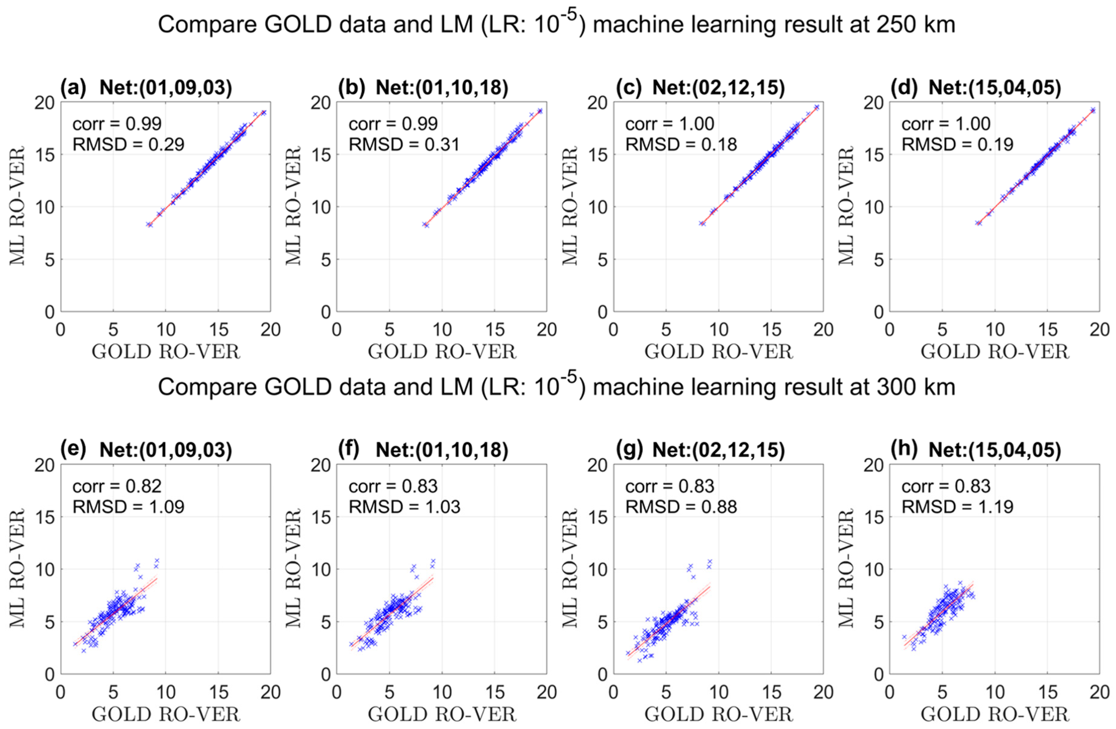
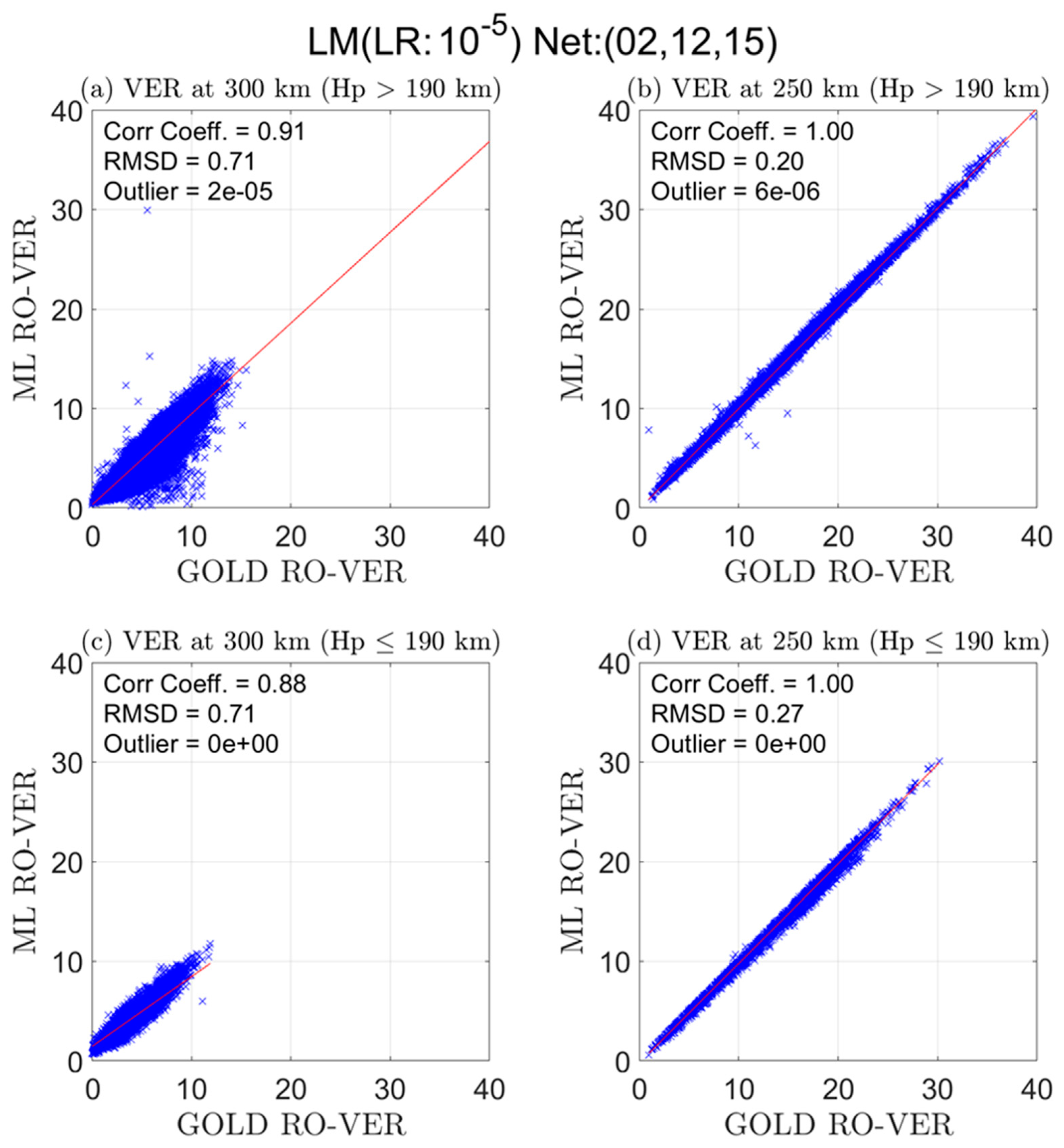
• LM: Levenberg-Marguardt (MATLAB: trainlm)
  The LM algorithm is the default setup of the feedforwardnet function in MATLAB, it is also known as the damped least-squares method, and can be viewed as a combination of the steepest descent method and the Gauss–Newton algorithm using a trust region approach. LM often converges faster than first-order methods, and it is used in many software applications for solving generic curve-fitting problems [31,32,33]. In short, LM is suitable for training small- and medium-sized problems, and the learning rate is better to be small if it is set as a constant [34].
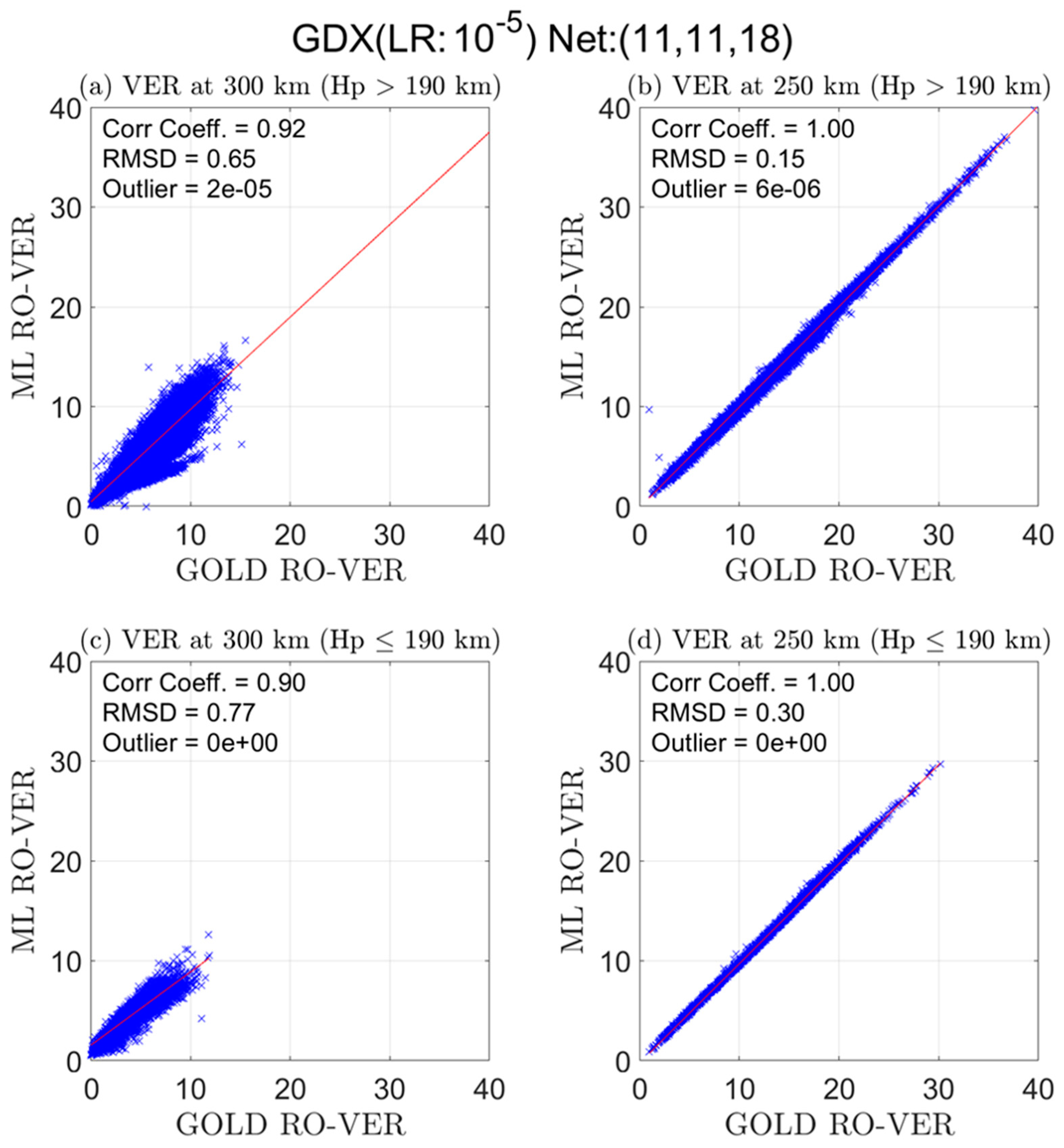
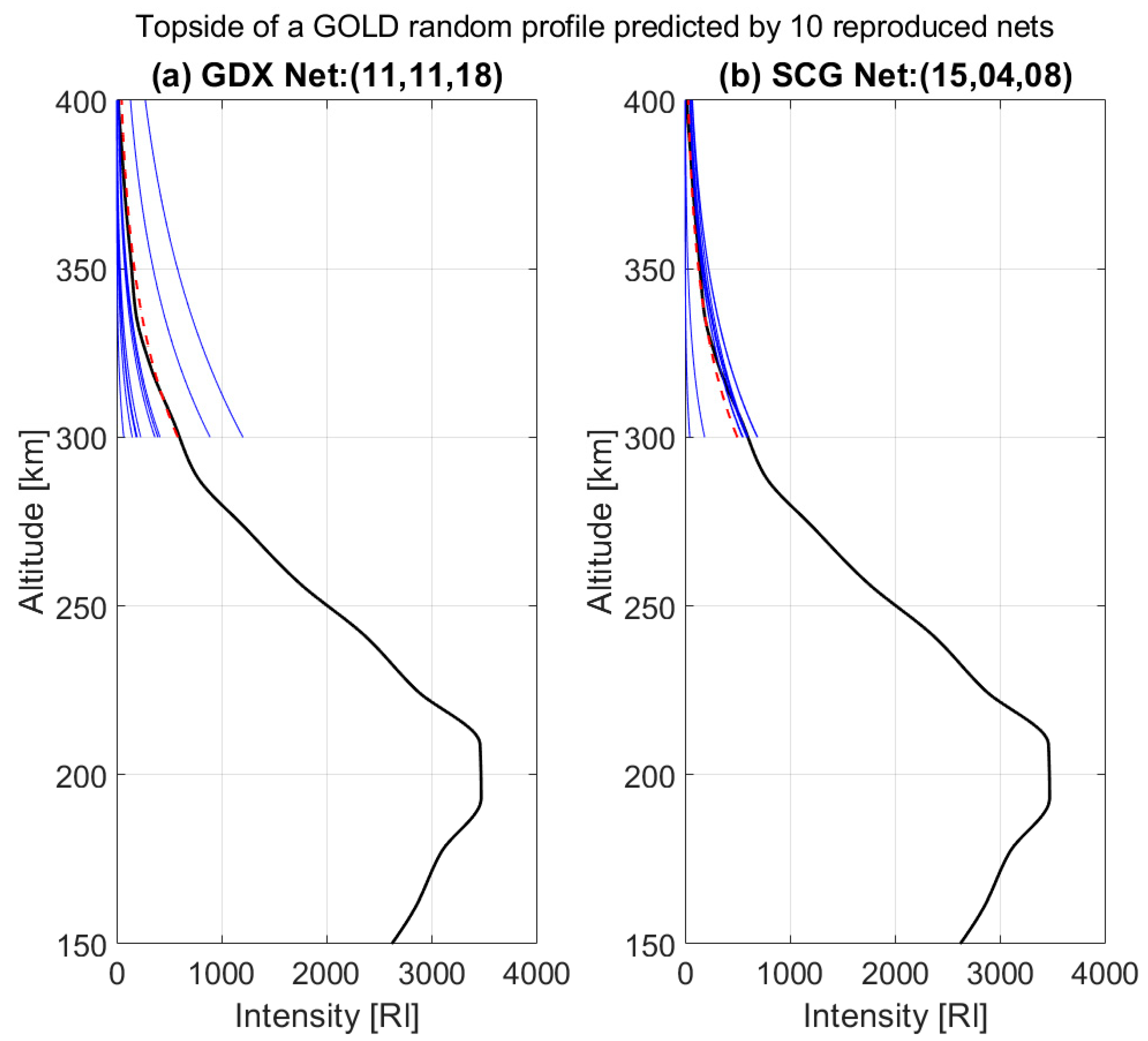
• GDX: Gradient descent with momentum and adaptive learning rate (MATLAB: traingdx)
  As one of the most popular algorithms to optimize neural networks, the gradient descent (GD) method is commonly used to minimize a cost function, which is a loss function that defines the performance of model prediction for a given set of parameters [35]. According to the equations derived by Ruder (2016) [35], GD obtains the next point from the gradient at the current position and scales it by a learning rate. By optimizing GD with Momentum, this application can solve the issue of the stagnant network resulting from the negligible cost function gradient at saddle points, and accelerate the process in the relevant direction like pushing a ball down a hill (Rauf Bhat, “Gradient Descent With Momentum”, Towards Data Science, 3 October 2020, accessed on 20 October 2022, https://towardsdatascience.com/gradient-descent-with-momentum-59420f626c8f). On the other hand, the learning rate can be considered the most influential hyperparameter in the training; however, choosing a proper learning rate is difficult due to the strong dependence, and the learning rate schedules are defined in advance and unable to adapt to the dataset’s characteristics (Manish Chablani, “Gradient descent algorithms and adaptive learning rate adjustment methods”, Towards Data Science, 14 July 2017, accessed on 20 October 2022, https://towardsdatascience.com/gradient-descent-algorithms-and-adaptive-learning-rate-adjustment-methods-79c701b086be.). The adaptive learning rate method is therefore applied to monitor and adjust learning rate in response for each of the weights in the model (Jason Brownlee, “How to configure the learning rate when training deep learning neural networks”, Deep Learning Performance, 23 January 2019, accessed on 20 October 2022, https://machinelearningmastery.com/learning-rate-for-deep-learning-neural-networks/). In this study, the ratios of increasing and decreasing learning rates are 1.05 and 0.7 as default, respectively.
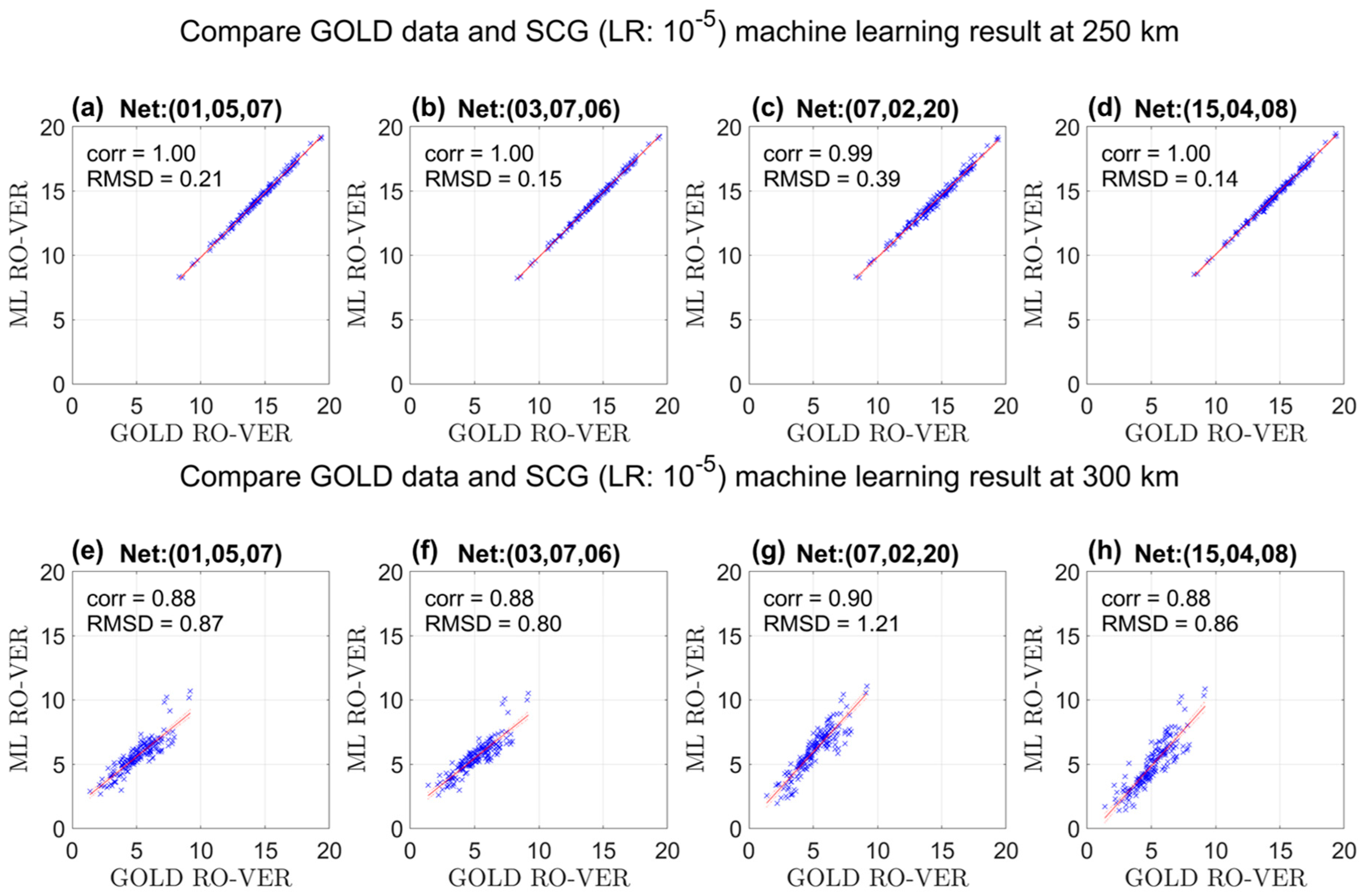
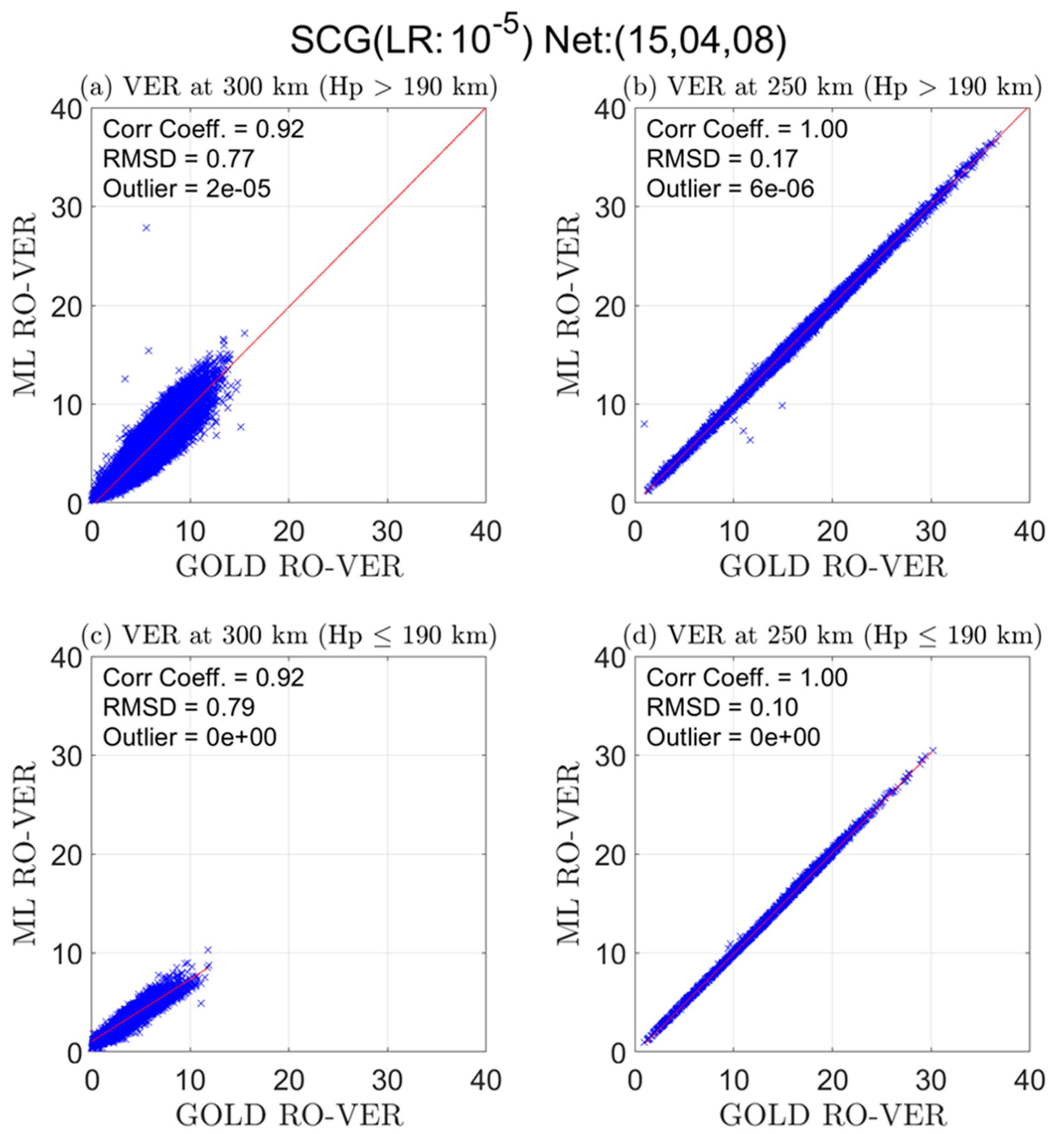
• SCG: Scaled conjugate gradient (MATLAB: trainscg)
  The conjugate gradient (CG) method is popular for solving large-scale nonlinear problems because it requires very low memory based on the simplicity of the iterations [36]. The scaled conjugate gradient (SCG) algorithm is designed to avoid the time-consuming line search based on conjugate directions [37]. The quadratic approximation of the error function defines the step size and increases the robustness and independency of user-defined parameters in the SCG training process. Notably, CG is recommended only for large problems due to its sensitivity to rounding errors (Albers Uzila, “Complete Step-by-step Conjugate Gradient Algorithm from Scratch”, Towards Data Science, 27 September 2021, accessed on 20 October 2022, https://medium.com/towards-data-science/complete-step-by-step-conjugate-gradient-algorithm-from-scratch-202c07fb52a8).

Furthermore, the input data are separated into 3 piles, the training and test sets are used for machine learning, while the validation set is used for checking the results and modifying the hyper-parameters during the learning process. The sets of training, test, and validation were divided randomly by 70:15:15 (%). During the training process, the transfer functions remain as the MATLAB default, Hyperbolic tangent sigmoid (tansig), for the hidden layers and Linear (purelin) for the output layer. The loss function is applied with the Mean Squared Error (MSE) regression to identify the performance. Subsequently, each algorithm has 8000 nets trained for meeting the same goal from this process, and only the well-performing ones remain for each to validate with GOLD limb data.

3.2. Abel Inversion

By comparing the VER derived from the original intensity profiles and the ones with the deep-learning constructed topside, the 8000 nets were validated and the well-performing nets were selected. In particular, one Rayleigh (R) is defined as a column emission rate of ${10}^6$$\mathrm{photons}·{\mathrm{cm}}^{-2}·{\mathrm{s}}^{-1}$ [38], and can be considered as a function of the tangent altitude (H). The position of the emission relative to the sensor is denoted as x in Equation (2), and $x_0$ and $x_1$ represent the positions of the sensor and the end of sight, respectively.

$$R\left(H\right)={\int }_{x_0}^{x_1}VER(x,H)·{10}^{-6}dx$$

(2)

Notably, since the airglow gradually becomes weaker with altitude, the end of the line of sight is considered as infinity here. One VER unit is defined as 1 $\mathrm{photons}·{\mathrm{cm}}^{-3}·{\mathrm{s}}^{-1}$, and can be considered as a function of x and H; hence, the physical meaning of $R\left(H\right)$ is the integration of VER along the horizontal line of sight of the sensor at the tangent point as shown in Figure 3.

In Figure 3, the geometry of transforming emission intensity into VER at the tangent point (VER${}_{TP}$) ) is demonstrated, and the retrieval is described in Equation (3). Based on the characteristics of light propagating along a straight line, the classical assumptions were made that the glow emission is spherically symmetric and evenly distributed on each shell. In other words, the horizontal variation of the VERs is excluded from the consideration. Equation (3) is similar to the radio occultation (RO) process of converting slant total electron content (STEC) into electron density (Ne) [39], except that the bending angle is considered as zero here.

$$VE{R}_{TP}\left(H_n\right)=\frac{R\left(H_n\right)-2·{\sum }_{i=1}^{n-1}VE{R}_{TP}\left(H_i\right)·l_{i,n}}{2·l_{n,n}}$$

(3)

When the line of sight cuts across through the ionospheric layers, the image captured by the satellite-based sensor is comprised of multiple rows of Rayleigh profiles. Each column of the Rayleigh profile is regarded as being from VER profiles integrated horizontally along the line of sight from the sensor to infinity, and the VERs on each spherical shell are considered the same. There were n grids for the altitude profile, and the distance between the sensor and the tangent point of the line of sight was denoted as l, while the other notations retain the same definition as in the equations mentioned previously. As demonstrated in Figure 3, each line of sight penetrates through the upper layer twice, and the VER${}_{TP}$ at $H_n$ was simply assumed to be the difference of $R\left(H_n\right)$ and the integration of the VER${}_{TP}$ above $H_n$. To be more specific, the application of Equation (3) began from the uppermost point to the bottommost point, and the height step was set to be 1 km. The uppermost nonzero intensity is considered to be equivalent to VER${}_{TP}$. Subsequently, the VER${}_{TP}$ retrieved by using different deep learning algorithm-trained topsides were compared from the VER${}_{TP}$ retrieved directly with GOLD limb 135.6 nm intensity profiles for advanced validation.

3.3. Photochemical Inversion Model

The photochemical reaction of the 135.6 nm emission is mainly triggered by the relative combination of an electron ($e^{-}$) and an atomic oxygen ion ($O^{+}$) as described in Equation (4) [40], and the ion-ion recombination between $O^{+}$ and $O^{-}$ with rate coefficients of each reaction denoted as $k_1,k_2,k_3$ in Equations (6)–(8) [41,42,43]. The $O^{*}$ and $h\nu$ in Equations (4)–(7) represent the excited atomic oxygen and the direct recombination photons, respectively.

$$O^{+}+e^{-}\stackrel{{\alpha }_1}{\to }{O}^{*}+h\nu$$

(4)

$$O{(}^5{S}_2)\to O{(}^{3}P)+h{\nu }_{135.6}$$

(5)

$$O+e^{-}\stackrel{k_1}{\to }{O}^{-}+h\nu$$

(6)

$$O^{-}+O^{+}\stackrel{k_2}{\to }{O}^{*}+O$$

(7)

$$O^{-}+O\stackrel{k_3}{\to }{O}_2+e^{-}$$

(8)

The photons emitted from the radiative recombination of $e^{-}$ and $O^{+}$ include the 135.6, 130.4, 102.7, 98.9, and 91.1 nm continuum as well as a variety of visible and infrared wavelengths, and the partial rate coefficient of the 135.6 nm emission yielding from radiative recombination (Equation (4)) is denoted as ${\alpha }_1$[44] here. The electric dipole intercombination transition results in the 135.6 nm emission as described in Equation (5). During the production of the $O^{*}$ as described in Equation (7), there are about 54% of $O^{*}$ releases 135.6 nm emission via the transition $O{(}^5{S}_2)\to O{(}^3{P}_{2,1})$, and the proportion of the $O^{*}$ is denoted as ${\beta }_{135.6}$. The rate coefficients are mainly adopted from Meléndez Alvira et al. (1999) [44] and listed in

Table 2. The rate coefficients for photochemical reactions of the 135.6 nm airglow emission [44,45].

Symbol	Value	Unit	Description
${\alpha }_1$	$7.3\times {10}^{-13}$	cm${}^3$s${}^{-1}$	Radiative recombination rate of the 135.6 nm emission (Equation (4)).
${\beta }_{135.6}$	0.54		Fraction of the 135.6 nm emission yielded by ion-ion recombination (Equation (9)).
$k_1$	$1.3\times {10}^{-15}$	cm${}^3$s${}^{-1}$	Production rate of $O^{-}$ (Equation (6)).
$k_2$	$1.0\times {10}^{-7}$	cm${}^3$s${}^{-1}$	Production rate of $O^{*}$ (Equation (7)).
$k_3$	$1.4\times {10}^{-10}$	cm${}^3$s${}^{-1}$	Loss rate of $O^{-}$ (Equation (8)).

. Accordingly, the VER of the 135.6 nm emission during nighttime is simply derived as Equation (9) based on the mechanism of the photochemical reactions [40,43].

$$VE{R}_{135.6}={\alpha }_1\left[O^{+}\right]\left[e^{-}\right]+\frac{{\beta }_{135.6}{k}_1{k}_2\left[O\right]\left[O^{+}\right]\left[e^{-}\right]}{k_2\left[O^{+}\right]+k_3\left[O\right]}$$

(9)

Since the [$O^{+}$] is widely known to be nearly identical to Ne in the $\mathit{F}$-region (Global-scale Observations of the Limb and Disk (GOLD), “Public Science Data Products Guide (Rev. 4.4)”, Documentation | NASA GOLD, 5 August 2022, accessed on 20 October 2022, https://gold.cs.ucf.edu/wp-content/documentation/GOLD_Public_Science_Data_Products_Guide_Rev4.4.pdf.), the Equation (10) was inverted from Equation (9) with the assumption of [$O^{+}$] ≈ Ne, and the Ne can be simplified as the positive real root of a cubic equation in one variable. Moreover, the NRLMSIS-00 empirical atmosphere model [46] is applied in this study to provide the [O] for inverting the 135.6 nm VER into Ne by using the Equation (10).

$$k_2{\alpha }_1{\left[e^{-}\right]}^3+(k_3{\alpha }_1\left[O\right]+{\beta }_{135.6}{k}_1{k}_2\left[O\right]){\left[e^{-}\right]}^2-VE{R}_{135.6}{k}_2\left[e^{-}\right]-VE{R}_{135.6}{k}_3\left[O\right]=0$$

(10)

With the techniques of deep learning, Abel inversion, and photochemical inversion model, we developed a procedure to optimize the RO-like retrieval of VER (referred to hereafter as RO-VER) under the condition of missing topside information and validated the performance with the GOLD limb 135.6 nm intensity observations in 2020.

4. Results

To estimate the inaccuracy of the RO-VER retrieved with machine learning (ML RO) predicted topside of intensity, it is essential to validate the performance of each net. To validate the similarity of the ML-derived VER topside profile to that derived using the actual GOLD observations, the GOLD observed 135.6 nm intensities in the region ≥ 300 km altitude were replaced by the net predicted intensities before retrieving VER profiles using the Abel inversion for the validations. In this section, there were two steps to select the top-performing nets from the 8,000 nets trained with LM, GDX, and SCG algorithms. The four top-performing nets of each algorithm were selected with quick filtering, and the best-performing net trained by each algorithm was hand-picked for reducing the inaccuracy of the RO-VER by subsequently applying the full collection of GOLD 135.6 nm limb data in 2020.

4.1. The Four Top-Performing Nets

First, we randomly subsampled a set of 320 profiles out of 387,900 nonzero profiles of GOLD limb 135.6 nm intensity profiles in 2020 for filtering the performance of the nets quickly. We selected four top-performing nets trained with each algorithm based on the correlation coefficient and root-mean-square deviation (RMSD, unit: VER) [47] between the GOLD RO-VER and ML RO-VER trained with the algorithms GDX, SCG, and LM at 250 km and 300 km as shown in Figure 4, Figure 5 and Figure 6. Figure 4 shows the scatter plots of GOLD RO-VER and ML RO-VER at 250 km (Figure 4a–d) and 300 km (Figure 4e–h) applied with four top-performing GDX nets. For the RO-VERs at 250 km, it is apparent that the correlation coefficients approach 1.0 due to the 135.6 nm intensities at 250 km being covered by GOLD observations, as opposed to being derived using ML.

Notably, the scatter diagrams of the GDX trained net with HDL ratio 8:15:12 (denoted as Net:(08, 15, 12)) at 300 km (Figure 4f) had the lowest correlation 0.91 and highest RMSD 1.48 VER among the four GDX nets at the same altitude (Figure 4e,g,h). Since the retrieval process of the Abel inversion begins from the uppermost point, the inaccuracy of the upper points has a significant influence on the retrieval at lower points. Therefore, despite the fact that the altitude at 250 km was included in the range of GOLD 135.6 nm observations, the blue scattering points of Net:(08, 15, 12) in Figure 4b showed the highest level of dispersion among the four GDX nets at 250 km, where the RMSD of the scatter was 0.55 VER.

Comparing to the correlations of the GOLD RO-VER and ML RO-VER at 300 km obtained from the top-performing nets trained with the GDX algorithm (Figure 4e–h), the same categories but trained with the SCG algorithm in Figure 5e–h can barely reach 0.9 at 300 km. Moreover, the highest correlation and lowest RMSD of the SCG training results at 250 km was the Net:(15, 04, 08) (Figure 5d). But for the SCG scatter diagrams at 300 km, the nets with the highest correlation and lowest RMSD are not the same net.

Similarly, Figure 6 shows the same categories but trained with the LM algorithm. The top four correlations of RO-VERs at 300 km obtained with the LM algorithm are the lowest among all machine learning algorithms applied in this study, with the correlation coefficients of RO-VERs at 300 km all less than 0.85. According to the comparisons in Figure 4, Figure 5 and Figure 6, it is quite intriguing how the number of neurons in a net can impact the performance of this application while the net was being trained by different algorithms. Subsequently, the number of nets with the specific number of total neurons and the correlation coefficients of RO-VERs at specific altitudes are compared in Figure 7.

Remarkably, the high correlation coefficients (≥0.9) of RO-VERs at 250 km (Figure 7a–c) are clustered the most when the number of total neurons in a net ranged from 20 to 45. The generally large correlations at 250 km of the nets were expected, due to the observed GOLD intensity dominating the results at 250 km, despite the inaccuracy impacted by the difference of GOLD limb 135.6 nm intensities and ML predicted intensities in the interval of the topside. On the other hand, since the ML RO-VERs at 300 km were simply based on ML prediction, it is reasonable that the correlation coefficients of RO-VERs at 300 km cannot approach 1.0 for most of the nets. Nevertheless, the nets trained with the GDX algorithm have general correlation coefficient values between 0.6–0.8 (Figure 7e). To briefly summarize the relationship between the total neuron number of each net and the correlation coefficient of RO-VERs, the analysis demonstrated in Figure 7 elucidates the better-performing combinations of total neuron numbers and algorithms for future use while setting up the training of similar applications.

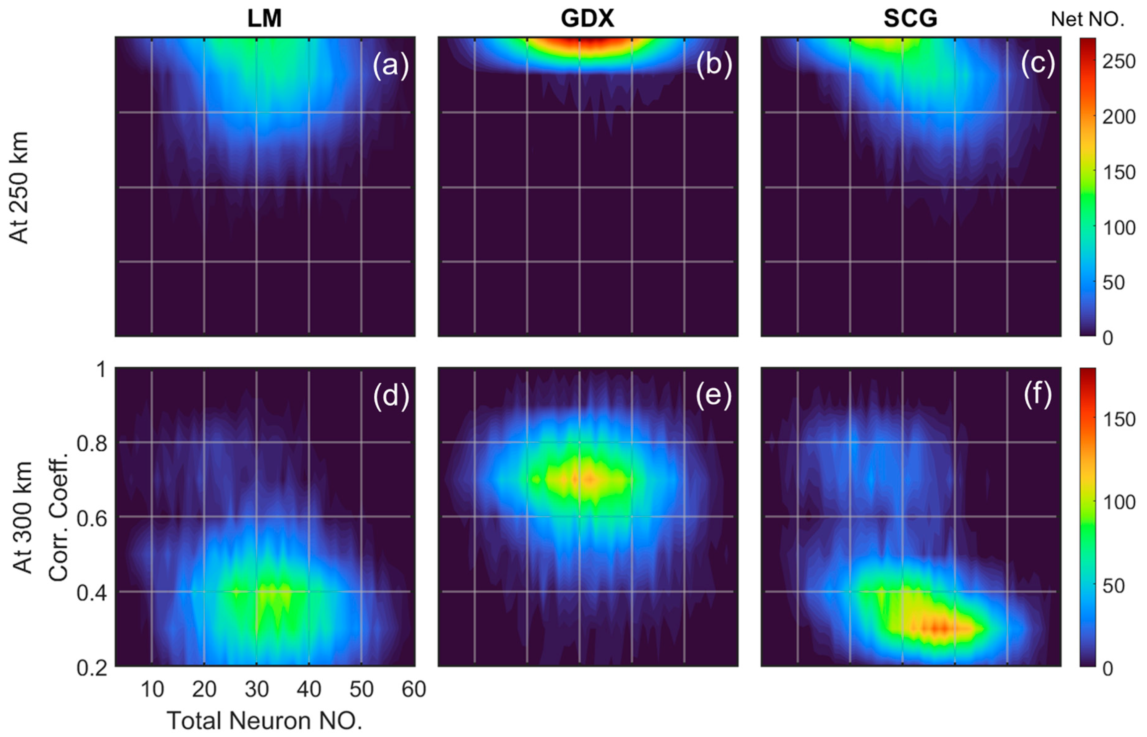
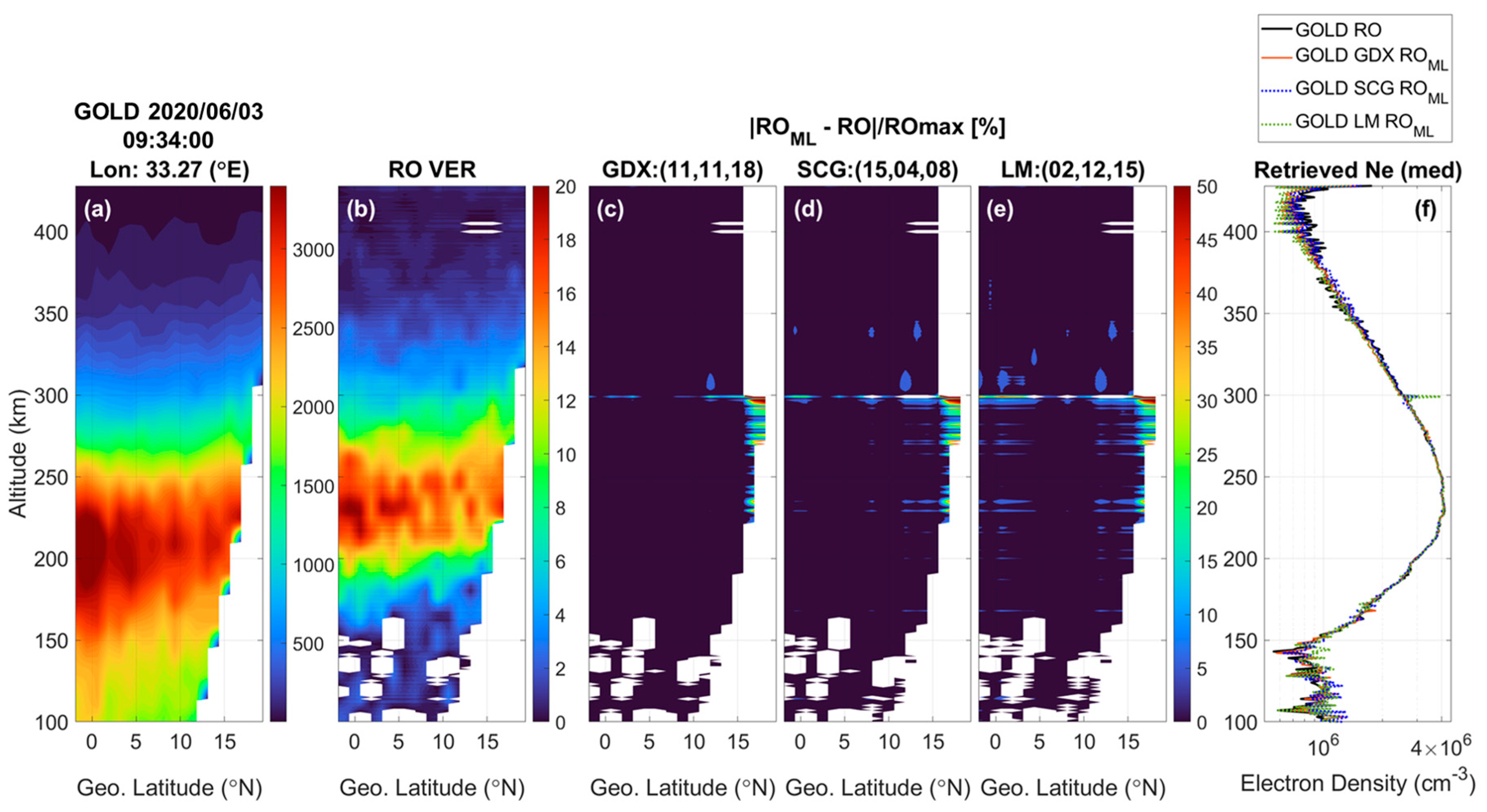
4.2. Best Net of Each Algorithm

Based on the results in the previous subsection, only one out of four top-performing nets for each algorithm will be selected for use in this stage. The full collection of GOLD limb 135.6 nm intensity data in 2020 was applied for detailed verification. Since most of the GOLD limb 135.6 nm $H_p$ in 2020 is above 190 km in altitude, and one of the given bottommost inputs to train the nets was defined to be at 180 km altitude (Figure 2), the scatter plots of RO-VERs at 250 km and 300 km altitude for each net in Figure 8, Figure 9 and Figure 10 were therefore divided into four groups to validate the applicability of nets above and below the assumed lowest $H_p$. Moreover, before obtaining correlation coefficients and RMSD, the negative RO-VERs and the ones larger than 2000 VER were classified as outliers and removed beforehand. In Figure 8, Figure 9 and Figure 10, the three nets trained by each algorithm (GDX, SCG, LM) have already been selected according to performance. Notably, the outlier proportions of the RO-VERs at 250 km and 300 km altitudes when the initial $H_p>$ 190 km altitude were identically $6.0\times {10}^{-6}$ and $2.0\times {10}^{-5}$ for all three nets (Figure 8a,b, Figure 9a,b and Figure 10a,b), and hence the outliers were excluded from the possibility of being caused by the nets.

The scatter plots of the GOLD RO-VERs and ML RO-VERs applied with the GDX algorithm trained Net:(11, 11, 18) are compared in Figure 8 based on the altitudes, and the four groups are RO-VERs at 300 km when $H_p>$ 190 km, at 250 km when $H_p>$ 190 km, at 300 km when $H_p\le$ 190 km, and at 250 km when $H_p\le$ 190 km. Besides the expected results of the near-perfect correlation of the RO-VERs at 250 km altitude (Figure 8b,c), the correlation coefficients of the RO-VERs at 300 km altitude are high (≥0.90) and the RMSDs are low (<1.0) regardless of whether the initial $H_p$ was greater than 190 km or not (Figure 8a,d).

Turning now to the best-performing net trained with the SCG algorithm, the scatter diagrams for verifying the SCG Net:(15, 04, 08) are shown in Figure 9. Similar to the case trained by the GDX algorithm, the correlation coefficients of RO-VERs at 250 km (Figure 9b,d) and 300 km (Figure 9a,c) altitudes in the case trained by the SCG algorithm were ideally high (≥0.90) as well.

Having demonstrated the hand-picked nets trained with GDX and SCG, the LM Net:(02, 12, 15) was then selected and verified in Figure 10. It is worth noting that although the correlation coefficients of RO-VERs at 250 km altitude in the case trained by the LM algorithm (Figure 10b,d) were equal to 1.0, the RMSDs here were the largest compared to the same categories of GDX (Figure 8b,d) and SCG (Figure 9b,d) at the same altitude. In addition, Figure 10a illustrates that there is a small cluster of underestimated ML RO-VERs at 300 km altitude when the initial intensity $H_p$ is above 190 km altitude, and the RO-VERs dispersed the most in the case of LM among all algorithms applied in this study at both 250 km and 300 km altitudes. As for the RO-VERs at 300 km altitude but with the initial intensity $H_p$ below the 190 km altitude (Figure 10c), the correlation coefficient between GOLD and ML RO-VERs is 0.88, which is the lowest among Figure 8, Figure 9 and Figure 10 as well.

So far the three hand-picked deep learning nets trained with each algorithm have been verified and compared, and are summarized in

Table 3. Comparison of the performance of the nets trained with three different algorithms (GDX, SCG, LM) according to the correlation coefficients and RMSDs between GOLD RO-VERs and ML RO-VERs.

	GDX	SCG	LM
Number of Nets Above Threshold *	250	92	28
Training Speed Ranking	1	2	3
Overall Ranking	1	2	3
Selected Net	(11, 11, 18)	(15, 04, 08)	(02, 12, 15)

* The threshold criteria were set as correlation coefficient ≥ 0.9 at 250 km altitude, and ≥0.8 at 300 km altitude.

. First, the number of nets above the threshold for each algorithm is compared, and the threshold criteria were set when the correlation coefficient between GOLD and ML RO-VER is greater than 0.9 at 250 km altitude, and greater than 0.8 at 300 km altitude.

According to the given criteria, the outcomes of GDX had the largest number meeting the criteria, as 250 nets were found to meet the interval of correlation coefficients. The outcomes of LM had the fewest, with only 28 nets meeting the criteria. On the other hand, the training speed is an important parameter to learn from this experiment as well, and the ranking was made under the same host environment and conditions. There were 8000 loops for each algorithm in this application, and the GDX nets were trained fastest amongst all algorithms. The overall performance of each algorithm can be distinguished according to the results illustrated in Figure 4, Figure 5, Figure 6, Figure 7, Figure 8, Figure 9 and Figure 10, and so far the order of usability to our application was GDX > SCG > LM. Notably, the overall ranking made in this study might be different if the hyperparameters of the training are tuned in a different way, or when this method is applied to a different type of data.

Based on the scatter diagrams in Figure 8, Figure 9 and Figure 10, the RMSDs of RO-VERs were smaller than 1.0 VER at both 250 km and 300 km altitudes. What follows is one example of our application in this study applied to a single instance of GOLD observed 135.6 nm emissions on 3 June 2022 at 09:34 UT (Figure 11). By using the photochemical inversion model and empirical models IRI-2016 [48] and NRLMSISE-00 [46], the inverted Ne deviation at 300 km resulted from only 1 $\Delta$VER difference ranges in (1.0–6.5)$\times {10}^5{\mathrm{cm}}^{-3}$ approximately according to Equation (10). In Figure 11, the GOLD 135.6 nm intensity profiles (Figure 11a) were first retrieved into GOLD RO-VER profiles (Figure 11b). After that, the difference between GOLD RO-VERs and ML RO-VERs of GDX Net:(11, 11, 18), SCG Net:(15, 04, 08), and LM Net:(02, 12, 15) were compared (Figure 11c–e). Lastly, the median Ne profiles inverted from the GOLD RO-VER and ML RO-VER of each net were plotted to evaluate the inaccuracy resulting from the prediction of each net (Figure 11f).

In particular, the discrepancy between GOLD RO-VER and ML RO-VER was calculated as a percentage of the GOLD RO-VER maximum ($R{O}_{max}$) of each profile. The formula was given as $|R{O}_{ML}-RO|/R{O}_{max}$, where $R{O}_{ML}$ denoted ML RO-VER, and $RO$ denoted GOLD RO-VER. It can be seen that GDX Net: (11, 11, 18) generally had the fewest discrepancies among Figure 11c–e, and the discrepancies were mostly less than 5% except for the anomalies at the boundary on the right-hand side. In Figure 11f, it is shown that the median Ne inverted from ML RO-VERs of the GDX Net: (11, 11, 18) and SCG Net: (15, 04, 08) in the interval ranging from 180 km to 320 km altitude can show good consistency with the one inverted from GOLD RO-VERs ideally. On the contrary, the median Ne inverted from ML RO-VERs of the LM Net: (02, 12, 15) was found to have a large discrepancy with the one inverted from GOLD RO-VERs at 300 km altitude.

However, Figure 11 only showed one example of a single instance for the RO retrieval and Ne inversion. Although the other cases were not shown as Figures in this study, it was clear that GDX Net: (11, 11, 18) and SCG Net: (15, 04, 08) performed better than LM Net: (02, 12, 15) in the most cases. The GDX Net: (11, 11, 18) was not always the best-performing net, sometimes the SCG Net: (15, 04, 08) performs better than the GDX Net: (11, 11, 18). In addition, it is important to ask how to train the best-performing net efficiently in the fewest number of trials. Take the GDX Net: (11, 11, 18) as an example, it remains a question as to whether it is possible to train an identical net to this one with the same initial hyperparameters and setup. To verify the possibility of reproducing the same GDX Net: (11, 11, 18) directly, we independently reproduced the net 10 times with HDLs set as (11, 11, 18), and trained these nets with the GDX algorithm, without changing any other initial setup parameters. The same was done with the 10 reproduced nets of the SCG Net: (15, 04, 08). Subsequently, a random GOLD 135.6 nm intensity profile was applied here to confirm the performance of the 10 reproduced nets of each algorithm. The topsides of this random intensity profile predicted by the nets are shown in Figure 12.

The black solid line in Figure 12 indicates the randomly selected GOLD 135.6 nm limb intensity profile, and the red dashed line in Figure 12a denotes the topside of the profile predicted by the GDX Net: (11, 11, 18) generated in the 8000 training loops, while the one predicted by the SCG Net: (15, 04, 08) was denoted in Figure 12b. Remarkably, the GDX Net: (11, 11, 18) predicted topside (red) matched the GOLD intensity profile (black) ideally, and the difference of the intensities at 300 km altitude was extremely small. Nevertheless, the topsides in blue predicted by the reproduced nets did not perform as well as the original GDX Net: (11, 11, 18).

Two items could be suggested as the cause of the training uncertainty, which are the adaptive learning rate and the activation level of each neuron. The setting of the adaptive learning rate can automatically customize the learning rate continuously according to the varying gradient, and the activated level of each neuron is also defined automatically during the process. On the other hand, the SCG Net: (15, 04, 08) was trained with a fixed learning rate instead an adaptive one, and most of the reproduced nets (blue) with HDLs set as 15:4:8 have similar performance as the one generated from 8000 training loops, with some even perform better than the original one. However, the main hyperparameters that dominate the uncertainty of the training remain a topic for further studies and more validations in the future.

5. Discussions

This study aimed to develop a method to optimize the quality of Abel inversion by applying the technique of machine learning while retrieving profiles with a given uppermost value that does not converge to zero (Figure 2), such as the FORMOSAT-2/ISUAL observed 630.0 nm intensities that were only collected below 300 km altitude (Figure 1). In the first stage of the validation, the four top-performing nets trained by GDX, SCG, and LM and each generated from 8000 loops were selected based on the scatter diagrams of the net-predicted results and the 320 random GOLD RO-VERs at 250 km and 300 km altitudes (Figure 4, Figure 5 and Figure 6). Comparing the relevance of RO-VERs in the cases of different training algorithms, the GDX nets have the best performance among all algorithms that the correlation coefficients of the RO-VERs at 300 km altitude are within 0.6–0.8 mostly (Figure 7e), and there are 250 GDX nets found to meet the high correlation threshold criteria defined in this study (Table 3). Moreover, the GDX and SCG algorithms train much faster than the LM algorithm does when the initial learning rate is set as ${10}^{-5}$ in terms of the time spent on looping 8000 times to search for well-performing nets.

The best-performing net of each algorithm was then verified with the full collection of the GOLD 135.6 nm intensity profiles in 2020 and selected according to correlation coefficient thresholds at 250 and 300 km altitude. The selected nets were GDX Net: (11, 11, 18), SCG Net: (15, 04, 08), and LM Net: (02, 12, 15). The scatter diagrams of RO-VERs when the $H_p$ of the intensity profile before applying Abel inversion was above and below 190 km altitude were compared for each best-performing net to validate the usability of the nets (Figure 8, Figure 9 and Figure 10). Furthermore, the correlation coefficients of RO-VERs at 300 km altitude when $H_p$ is below 190 km altitude are all larger than 0.85 for the three hand-picked nets. Regarding the relevance of RO-VERs when initial intensity $H_p$ is above or below the bottommost altitude set for the given inputs of training, there existed some nets (not shown in this study) found to have high correlation coefficients (≥0.9) of RO-VERs when the initial $H_p$ was above 190 km altitude, but the GOLD RO-VERs and ML RO-VERs were barely relevant to each other when the initial $H_p$ was below 190 km altitude. This finding revealed the fact that the bottommost altitude set for given inputs plays an essential role in the training, and a general scatter diagram including the RO-VERs retrieved from intensity profiles with its $H_p$ in every interval is not enough to validate and distinguish the quality of the nets. Moreover, the experiment went a step further to the invert Ne from the RO-VERs by finding the positive real root for the photochemical inversion model of the 135.6 nm airglow emission (Equation (10)), and the NRLMSISE-00 empirical atmosphere model generated [O] results were applied for this inversion. It was found that 1 $\Delta$VER difference can result in an inaccuracy of approximately (1.0–6.5) $\times {10}^5{\mathrm{cm}}^{-3}$ while inverting into Ne by applying the photochemical inversion model, and the absolute differences of GOLD RO-VERs and ML RO-VERs of GDX and SCG divided by the GOLD RO-VER maximum were verified to be less than 5% generally except for the anomalies at the limb boundary (Figure 11), which demonstrates that the inaccuracy resulting from the Abel inversion can be significantly reduced by applying the well-trained deep learning GDX and SCG nets. On the contrary, it took an extremely long period to complete the 8,000-loop training with the LM algorithm when the learning rate was set as ${10}^{-5}$ in our application, while the nets that can meet the high-performance threshold are the fewest amongst the three algorithms. Therefore, the LM algorithm is not recommended for this type of application accordingly.

It remains a question still as to how to reproduce an identical net to the one generated from the 8,000 loops. There are many hyperparameters defined automatically that may increase the variability while reproducing the nets with the same HDLs setup, such as the adaptive learning rate and the activation level of each neuron. Although the generation of a well-performing net is found to be easier through training with the GDX algorithm when the total amount of neurons is set to be within 20 to 45 approximately compared to SCG and LM, GDX becomes an algorithm that is more unstable to train with while reproducing nets with the same amount of neurons in every layer due to the adaptive learning rate setup (Figure 12a). Conversely, a well-performing net could be reproduced more easily by applying the SCG algorithm with a specific HDLs setup (Figure 12b). However, there remain other hyperparameters that dominate the variability of the training process, so the reproduced nets will still not be exactly the same. In short, this study developed a method to train neural networks for optimizing the Abel inversion when the uppermost value of a profile does not converge to zero. A perspective on the level of difficulty to reproduce the well-performing nets proposed in this research by training with different algorithms were provided as well.

6. Conclusions

In conclusion, a methodology is developed in this research for retrieving VER from limb-viewed airglow emission intensity using the techniques of Abel inversion and machine learning. It has the potential to aid in the long-term analysis of the ionosphere by resolving past data with incomplete limb-viewed intensity profiles. The use of well-performing neural networks, generated using the three algorithms (GDX, SCG, LM), demonstrated the effectiveness of this method in improving the accuracy of vertical ionospheric profiles, and was validated using a large number of GOLD limb-viewed 135.6 nm intensity profiles. It was found that the GDX algorithm had the highest probability of generating high-performing networks when the number of neurons ranged from 20 to 45, while the LM algorithm was the least effective. Additionally, it was observed that the SCG algorithm resulted in neural networks that were more easily reproduced to have similar performance compared to those trained with the GDX algorithm. However, further study is needed to understand the specific hyper-parameters that contribute to the variability of training outcomes and improve the stability of the network reproducing process. Additionally, the effectiveness of other machine learning algorithms should be explored in future research. Overall, the combination of Abel inversion and machine learning techniques presented in this research holds promise for advancing our understanding of the large-scale variations of the ionosphere with intensity data.

References

1. Yue, X.; Schreiner, W.S.; Rocken, C.; Kuo, Y.H. Evaluation of the orbit altitude electron density estimation and its effect on the Abel inversion from radio occultation measurements. Radio Sci. 2011, 46, 1–10. [Google Scholar] [CrossRef] [Green Version]
2. Wee, T.K. A variational regularization of Abel transform for GPS radio occultation. Atmos. Meas. Tech. 2018, 11, 1947–1969. [Google Scholar] [CrossRef] [Green Version]
3. Ogawa, T.; Balan, N.; Otsuka, Y.; Shiokawa, K.; Ihara, C.; Shimomai, T.; Saito, A. Observations and modeling of 630 nm airglow and total electron content associated with traveling ionospheric disturbances over Shigaraki, Japan. EPS 2002, 54, 45–56. [Google Scholar] [CrossRef] [Green Version]
4. Khomich, V.; Semenov, A.; Shefov, N. Airglow as an Indicator of Upper Atmospheric Structure and Dynamics; Springer Science and Business Media: New York, NY, USA, 2008. [Google Scholar] [CrossRef]
5. Meneses, F.; Muralikrishna, P.; Clemesha, B. Height profiles of OI 630 nm and OI 557.7 nm airglow intensities measured via rocket-borne photometers and estimated using electron density data: A comparison. Geofis. Int. 2008, 47, 161–166. [Google Scholar] [CrossRef]
6. Rajesh, P.K.; Liu, J.Y.; Hsu, M.L.; Lin, C.H.; Oyama, K.I.; Paxton, L.J. Ionospheric electron content and NmF2 from nighttime OI 135.6 nm intensity. J. Geophys. Res. 2011, 116. [Google Scholar] [CrossRef]
7. Vimal, S. Long-Term Changes in Night Time Airglow Emission at 557.7 nm over Mid Latitude Japanese Station i.e., Kiso (35.79° N, 137.63° E). Am. J. Clim. Chang. 2012, 1, 210–216. [Google Scholar] [CrossRef] [Green Version]
8. Mende, S.B.; Frey, H.U.; Rider, K.; Chou, C.; Harris, S.E.; Siegmund, O.H.W.; England, S.L.; Wilkins, C.; Craig, W.; Immel, T.J.; et al. The Far Ultra-Violet Imager on the Icon Mission. Space Sci. Rev. 2017, 212, 655–696. [Google Scholar] [CrossRef] [Green Version]
9. Laskar, F.I.; Eastes, R.W.; Martinis, C.R.; Daniell, R.E.; Pedatella, N.M.; Burns, A.G.; McClintock, W.; Goncharenko, L.P.; Coster, A.; Milla, M.A.; et al. Early Morning Equatorial Ionization Anomaly From GOLD Observations. J. Geophys. Res. 2020, 125, e2019JA027487. [Google Scholar] [CrossRef]
10. Cai, X.; Burns, A.G.; Wang, W.; Qian, L.; Liu, J.; Solomon, S.C.; Eastes, R.W.; Daniell, R.E.; Martinis, C.R.; McClintock, W.E.; et al. Observation of Postsunset OI 135.6 nm Radiance Enhancement Over South America by the GOLD Mission. J. Geophys. Res. 2021, 126, e2020JA028108. [Google Scholar] [CrossRef]
11. Rodríguez-Zuluaga, J.; Stolle, C.; Yamazaki, Y.; Xiong, C.; England, S.L. A Synoptic Scale Wavelike Structure in the Nighttime Equatorial Ionization Anomaly. Earth Space Sci. 2021, 8, e01529. [Google Scholar] [CrossRef]
12. Tam, S.W.Y.; Chiang, C.Y.; Huang, K.C.; Chang, T.F. Retrieval of Airglow Emission Rates in Analytical Form for Limb-Viewing Satellite Observations at Low Latitudes. J. Geophys. Res. 2021, 126, e2021JA029490. [Google Scholar] [CrossRef]
13. Murphy, K. Machine Learning: A Probabilistic Perspective; Adaptive Computation and Machine Learning Series; MIT Press: Cambridge, MA, USA, 2012. [Google Scholar]
14. Sai Gowtam, V.; Tulasi Ram, S. An Artificial Neural Network-Based Ionospheric Model to Predict NmF2 and hmF2 Using Long-Term Data Set of FORMOSAT-3/COSMIC Radio Occultation Observations: Preliminary Results. J. Geophys. Res. 2017, 122, 11743–11755. [Google Scholar] [CrossRef]
15. Thandlam, V.; Venkatramana, K. Enhancing Vertical Resolution of Satellite Atmospheric Profile Data: A Machine Learning Approach. Int. J. Adv. Res. 2018, 6, 542–550. [Google Scholar] [CrossRef] [Green Version]
16. Xiao, Z.; Wang, J.; Li, J.; Zhao, B.; Hu, L.; Liu, L. Deep-learning for ionogram automatic scaling. Adv. Space Res. 2020, 66, 942–950. [Google Scholar] [CrossRef]
17. Hsieh, M.C.; Huang, G.H.; Dmitriev, A.V.; Lin, C.H. Deep Learning Application for Classification of Ionospheric Height Profiles Measured by Radio Occultation Technique. Remote Sens. 2022, 14, 4521. [Google Scholar] [CrossRef]
18. Rajesh, P.K.; Chen, C.H.; Lin, C.H.; Liu, J.Y.; Huba, J.D.; Chen, A.B.; Hsu, R.R.; Chen, Y.T. Low-latitude midnight brightness in 630.0 nm limb observations by FORMOSAT-2/ISUAL. J. Geophys. Res. 2014, 119, 4894–4904. [Google Scholar] [CrossRef]
19. Eastes, R.W.; McClintock, W.E.; Burns, A.G.; Anderson, D.N.; Andersson, L.; Aryal, S.; Budzien, S.A.; Cai, X.; Codrescu, M.V.; Correira, J.T.; et al. Initial Observations by the GOLD Mission. J. Geophys. Res. 2020, 125, e27823. [Google Scholar] [CrossRef]
20. Solomon, S.C.; Andersson, L.; Burns, A.G.; Eastes, R.W.; Martinis, C.; McClintock, W.E.; Richmond, A.D. Global-Scale Observations and Modeling of Far-Ultraviolet Airglow During Twilight. J. Geophys. Res. 2020, 125, e2019JA027645. [Google Scholar] [CrossRef] [Green Version]
21. McClintock, W.E.; Eastes, R.W.; Hoskins, A.C.; Siegmund, O.H.W.; McPhate, J.B.; Krywonos, A.; Solomon, S.C.; Burns, A.G. Global-Scale Observations of the Limb and Disk Mission Implementation: 1. Instrument Design and Early Flight Performance. J. Geophys. Res. 2020, 125, e2020JA027797. [Google Scholar] [CrossRef]
22. McClintock, W.E.; Eastes, R.W.; Beland, S.; Bryant, K.B.; Burns, A.G.; Correira, J.; Danielll, R.E.; Evans, J.S.; Harper, C.S.; Karan, D.K.; et al. Global-Scale Observations of the Limb and Disk Mission Implementation: 2. Observations, Data Pipeline, and Level 1 Data Products. J. Geophys. Res. 2020, 125, e2020JA027809. [Google Scholar] [CrossRef]
23. Titheridge, J.E. Ionogram analysis: Least squares fitting of a Chapman-layer peak. Radio Sci. 1985, 20, 247–256. [Google Scholar] [CrossRef]
24. Chapman, S. The absorption and dissociative or ionizing effect of monochromatic radiation in an atmosphere on a rotating earth part II. Grazing incidence. Proc. Phys. Soc. 1931, 43, 483–501. [Google Scholar] [CrossRef]
25. Chapman, S. Note on the Grazing-Incidence Integral Ch(X,χ) for Monochromatic Absorption in an Exponential Atmosphere. Proc. Phys. Soc. Sect. B 1953, 66, 710–712. [Google Scholar] [CrossRef]
26. Lagos, P.; Bellew, W.; Silverman, S.M. The airglow 6300 [OI] emission theoretical considerations on the luminosity profile. J. Atmos. Terr. Phys. 1963, 25, 581–587. [Google Scholar] [CrossRef]
27. Hargreaves, J.K. The Solar-Terrestrial Environment; Cambridge Univ. Press: New York, NY, USA, 1992. [Google Scholar]
28. Stankov, S.M.; Jakowski, N.; Heise, S.; Muhtarov, P.; Kutiev, I.; Warnant, R. A new method for reconstruction of the vertical electron density distribution in the upper ionosphere and plasmasphere. J. Geophys. Res. 2003, 108, 1164. [Google Scholar] [CrossRef]
29. Kil, H.; Lee, W.K.; Shim, J.; Paxton, L.J.; Zhang, Y. The effect of the 135.6 nm emission originated from the ionosphere on the TIMED/GUVI O/N2 ratio. J. Geophys. Res. 2013, 118, 859–865. [Google Scholar] [CrossRef]
30. Cai, X.; Burns, A.G.; Wang, W.; Coster, A.; Qian, L.; Liu, J.; Solomon, S.C.; Eastes, R.W.; Daniell, R.E.; McClintock, W.E. Comparison of GOLD Nighttime Measurements With Total Electron Content: Preliminary Results. J. Geophy. Res. 2020, 125, e2019JA027767. [Google Scholar] [CrossRef]
31. Wilamowski, B.M.; Yu, H. Improved Computation for Levenberg–Marquardt Training. IEEE Trans. Neural Netw. 2010, 21, 930–937. [Google Scholar] [CrossRef]
32. Transtrum, M.K.; Sethna, J.P. Improvements to the Levenberg-Marquardt algorithm for nonlinear least-squares minimization. arXiv 2012, arXiv:1201.5885. [Google Scholar] [CrossRef]
33. Gavin, H.P. The Levenberg-Marquardt Algorithm for Nonlinear Least Squares Curve-Fitting Problems; Duke University: Durham, NC, USA, 2019; Volume 19. [Google Scholar]
34. Yu, H.; Wilamowski, B.M. Intelligent Systems: Levenberg-Marquardt Training; CRC Press: Boca Raton, FL, USA, 2018; pp. 1–16. [Google Scholar] [CrossRef]
35. Ruder, S. An overview of gradient descent optimization algorithms. arXiv 2016, arXiv:1609.04747. [Google Scholar]
36. Yao, S.; Lu, X.; Wei, Z. A Conjugate Gradient Method with Global Convergence for Large-Scale Unconstrained Optimization Problems. J. Appl. Math. 2013, 2013, 730454. [Google Scholar] [CrossRef] [Green Version]
37. Babani, L.; Jadhav, S.; Chaudhari, B. Scaled Conjugate Gradient Based Adaptive ANN Control for SVM-DTC Induction Motor Drive. In Proceedings of the Artificial Intelligence Applications and Innovations, Thessaloniki, Greece, 16–18 September 2016; Iliadis, L., Maglogiannis, I., Eds.; IFIP Advances in Information and Communication Technology; Springer: Berlin/Heidelberg, Germany, 2016; Volume 475, pp. 384–395. [Google Scholar] [CrossRef] [Green Version]
38. Baker, D.J.; Romick, G.J. The rayleigh: Interpretation of the unit in terms of column emissionrate or apparent radiance expressed in SI units. Appl. Opt. 1976, 15, 1966–1968. [Google Scholar] [CrossRef]
39. Lin, C.Y.; Lin, C.C.H.; Liu, J.Y.; Rajesh, P.K.; Matsuo, T.; Chou, M.Y.; Tsai, H.F.; Yeh, W.H. The Early Results and Validation of FORMOSAT-7/COSMIC-2 Space Weather Products: Global Ionospheric Specification and Ne-Aided Abel Electron Density Profile. J. Geophys. Res. 2020, 125, e2020JA028028. [Google Scholar] [CrossRef]
40. Hanson, W.B. Radiative recombination of atomic oxygen ions in the nighttime F region. J. Geophys. Res. 1969, 74, 3720–3722. [Google Scholar] [CrossRef]
41. Knudsen, W.C. Tropical ultraviolet nightglow from oxygen ion-ion neutralization. J. Geophys. Res. 1970, 75, 3862. [Google Scholar] [CrossRef]
42. Hanson, W.B. A comparison of the oxygen ion-ion neutralization and radiative recombination mechanisms for producing the ultraviolet nightglow. J. Geophys. Res. 1970, 75, 4343–4346. [Google Scholar] [CrossRef]
43. Tinsley, B.A.; Christensen, A.B.; Bittencourt, J.; Gouveia, H.; Angreji, P.D.; Takahashi, H. Excitation of oxygen permitted line emissions in the tropical nightglow. J. Geophys. Res. 1973, 78, 1174–1186. [Google Scholar] [CrossRef] [Green Version]
44. Meléndez-Alvira, D.J.; Meier, R.R.; Picone, J.M.; Feldman, P.D.; McLaughlin, B.M. Analysis of the oxygen nightglow measured by the Hopkins Ultraviolet Telescope: Implications for ionospheric partial radiative recombination rate coefficients. J. Geophys. Res. 1999, 47, 14901–14913. [Google Scholar] [CrossRef]
45. Qin, J.; Makela, J.J.; Kamalabadi, F.; Meier, R.R. Radiative transfer modeling of the OI 135.6 nm emission in the nighttime ionosphere. J. Geophys. Res. 2015, 120, 10116–10135. [Google Scholar] [CrossRef]
46. Picone, J.M.; Hedin, A.E.; Drob, D.P.; Aikin, A.C. NRLMSISE-00 empirical model of the atmosphere: Statistical comparisons and scientific issues. J. Geophys. Res. 2002, 107, SIA 15-1–SIA 15-16. [Google Scholar] [CrossRef]
47. Hyndman, R.J.; Koehler, A.B. Another look at measures of forecast accuracy. Int. J. Forecast. 2006, 22, 679–688. [Google Scholar] [CrossRef] [Green Version]
48. Bilitza, D.; Altadill, D.; Truhlik, V.; Shubin, V.; Galkin, I.; Reinisch, B.; Huang, X. International Reference Ionosphere 2016: From ionospheric climate to real-time weather predictions. Space Weather 2017, 15, 418–429. [Google Scholar] [CrossRef]
49. Eastes, R.W.; Solomon, S.C.; Daniell, R.E.; Anderson, D.N.; Burns, A.G.; England, S.L.; Martinis, C.R.; McClintock, W.E. Global-Scale Observations of the Equatorial Ionization Anomaly. Geophys. Res. Lett. 2019, 46, 9318–9326. [Google Scholar] [CrossRef]
Figure 1. The FORMOSAT–2/ISUAL captured 630.0 nm airglow emission intensity (unit: Rayleighs) on 25 February 2009 at 16:26:42 Universal time. (a) The ECEF position of FORMOSAT-2 (red star) and the image (contour). (b) The 630.0 nm emission intensity is within 50–300 km. The vertical and horizontal axes indicate the tangent altitude and geographic latitude (°N), respectively.
Atmosphere 14 00074 g001
Figure 2. Illustration of deep learning training method. The left panel shows a profile of intensity as an example, while the middle panel demonstrates the input, hidden, and output layers of the artificial neural network. The partial Chapman distribution of the type coefficient (c) as 1, and thickness ( σ ) as 38 km is in red, and the blue part indicates the observed Rayleigh. The right diagram shows an OSSE result, the maximum absolute difference of the model-derived VER (considered as ground truth data in OSSE), and the Abel retrieved VER in this case within 150–280 km with different sets of (c, σ ). The altitude of the peak intensity ( R p ) is denoted as H p , and the ratio of intensities at 290 km ( R 1 / R p ), 280 km ( R 2 / R p ), and 180 km ( R 3 / R p ) are selected as inputs. There are 3 hidden layers, and the outputs are c and σ .
Atmosphere 14 00074 g002
Figure 3. Geometry of the Abel inversion for transforming emission intensity (Rayleigh) into VER at the tangent point.
Atmosphere 14 00074 g003
Figure 4. Scatter plots of the four top-performing nets trained with GDX algorithm in the comparison of RO-VER at (ad) 250 km and (eh) 300 km between randomly subsampled 320 profiles of VERs retrieved from GOLD limb intensity (GOLD RO-VER) and machine learning topside profiles (ML RO-VER). The linear regression is indicated as a red solid line. The correlation coefficient and root-mean-square deviation (RMSD, unit: VER) of each scatter diagram are noted on the top left of each subplot. From left to right, the nets with the number of neurons in three hidden layers (HDL) are (03, 11, 13), (08, 15, 12), (11, 11, 18), and (11, 14, 05).
Atmosphere 14 00074 g004
Figure 5. Similar to Figure 4, but trained with SCG algorithm. From left to right, the nets with the number of neurons in three HDLs are (01, 05, 07), (03, 07, 06), (07, 02, 20), and (15, 04, 08) at (ad) 250 km and (eh) 300 km.
Atmosphere 14 00074 g005
Figure 6. Similar to Figure 4 and Figure 5, but trained with LM algorithm. From left to right, the nets with the number of neurons in three HDLs are (01, 09, 03), (01, 10, 18), (02, 12, 15), and (15, 04, 05) at (ad) 250 km and (eh) 300 km.
Atmosphere 14 00074 g006
Figure 7. The relation between the number of nets with specific total neuron number in a net and the correlation coefficients of RO-VERs at 250 km (ac) and 300 km (df) trained with LM, GDX, and SCG algorithms in alphabetical order.
Atmosphere 14 00074 g007
Figure 8. The performance of the GDX trained net with hidden layers set as (11, 11, 18) validated with retrieved VERs from all GOLD 135.6 nm emission intensity (Rayleigh) profiles in 2020 at 250 km and 300 km. The correlation coefficients and RMSD were obtained after removing the outliers, which were defined as the VER ≤ 0 and VER ≥ 2000. There were 2 groups divided according to the H p of GOLD 135.6 nm Rayleigh profile (before retrieval) above or below 190 km.
Atmosphere 14 00074 g008
Figure 9. Similar to Figure 8, but with the hidden layers set as (15, 04, 08) and trained with the algorithm SCG.
Atmosphere 14 00074 g009
Figure 10. Similar to Figure 8 and Figure 9, but the hidden layers set as (02, 12, 15) and trained with the algorithm LM.
Atmosphere 14 00074 g010
Figure 11. Results from a single instance (3 June 2022 09:34 UT as an example) of GOLD limb 135.6 nm emission intensity RO and ML-RO retrieved VERs, and the photochemical model inverted median Ne from VERs. The vertical and horizontal axes indicate the tangent altitude and geographic latitude (°N), respectively. (a) GOLD 135.6 nm limb intensity profiles (unit: Rayleigh); (b) GOLD RO-VER profiles; The difference of ML RO-VER ( R O M L ) and GOLD RO-VER ( R O ) divided by the GOLD RO-VER maximum in each profile ( R O m a x ): | R O M L R O | / R O m a x by using nets (c) GDX: (11, 11, 18), (d) SCG: (15, 04, 08), and (e) LM: (02, 12, 15); (f) The inverted median Ne profiles from R O M L -VER by GDX: (11, 11, 18) (red), SCG: (15, 04, 08) (blue), LM: (02, 12, 15) (green), and GOLD RO-VER (black).
Atmosphere 14 00074 g011
Figure 12. A random GOLD 135.6 nm intensity profile test to verify the performance of the reproduced 10 nets (a) trained with GDX and HDLs as 11:11:18, and (b) trained with SCG and HDLs as 15:4:8. The vertical and horizontal axes indicate the tangent altitude and geographic latitude (°N), respectively. The training of all reproduced nets was under the same initial setup for each. The black solid line indicates the GOLD data; the red dashed lines indicate the original nets trained from 8000 loops; the blue lines indicate the predicted topside by ten reproduced nets of each.
Atmosphere 14 00074 g012