Article

The Lateral Boundary Perturbations Growth and Their Dependence on the Forcing Types of Severe Convection in Convection-Allowing Ensemble Forecasts

1
Key Laboratory of Meteorological Disaster of Ministry of Education/Collaborative Innovation Center on Forecast and Evaluation of Meteorological Disasters, Nanjing University of Information Science and Technology, Nanjing 210044, China
2
Jiangsu Meteorological Observatory, Jiangsu Meteorological Bureau, Nanjing 210008, China
3
Nanjing Joint Institute for Atmospheric Sciences, Nanjing 210000, China
*
Author to whom correspondence should be addressed.
Atmosphere 2023, 14(1), 176; https://doi.org/10.3390/atmos14010176
Submission received: 16 December 2022 / Revised: 8 January 2023 / Accepted: 11 January 2023 / Published: 13 January 2023
(This article belongs to the Section Meteorology)

Abstract

:
The application of lateral boundary perturbations (LBPs) helps to restore dispersion in convection-allowing ensemble forecasts (CAEFs). However, the applicability of LBPs remains unclear because of the differences between convection systems. Short-range (24 h) ensemble forecasts are carried out to explore this issue with a strong-forcing (SF) case and a weak-forcing (WF) case in East China. The dependence of LBPs on the forcing types of severe convection is investigated regarding the forecast error growth caused by the lateral boundary conditions (LBCs). The results show that the LBPs mainly influence the SF case rather than the WF case, especially after a 12-h forecast. The large-scale errors dominate in the SF case because the change in the synoptic-scale system affects the forecast error evolution. In contrast, the large-scale errors are mainly derived from the upscaling of the small-scale errors in the WF case, indicating that using LBPs is only insufficient in such a case. In sensitivity experiments that vary the magnitude of LBPs from 10% to 150% of its original value, CAEFs demonstrate more sensitive to LBPs in the SF case than in the WF case, indicating that the WF case has intrinsically limited predictability. Overall, LBPs are more suitable for the SF case, while additional perturbations from other sources are required for CAEFs in the WF case because of the limits of intrinsic predictability.

1. Introduction

Due to the unique climate background and complex underlying surface conditions, severe convections frequently occur over the Yangtze and Huai River basin (YHRB) of East China, mainly in the Meiyu period, producing disastrous flash floods that have been responsible for many casualties and heavy damages in recent decades [1,2,3,4,5,6,7]. The forecast skill of deterministic numerical weather prediction for these events remains low because of the inevitable uncertainties in the initial conditions (ICs), lateral boundary conditions (LBCs), and the model (MO) physical parameterization. To solve this problem, Leith [8] proposed a method of ensemble forecast aiming to sample the error growth, that is, a series of ensemble members are generated to capture the above uncertainties by acting on the small perturbations consistent with the true error amplitude [9,10,11,12,13,14,15].
To date, ensemble forecast has developed from global medium-range (30–100 km grid spacing) and regional short-range (10–20 km grid spacing) to convection-allowing ensemble forecasts (CAEFs; horizontal grid spacing ≤ 4 km, without the use of cumulus convection parameterization scheme). However, the mature perturbation generation methods used in global or regional ensemble forecast systems (EPSs) [16] are less likely to be effective in CAEFs [17,18,19], because the predictability or error growth of the atmosphere at convective scales differs from that at the synoptic scales [20].
The IC and MO uncertainties have been fully considered in the global EPSs and their forecast results are commonly downscaled to provide LBC perturbations (LBPs) in the operational regional EPSs [21,22,23,24,25,26,27]. In recent years, many novel perturbation methods have been proposed to improve CAEF by optimizing the representation of IC [28,29] and MO [30,31] uncertainties. However, the uncertainties from the LBCs should also be optimized for CAEFs because it is a key factor to distinguish CAEFs from global ensemble forecasts in the convective-scale simulation with smaller domain and grid spacing [32,33]. For this purpose, it is vital to carry out in-depth research on LBPs in CAEF firstly.
The effect of introducing LBPs in CAEF has been reported in previous works. In general, the influence of LBPs decreases with increasing domain size [11,34]. LPBs become crucial to maintaining the ensemble spread when the domain is small [35,36,37]. In addition, the impact of LBPs is also related to the forecast lead time. LBPs contribute more to the evolution of precipitation forecast perturbations after a 12-h forecast in some studies focused on Europe [19,36,38,39,40], compared with IC perturbations. Introducing LBPs in CAEF also favors the increase in perturbation energy for all variables across all scales, especially in the presence of moist convection, according to the study of Zhang [41] focused on the presummer rainy season in southern China.
Understanding the forecast error growth within CAEF is a prerequisite for constructing the corresponding perturbation methods [42]. Zhang et al. [43] explored the error growth dynamics through a high-resolution simulation experiment of ideal moist barocline waves and proposed a three-stage conceptual model of error growth. Subsequently, the conceptual model was verified in actual weather events by Selz and Craig [44]. Furthermore, there are complex interactions among the forecast perturbations at different scales. Small-scale errors increase nonlinearly in the region with the moist convection instability and further contaminant the forecast of synoptic-scale weather systems through upscale transfer [45,46,47,48,49,50], while large-scale errors may evolve downscale to small-scale errors [51,52,53,54,55]. Compared with the IC and MO errors, the multi-scale characteristics of forecast error growth arising from LBPs in CAEF are still unclear.
Forecast error growth also depends on the synoptic-scale forcing. Given the strengths of synoptic-scale forcing, the severe convections are generally categorized into strong- and weak-forcing regimes [56,57,58]. Some research shows the case dependence of the precipitation predictability under the different forcing mechanisms [40,59,60,61,62]. Flack et al. [63] explored the convective-scale perturbation growth by adding the small-amplitude buoyancy perturbations into the boundary layer and observed perturbation growth occurring on different scales with an order of magnitude difference between the regimes. Moreover, the sensitivity of cases to the perturbation scale also varied. Weyn and Durran [64] found that strong-forcing cases are less sensitive to the scale of IC perturbations, while weak-forcing cases are more sensitive to small-scale than large-scale IC perturbations. In addition, large-scale errors determine precipitation uncertainty, according to the study of the case dependence of IC perturbations [65]. Subsequently, Zhang [66] revealed the case dependence of multi-scale interactions between IC and MO perturbations in CAEF for precipitation events in South China: The effect of MO perturbations was greater in the weak-forcing cases.
The above studies have reached a certain consensus on the differences between two types of cases (strong- and weak-forcing), but there are few relevant studies on the case differences caused by LBPs. Given the complexity of extreme rainfall events in the YHRB [2,67,68,69,70,71], the studies on the case dependence of perturbation evolution in YHRB are insufficient. Furthermore, there are few studies on the multi-scale forecast error evolution characteristics due to the LBPs, which is an important factor that should be concerned in CAEF design [11,38,41,65]. Therefore, this paper selected two representative cases under different forcing mechanisms to explore the influence of LBPs on CAEFs in a perfect model scenario, aiming to provide a rational guidance for constructing the adaptive perturbation scheme for different types of severe convective events.
The remainder of this paper is organized as follows. Section 2 introduces the model configurations and ensemble generation. Section 3 outlines the two selected cases. The results from typical case studies are presented in Section 4 and Section 5. Section 6 summarizes and discusses the results.

2. Data and Methods

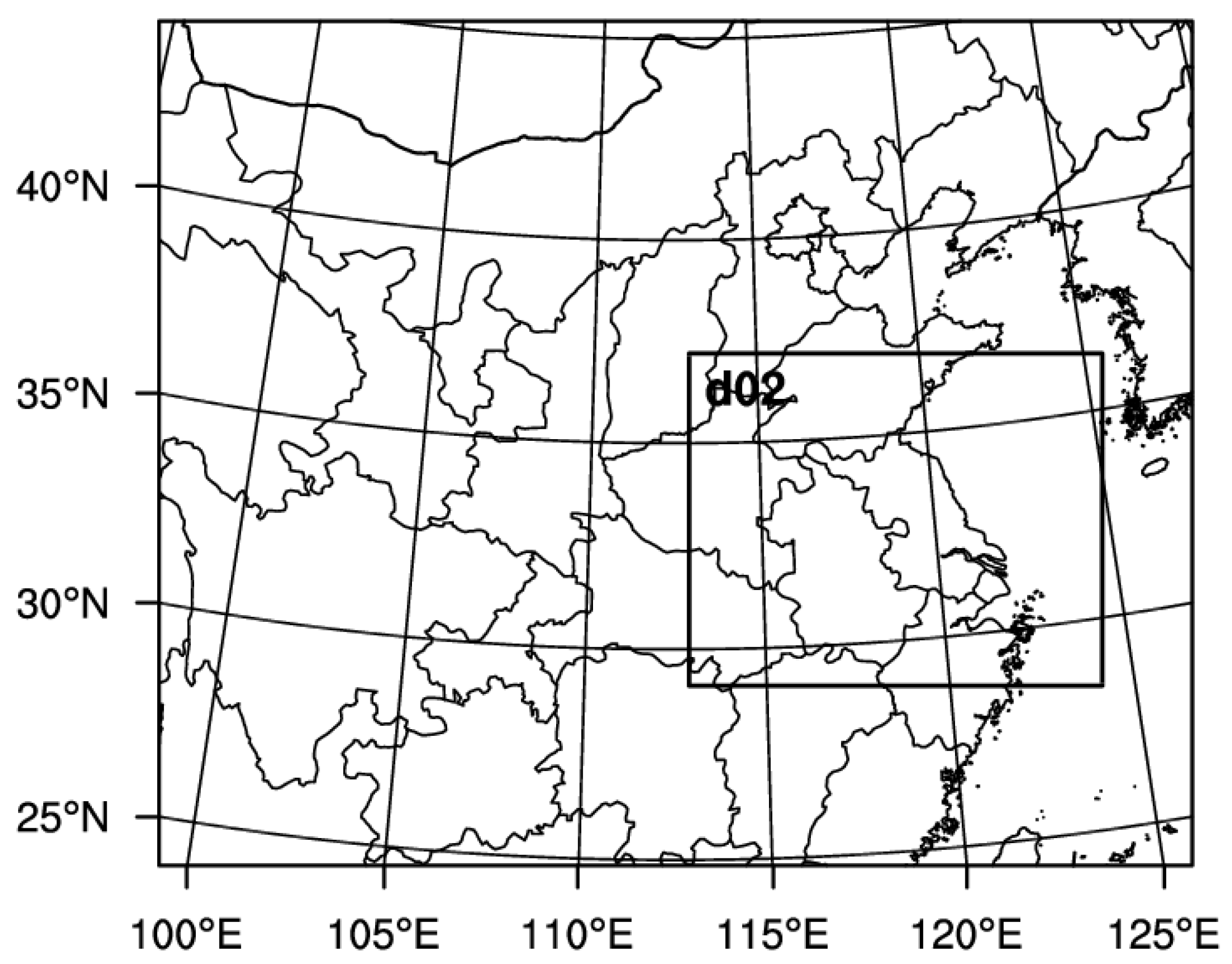
2.1. Model Configurations

The Advanced Research core of the Weather Research and Forecasting (WRF) model version 4.0 is used and two one-way nested domains are employed. The outer domain covered the main areas of China with 116 ×   96 horizontal grid points at 24-km grid spacing, while the inner domain covered the regions of the YHRB, including Anhui and Jiangsu provinces and the surrounding areas with 276 ×   222 horizontal grid points at 4-km grid spacing (Figure 1). All domains contained 38 terrain-following hydrostatic-pressure vertical levels topped at 50 hPa.
The ICs and LBCs were extracted from the European Centre for Medium-Range Weather Forecasts (ECMWF) 0.25° × 0.25° global reanalysis data. Based on the assumption of perfect model, this paper regards the control experiment as the true value field to ignore the influence brought by the MO error. Thus, the physical schemes were independently set for the control experiments of the two cases (Table 1). Besides, the hourly CMORPH data with the resolution of 0.1° provided by the China National Information Center is used for the precipitation forecast evaluation (http://data.cma.cn/; accessed on 16 September 2021).

2.2. Ensemble Design

The CAEFs in this study incorporate LBPs generated through the dynamic downscaling method. The method has been widely used in a number of operational EPSs because of its simplicity, low computational cost, and good performance [14]. Referring to this method, the analysis perturbations from the first 20-member ECMWF global ensemble forecast products (0.5°, https://apps.ecmwf.int/datasets/; accessed on 23 March 2022) were added to the U, V, T, and Qv in ICs and LBCs of the outer domain, so as to provide the IC and LBC perturbations for the outer domain. The LBPs of the inner domain is provided by the forecasts of the outer domain.
We mainly focused on the 24-h ensemble forecasts in the inner to elucidate the relationship between the forecast error evolution and precipitation uncertainty in this scenario, because the error growth due to LBPs influences the precipitation forecasts in such a small domain with a 4-km resolution [72]. Notably, the multi-scale characteristics of forecast error evolution arising from merely LBPs is investigated by using a perfect model assumption [73].
Similar to Xu et al. [74], a set of perturbation magnitude sensitivity ensemble forecasts (Table 2) are conducted to further explore the predictability through multiplying the perturbed fields by different constant factors (0.1, 0.5, and 1.5), corresponding to Per0.1, Per0.5, and Per1.5, respectively.

2.3. Forecast Error Metrics

As in Zhang et al. [45,75], the difference total energy (DTE), used to quantify the error growth procedure, was defined as:
DTE x , t = 1 2 Δ u 2 + Δ v 2 + c p T r Δ T 2 ,
where Δ indicates the difference of u, v, and T between each ensemble member and the unperturbed control run, T r is the reference temperature of 287 K, while c p is specific heat capacity in dry air at constant pressure ( c p = 1004 J·Kg−1·K−1). The occurrence and development of severe convective weather are affected by the environmental fields at different height levels and scales while the traditional DTE can solve the forecast error at a single height level alone. Given this situation, Nielsen and Schumacher [76] applied a vertical function to calculate the two–dimensional root mean vertically integrated DTE (RMDTE):
RMDTE i , j , t = 1 n m = 1 n k = 0 l p k + 1 p k p l p 0 × DTE ,
RMDTE t = 1 n x i = 0 n x 1 n y j = 0 n y RMDTE i , j , t ,
where n indicates the number of ensemble members, l stands for the vertical levels, p is the value of pressure, and n x and n y are the numbers of the grid points in the meridional and zonal directions, respectively. To quantify the evolution characteristics of forecast error at different scales, the discrete cosine transform method (DCT) [77] is used to decompose the forecasts into three scales: the small-scale (48 km wavelength), the medium-scale (120 km wavelength > 48 km), and the large-scale (wavelength > 120 km) [78,79].

2.4. Precipitation Uncertainties Metrics

A quantitative method [80,81] was employed to evaluate the forecast error growth associated with spatial precipitation uncertainties. As mentioned in Surcel et al. [81], by applying this methodology to two or more precipitation fields, a decorrelation scale λ 0 can be defined such that all scales smaller than λ 0 are fully decorrelated. For the scale λ λ 0 , there is no predictability of the model state (precipitation forecasts from ensemble members). For the scale λ > λ 0 , the ensemble forecast members are correlated, indicating some predictability in CAEFs. The power ratio of the decorrelation scale was defined in Surcel et al. [81] as follows:
R λ = i = 1 N P X i λ P X T λ ,
where P X i λ is the variance of the precipitation field X i at scale λ , and N indicates the number of ensemble forecast members. The values for R λ vary between 1/N and 1, where the value of 1 represents complete decorrelation between the fields X i at scale λ , while the value of 1/N represents perfect resemblance between the fields at scale λ . The value of λ 0 was determined by finding the largest λ for which R λ 0.9. The threshold of 0.9 was chosen rather than 1 in this study to eliminate some of the noise without introducing any significant bias in determining the decorrelation scale [82].

3. Case Studies

This study selected two representative severe convective cases that occurred in the YHRB under different forcing mechanisms (regarding the strength of synoptic-scale forcing) during the Meiyu period. Two 24-h ensemble forecasts with initial times of 1200 UTC on 29 June 2015 and 0000 UTC on 26 July 2018 (hereafter Case 1 and 2, respectively) are conducted to examine the differences in the characteristics of forecast error growth and precipitation predictability based on LBPs in different forcing scenarios. Figure 2 shows the precipitation distribution of the two cases. Case 1 is a typical Meiyu frontal rainfall, while Case 2 belongs to locally warm-sector precipitation. As discussed in the introduction, the term “synoptic-scale forcing” is commonly used to classify the strong- and weak-forcing regime, which refers to nonlocal reasons for upward motion, such as quasi-equilibrium forcing for ascent or meso- α meteorological features such as fronts [60,83,84,85]. This section will comprehensively investigate the precipitation occurrence process, forcing characteristics, and ensemble forecast results of the selected cases.

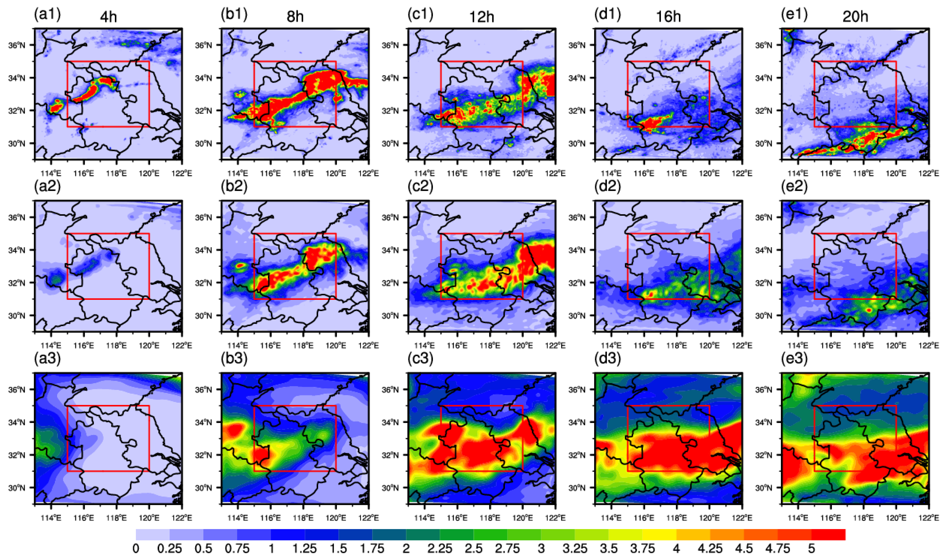
3.1. Case 1: 29 June 2015

The east-west oriented frontal rain belt in Case 1 is mainly composed of the main rain belt in the Huaibei area of Jiangsu and the rain belt in Dabie Mountain of Anhui (Figure 2a). The maximum of 12-h accumulated rainfall exceeded 75 mm during 1600 UTC on 29 June 2015 to 0400 UTC on 30 June 2015. Figure 3 shows the synoptic situation in Case 1. The strong upper-level jet appeared at 200 hPa due to the existence of the South Asian high. There was a deep trough at 500 hPa near Lake Baikal moving southward and deepening, leading to the southward transport of the strong cold air to the YHRB (Figure 3a,b). The existence of the southwest low-level jet and the wind shear line in the analysis area provided abundant water vapor and favorable dynamic uplift conditions, which were both responsible for the rainfall process.
In general, the precipitation occurs in the environmental fields with strong forcing characteristics, where the presence of synoptic systems such as Meiyu front, trough, jet, and the wind shear line provide favorable thermodynamic conditions for precipitation occurrence and development, in line with the previous definitions of the strong-forcing case (SF case) [83,84,85].

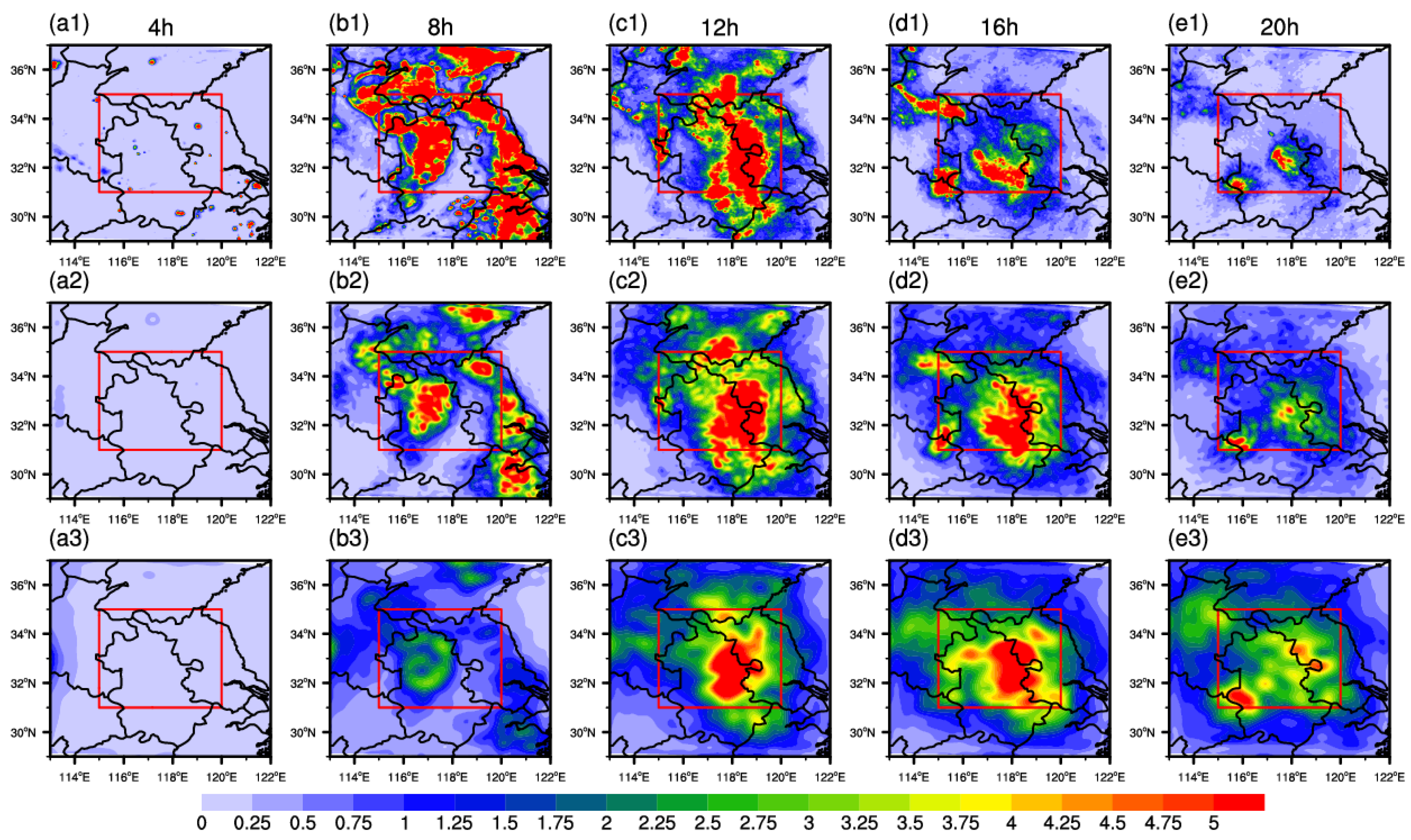
3.2. Case 2: 26 July 2018

The spatial distribution of 12-h precipitation during 0400 UTC on 26 July 2018 to 1600 UTC on 26 July 2018 in Case 2 is shown in Figure 2b. The “popcorn” feature of the precipitation distribution appeared in Anhui and Jiangsu. Figure 4 shows the circulation field in Case 2. In the precipitation region, the upper level was a warm center along with the eastward withdrawal of the 500 hPa subtropical high (Figure 4a blue, black, and green solid line). The southwesterly wind at the middle and low levels provided plenty of water vapor and instability energy to the precipitation process, and there was a convergence area of wind speed at the entrance of the analysis region (Figure 4b,c). Compared with Case 1, this case was mainly driven by the local thermal forcing, which lacked the synoptic forcing systems.
Figure 5 presents the convective available potential energy (CAPE) in the two cases. The CAPE calculated from the control experiments in Case 1 was lower than that of Case 2. Furthermore, a certain vertical upward movement generated by the small-scale convergence at the low levels in the moist unstable environment triggered the release of unstable energy and the occurrence of convection, thus the CAPE value of Case 2 was higher during the first 8-h forecast (daytime), which was consistent with the characteristics of the typical weak-forcing case (WF case) [60].

3.3. Assessment of the Ensemble Forecast

Figure 6 shows the spatial distribution of 12-h accumulated precipitation for ensemble spread and ensemble mean in two cases. The LBP ensemble members in the SF case have a better capture of the location and intensity of the main rain belt occurring in the Huaibei area, but for the Dabie Mountain rain belt, the rainfall is underestimated and the precipitation spread is relatively high (Figure 6a,c). In contrast, in the WF case, there is a good correspondence between precipitation ensemble spread and ensemble mean (Figure 6b,d). The result shows that the impacts of LBPs on the precipitation distribution prediction differ under different forcing mechanisms.
The precipitation time series (the first 4 h of spin-up ignored) in the major precipitation area is also an indicator of the great difference among the ensemble members (dispersion). The dispersion difference caused by the LBPs mainly occurs in the later period of the two cases (Figure 7). In the SF case, the precipitation dispersion becomes larger after a 12-h forecast, consistent with the influence characteristics of LBPs in previous studies [36,38]. However, in the WF case, precipitation dispersion gradually increases with the growth of precipitation and reaches the maximum at the precipitation peak, mainly attributable to the impact of moist convection. Overall, the above results indicate a greater influence of LBPs on the SF case than the WF case.
The growth of forecast errors can partly explain the above differences of precipitation dispersion. Due to the weak autonomy of the system itself in the case of synoptic-scale forcing, different members were developed in different directions induced by forecast errors in the SF case. On the contrary, the forecast errors arising from the LBPs do not play a dominant role in the development of the ensemble members in the WF case, but the nonlinearity error from the moist convection grows. That is, the precipitation dispersion results in two types of cases may be completely different even if the forecast errors from the same source are introduced, which preliminarily reveals the case dependence of LBPs on the predictability of convective events.

4. Characteristics of Forecast Error Growth and Its Influencing Factors

The forecast errors arising from the LBPs can affect the precipitation forecast through error growth and then lead to the ensemble member deviation. This section will further discuss the multi-scale evolution characteristics of forecast errors and its influencing factors.

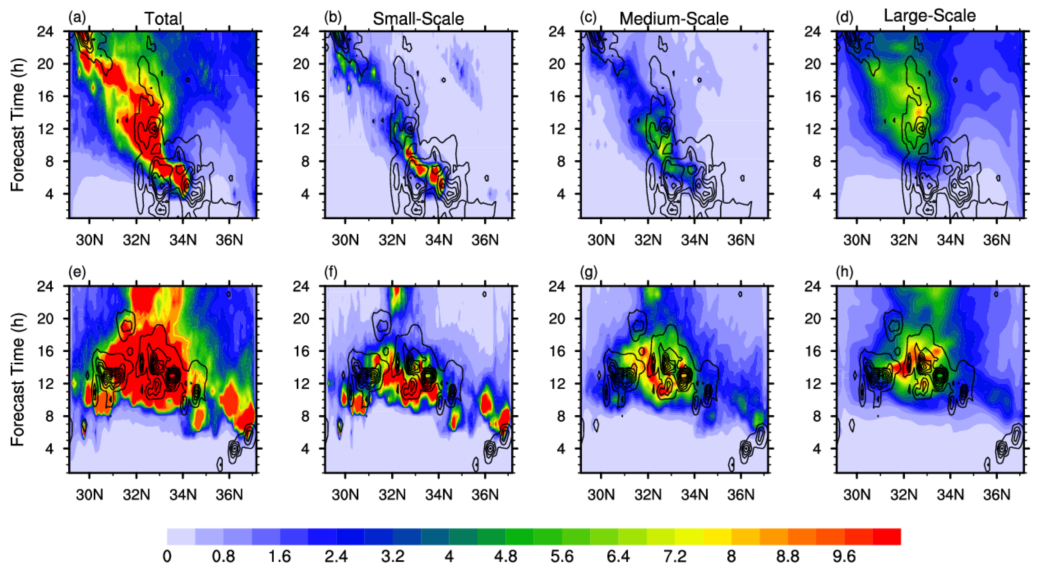
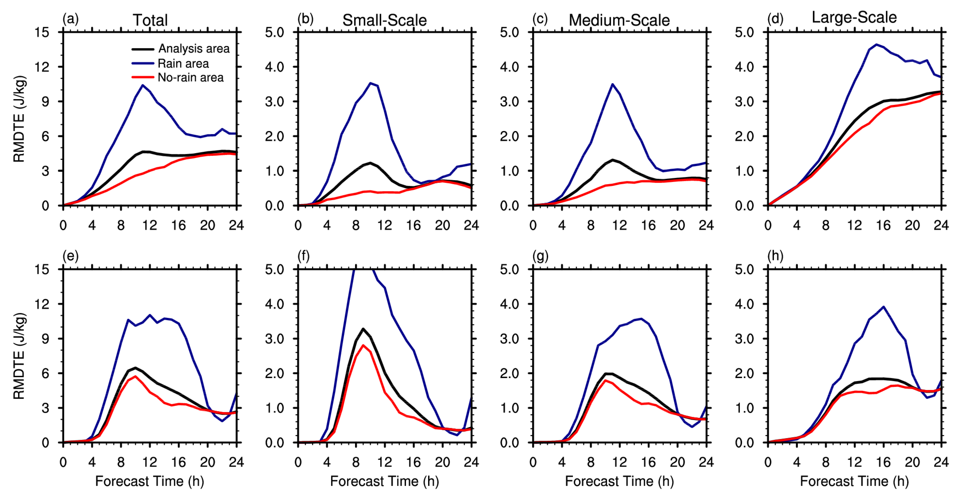
4.1. Spatio-Tempora Evolution Characteristics of Forecast Errors

Figure 8 shows the RMDTE time series and its decomposition at different scales (green line: small-scale, blue line: medium-scale, red line: large-scale) in two cases. In the SF case, the total RMDTE exhibits a steady trend after the rapid increase while a diurnal variation characteristic (a complete wave crest within a 24-h forecast) appears in the WF case (Figure 8a,b).
The spatial propagation of forecast errors varies greatly between the two cases as well (Figure 9 and Figure 10). The total RMDTE in the SF case presents certain eastward zonal and southward meridional propagation, which is more consistent with the moving path of the Meiyu-front system. In contrast, the total RMDTE in the WF case is restricted to a limited area and there is no clear propagation trend, which further reveals the leading role of local moist convection in the error growth of the WF case [75].
For the forecast error components at different scales, the RMDTEs at all scales start from 0 (Figure 8a,b) because no IC perturbations are introduced in the analysis area. In the SF case, the RMDTEs at different scales almost increase synchronously in the early forecast period, while the evolution of multi-scale RMDTEs in the WF case clearly show the upscale transfer processes. This result reflects the different influence mechanisms that determine the growth of forecast errors in the two cases.
For the SF case, the evolution of large-scale errors is affected by LBPs, leading to the large-scale RMDTE increasing after a 12-h forecast (Figure 8a) and almost covering the entire analysis region (Figure 9d and Figure 10d). However, the medium- and small-scale RMDTEs gradually decrease after 12 h and mainly distribute in the precipitation area (Figure 9b,c and Figure 10b,c). This may be due to the slower downscaling propagation speed of large-scale errors in the SF case. Figure 11 shows the distribution of RMDTE at different valid times across different spatial scales in the SF case. Besides, the changes in the synoptic-scale system have more impacts on the spatial propagation characteristics of the large-scale RMDTE. The initial small-scale RMDTE appears in the precipitation region and gradually dissipates as the convection weakens, while the initial large-scale RMDTE is mainly distributed at the boundary and then propagates to the convection region with a broader area. It is speculated this is due to the large-scale errors imposed from the western boundary which directly promotes the forecast errors through the westerly flow at the large scale. The result indicates that the spatial propagation characteristics of the large-scale errors in the SF case is more reflected by the changes in the synoptic-scale system. Therefore, introducing LBPs that contain large-scale errors is preferred for the cases where the synoptic-scale forcing prevails.
By contrast, for the WF case, the small-scale RMDTE has a nonlinearly sharp rise and exceeds the large-scale RMDTE after 4 h (Figure 9b). This is due to the growth of small-scale errors that is mainly caused by the strong nonlinear effect of the moist convection in the absence of synoptic-scale forcing. Besides, the evolution of multi-scale RMDTEs present stepwise saturation characteristics in the WF case: the small-scale RMDTE reaches saturation first, followed by the medium-scale RMDTE and the large-scale RMDTE (Figure 9b). This result implies that the errors arising from the lateral boundary in the WF case essentially follow the three-stage error growth conceptual model [43,44]. Inconsistent with the SF case, the forecast errors at small scale in the WF case grow consistently under the influence of moist convection and impact the large-scale errors via upscale transfer, consistent with the stepwise three-stage error growth model. Another indicator of the error upscale growth process is the spatial distribution of errors at different scales (Figure 12). The smaller scale errors dissipate during 8-16 h, while the area of larger scale errors gradually enlarges. Since the large-scale errors mostly develop from the upscale process of small-scale errors in the WF case, LBPs contribute a little to the dispersion.
It is vital to notice that the difference in scale-dependent evolution trends of forecast errors arising from LBPs between two cases can be linked to the meteorological nature (the strength of synoptic-scale forcing), which reveals the dependence of LBPs on the forcing types, and also reveals the complexity of predicting convective events in the YHRB.

4.2. Relationship between Error Growth and Precipitation Uncertainty

The quantitatively and scale-dependent relationship between forecast error growth and associated precipitation forecasts is investigated in this subsection. We mainly focus on the corresponding characteristics of precipitation uncertainties because the evolution of forecast error energy is closely linked to the precipitation forcing mechanisms (the strength of synoptic-scale forcing) and varies between the two cases.
Figure 13 shows the spectral distribution of power ratio (R) at different forecast lead times for both cases. The two gray lines along the y-axis divide three bands: meso-γ scales (2–20 km), meso-β scales (20–200 km), and meso-α scales (200–2000 km) [86]. The red reference lines indicate the threshold of 0.9, and the precipitation smaller than the corresponding scale will lose all predictability when the R-value exceeds this threshold [80]. In general, the R-value synchronously increases with the forecast hour while varies oppositely with the scale growth. This indicates that the precipitation predictability is lost more rapidly at longer forecast times and smaller scales.
At the early stage of the forecast, the small-scale errors first appeared in the precipitation area and gradually increased (Figure 8, Figure 11 and Figure 12), corresponding to the rapid increase in R-value at a scale smaller than 20 km in two cases. This shows that the initial uncertainty of the precipitation forecast is only reflected in the small-scale part. After the saturation of small-scale errors, the meso-γ scale R almost reaches the threshold line of 0.9, implying that the meso-γ scale storms such as supercells or other systems have completely lost predictability. Meanwhile, the meso-β scale R begins to increase and affects the predictability of the meso-β scale precipitation systems, corresponding to the variation in the pattern and distribution (location) of precipitation.
By comparing the variation of R-value between two cases during the first 10 h, the impact of forecast errors arising from LBPs on precipitation in the WF case is slower than that in the SF case. However, the power ratios of the two cases were different in the later time. In the SF case, the R values in all scales were within the range of the predictable threshold after 12 h. The spatial uncertainty of precipitation in the late forecast of the SF case mainly depends on large-scale errors, which explains the precipitation dispersion caused by LBPs increases after 12 h. While in the WF case, the meso-β scale R-value gradually increases after 10 h, corresponding to the impact of the forecast errors on the precipitation forecast transferring from the smaller scale convection center to the larger scale stratiform rain band along with the upscale growth of errors, and finally affects the whole precipitation field.
Overall, the above results show a close relationship between the source and scale of forecast errors and the precipitation spatial uncertainty, and the relationship differs under different forcing backgrounds. Under different forcing backgrounds, the introduction of LBPs from the same source cause different evolution characteristics of forecast errors, which further leads to great differences in precipitation uncertainty. The precipitation predictability of the SF case driven by LBPs is substantially greater than that in the WF case, corresponding to the differences in the meso-β scale precipitation.

4.3. Influence of Moist Effect on the Error Growth

The previous subsection reveals that the growth of forecast errors caused by LBPs leads to large differences in the precipitation uncertainty between the two cases. Conversely, the moist process can also react to the error growth to a certain extent [43,45,46,87]. To be intuitive, the analysis domain is divided into dry and wet subdomains regarding the hourly precipitation threshold of 0.5 mm·h−1. The evolutions of forecast errors in the rain and no-rain areas are further compared between the two selected cases.
The evolution of domain-averaged RMDTE in the analysis area, rain area, and no-rain area is shown in Figure 14. In the rain area, the RMDTEs increase faster in both cases (blue line in Figure 14), while the RMDTE evolution of two cases differs in the no-rain area (red line in Figure 14). For the SF case, the RMDTE in the no-rain area becomes smaller and the fluctuations associated with moist convection diminish. Conversely, the evolutions of RMDTEs in three areas are almost identical in the WF case, similar to the evolution of precipitation. The continuous influence of moist convection on the propagation of forecast errors from the convection area to the no-rain area is likely the cause, which further demonstrates the importance of the moist convection in the error growth of the WF case. Besides, the promoting effect of moist convection is more evident at the small-scale errors in both cases, indicating that the forecast errors caused by LBPs still rapidly develops downscale through the moist convection even though no IC perturbations are introduced.
As a whole, the moist process accelerates the forecast error growth in two cases, especially for the small-scale errors, and it also promotes the downscaling transmission of forecast errors arising from LBPs. In addition, the differences in the no-rain area error evolution mainly determined by the convection characteristics, indicating that the impact of synoptic-forcing types on the forecast error growth is huge.

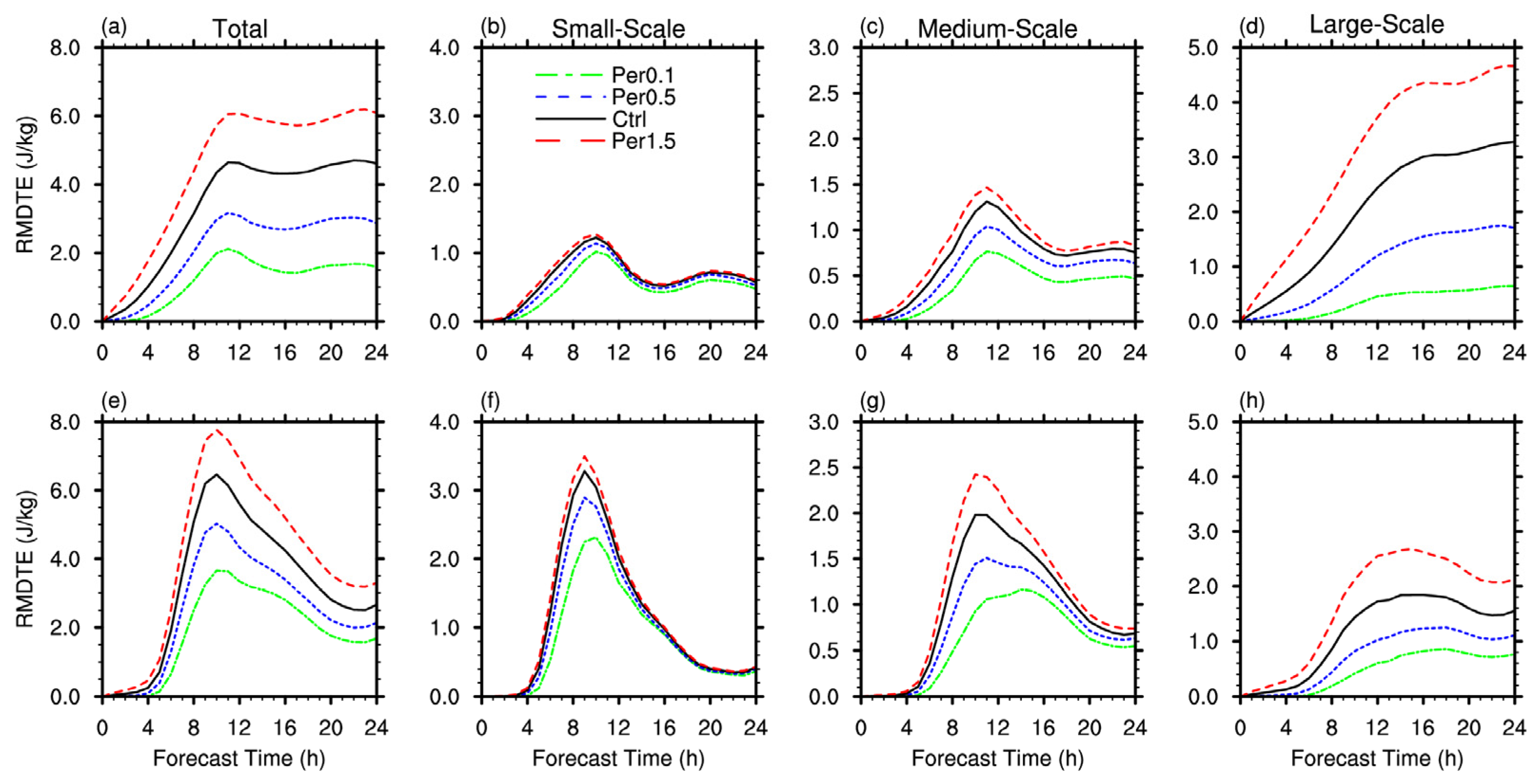
5. Sensitivity Test of Lateral Boundary Perturbations Magnitude

The large-scale errors can propagate from the low-resolution outer domain to the inner region through one-way LBCs, which has an impact on the forecast error growth in CAEF. This section further compares the sensitivity to the magnitude of the LBPs in two cases and discusses the convective-scale predictability of the cases under different forcing backgrounds through the deviation of each sensitivity test.
Figure 15 shows the temporal evolution of domain-averaged RMDTEs for ensemble forecasts with different LBPs magnitudes. The differences in the RMDTE evolution between two cases (Figure 15a,e) can not only illustrate the sensitivity to the LBPs but also further reflect the case-dependent predictability. In the SF case, the total RMDTE evolution with different perturbation magnitudes diverges greatly at the early stage (Figure 15a). Conversely, the deviation among sensitivity tests is not evident in the first 4 h, and presents a trend of convergence after a 10-h forecast (Figure 15e). This suggests that the SF case is more sensitive to the LBPs magnitude than the WF case. At the purely theoretical limit of practical predictability, the beginning and ending RMDTEs are scaled by the proportion to the perturbation scaling, that is, the reduction in the propagation of the ensemble perturbation should lead to a modest reduction in the ensemble dispersion over time [76]. Based on this, the evolution characteristics of RMDTEs in each ensemble for the SF case indicates that the strong-forcing process is more influenced by practical predictability. However, the point of bifurcation in the WF case shows the forecast errors in the late stage cannot be further reduced by adjusting the magnitude of LBPs, which reveals that the weak-forcing process is limited by intrinsic predictability.
From the perspective of each scale, the difference of the RMDTEs is the smallest at the small-scale in two cases, followed by that at the medium-scale and large-scale. In the SF case, the evolution of large-scale RMDTE among four tests is similar to the total RMDTE (Figure 15a,d), while the small-scale RMDTE of each test shows almost no difference (Figure 15b). It indicates that the sensitivity to the LBPs magnitude is mainly reflected in the large-scale rather than small-scale part, which is related to the slow downscaling speed of the large-scale errors. For the WF case, the convergence characteristic appears after a 12-h forecast and more evidently at small- and medium-scale (Figure 15f,g), suggesting that a larger intrinsic predictability limit exists in small- and medium-scale precipitation under the weak-forcing background. Therefore, regarding predictability, introducing large-scale LBPs has little effect on improving the predictability of the WF case, and it is necessary to consider introducing perturbations that can lead to the rapid growth of small- and medium-scale errors.

6. Conclusions

The present study focuses on the forecast error growth arising from LBPs, which is less concerned by previous studies compared with IC and MO perturbations. The multi-scale evolution characteristics of the forecast errors arising from the LBPs in severe convections under different forcing mechanisms over YHRB of East China are preliminarily analyzed to reveal the dependence on the forcing types of severe convection and the adaptability of LBPs in different scenarios. The main conclusions are as follows.
Firstly, the forcing types greatly affect the evolution of forecast errors arising from LBPs. Under strong-forcing condition, the change of the synoptic-scale system determines the growth of forecast errors, and the downscaling propagation speed of the large-scale errors is slow, leading to the large-scale errors being dominant. In contrast, the large-scale errors are mostly developed by upscaling of small-scale errors and are less affected by LBPs in a weak-forcing case in which the growth of forecast errors satisfies the three-order growth characteristics proposed by predecessors [43,44].
Secondly, the difference in the evolution of forecast errors is a cause the difference in precipitation dispersion. The LBPs contribute greatly to the precipitation dispersion in the late forecast period of the SF case, while they cannot produce enough precipitation dispersion in the WF case. Thus, from the perspective of precipitation dispersion, merely LBPs cannot satisfy the requirements of ensemble forecast in the WF case.
In addition, moist convection promotes the growth of forecast errors in two cases, and has a greater influence on the small-scale errors in the WF case than the SF case, corresponding to the rapid downscaling of LBPs through the moist convection region. Besides, the effect of the forcing types on the forecast error growth differs, which is a cause of the difference of the error evolution in the no-rain area between the two cases. The error growth of the SF case in the no-rain area loses the fluctuation related to convection.
Finally, the SF case is more sensitive to the magnitude of the LBPs than the WF case, and the strong-forcing process is more affected by the practical predictability. However, LBPs have little impact on the late time of the weak-forcing process, which is controlled by the intrinsic predictability.
Overall, large-scale LBPs promote error growth and are conducive to large precipitation dispersion under strong synoptic forcing. In contrast, LBPs cannot provide enough ensemble dispersion for the weak-forcing case, thus perturbations from other sources should be considered, which will be further studied in the future work.

Author Contributions

Conceptualization, L.Z., X.Z. and J.M.; methodology, L.Z. and X.Z.; formal analysis, L.Z. and X.Z.; investigation, L.Z. and X.Z.; data curation, L.Z. and X.Z.; writing—original draft preparation, L.Z.; writing—review and editing, L.Z., S.W. and X.Q.; visualization, L.Z.; supervision, J.M.; funding acquisition, J.M. and X.Z. All authors have read and agreed to the published version of the manuscript.

Funding

This research was funded by the National Key Research and Development Program of China (2017YFC1502103), the National Natural Science Foundation of China (42105008) and National Key R&D Program of China (2021YFC3000902).

Institutional Review Board Statement

Not Applicable.

Informed Consent Statement

Not Applicable.

Data Availability Statement

Not Applicable.

Conflicts of Interest

The authors declare no conflict of interest.

References

  1. Ding, Y. Study on the Lasting Heavy Rainfalls over the Yangtze-Huaihe River Basin in 1991; Chinese Meteorological Press Beijing: Beijing, China, 1993. [Google Scholar]
  2. Sun, J.; Zhang, F. Impacts of Mountain-Plains Solenoid on Diurnal Variations of Rainfalls along the Mei-Yu Front over the East over the East China Plains. Mon. Weather Rev. 2012, 140, 379–397. [Google Scholar] [CrossRef] [Green Version]
  3. Luo, Y.; Qian, W.; Zhang, R. Gridded hourly precipitation analysis from high-density rain gauge network over the Yangtze-Huai rivers basin during the 2007 Mei-Yu season and comparison with CMORPH. J. Hydrometeorol. 2013, 14, 1243–1258. [Google Scholar] [CrossRef] [Green Version]
  4. Luo, Y.; Gong, Y.; Zhang, D.-L. Initiation and Organizational Modes of an Extreme-Rain-Producing Mesoscale Convective System along a Mei-Yu Front in East China. Mon. Weather Rev. 2014, 142, 203–221. [Google Scholar] [CrossRef] [Green Version]
  5. Luo, Y.; Chen, Y. Investigation of the predictability and physical mechanisms of an extreme-rainfallproducing mesoscale convective system along the Meiyu front in East China: An ensemble approach. J. Geophys. Res. D Atmos. 2015, 120, 593–618. [Google Scholar]
  6. Chen, Y.; Chan, Y.; Chen, T.; He, H. Characteristics analysis of warm-sector rainstorms over the middle-lowers reaches of the Yangtze River. Meteorol. Mon. 2016, 42, 724–731. (In Chinese) [Google Scholar]
  7. Min, J.; Fang, L. Storm Ensemble Forecast Based on the BGM Method. Trans. Atmos. Sci. 2017, 40, 1–12. [Google Scholar]
  8. Leith, C.E. Theoretical Skill of Monte Carlo Forecasts. Mon. Weather Rev. 1974, 102, 409–418. [Google Scholar] [CrossRef]
  9. Wilks, D.S. Statistical Methods in the Atmospheric Sciences, 2nd ed.; International Geophysics Series; Academic Press: Cambridge, MA, USA, 2006; Volume 100, p. 648. [Google Scholar]
  10. Bishop, C.H.; Craig, G.C.; Holt, T.R.; Nachamkin, J.; Chen, J.; Mclay, J.C.; Doyle, J.D.; Thompson, W.T. Regional Ensemble Forecasts Using the Ensemble Transform Technique. Mon. Weather Rev. 2009, 137, 288–298. [Google Scholar] [CrossRef]
  11. Romine, G.S.; Schwartz, C.S.; Berner, J.; Fossell, K.R.; Snyder, C.; Anderson, J.L.; Weisman, M.L. Representing forecast error in a convection-permitting ensemble system. Mon. Weather Rev. 2014, 142, 4519–4541. [Google Scholar] [CrossRef] [Green Version]
  12. Wang, Y.; Bellus, M.; Geleyn, J.-F.; Ma, X.L.; Tian, W.H.; Weidle, F. A New Method for Generating Initial Condition Perturbations in a Regional Ensemble Prediction System: Blending. Mon. Weather Rev. 2014, 142, 2043–2059. [Google Scholar] [CrossRef] [Green Version]
  13. Li, J.; Du, J.; Liu, Y. A comparison of initial condition, multi-physics and stochastic physics-based ensembles in predicting Beijing “7.21” excessive storm rain event. Acta Meteorol. Sin. 2015, 73, 50–71. [Google Scholar]
  14. Weidle, F.; Wang, Y.; Smet, G. On the impact of the choice of global ensemble in forcing a regional ensemble System. Weather Forecast. 2016, 31, 515–530. [Google Scholar] [CrossRef]
  15. Zhang, H.B.; Zhi, X.F.; Chen, J.; Wu, Z.P.; Xia, Y.; Zhang, X.R. Achievement of perturbation methods for regional ensemble forecast. Transac. Atmos. Sci. 2017, 40, 145–157. [Google Scholar]
  16. Buizza, R.; Houtekamer, P.L.; Pellerin, G.; Toth, Z.; Zhu, Y.; Wei, M. A Comparison of the ECMWF, MSC, and NCEP Global Ensemble Prediction Systems. Mon. Weather Rev. 2015, 133, 347–357. [Google Scholar] [CrossRef]
  17. Xue, M.; Thomas, K.W.; Wang, Y.; Brewster, K.; Kuo, Y.H. CAPS real-time storm-scale ensemble and high-resolution forecasts as part of the NOAA Hazardous Weather Testbed 2007 Spring Experiment. In Proceedings of the 22th Conference on Weather Analysis and Forecasting and 18th Conference on Numerical Weather Prediction, Salt Lake City, UT, USA, 25–29 June 2007. [Google Scholar]
  18. Kain, J.S.; Weiss, J.; Bright, R.; Baldwin, E.; Levit, J.; Carbin, W.; Schwartz, S.; Weisman, L.; Droegemeier, K.; Weber, B. Some practical considerations regarding horizontal resolution in the first generation of operational convection-allowing NWP. Weather Forecast. 2008, 23, 931–952. [Google Scholar] [CrossRef]
  19. Gebhardt, C.; Theis, S.E.; Paulat, M.; Bouallègue, Z.B. Uncertainties in COSMO-DE precipitation forecasts introduced by model perturbations and variation of lateral boundaries. Atmos. Res. 2011, 100, 168–177. [Google Scholar] [CrossRef]
  20. Hohenegger, C.; Lüthi, D.; Schär, C. Predictability mysteries in cloud-resolving models. Mon. Weather Rev. 2007, 134, 2095–2107. [Google Scholar] [CrossRef] [Green Version]
  21. Marsigli, C.; Boccanera, F.; Montani, A.; Paccagnella, T. The COSMO-LEPS mesoscale ensemble system: Validation of the methodology and verification. Nonlinear Process. Geophys. 2005, 12, 27–536. [Google Scholar] [CrossRef] [Green Version]
  22. Frogner, I.L.; Haakenstad, H.; Iversen, T. Limited-area ensemble predictions at the Norwegian Meteorological Institute. Q. J. R. Meteorol. Soc. 2006, 132, 2785–2808. [Google Scholar] [CrossRef]
  23. Bowler, N.E.; Arribas, A.; Mylne, K.R.; Robertson, K.B.; Beare, S.E. The MOGREPS short-range ensemble prediction system. Q. J. R. Meteorol. Soc. 2008, 134, 703–722. [Google Scholar] [CrossRef]
  24. Wang, Y.; Bellus, M.; Wittmann, C.; Steinheimer, M.; Weidle, F.; Kann, A.; Ivatek-Sahdan, S.; Tian, W.H.; Ma, X.L.; Tascu, S.; et al. The Central European limited-area ensemble forecasting system: ALADIN-LAEF. Q. J. R. Meteorol. Soc. 2011, 137, 483–502. [Google Scholar] [CrossRef]
  25. Zhang, H.B.; Chen, J.; Zhi, X.F.; Wang, Y.N. A comparison of ETKF and downscaling in a regional ensemble prediction system. Atmosphere 2015, 6, 341–360. [Google Scholar] [CrossRef]
  26. Hagelin, S.; Son, J.; Swinbank, R.; McCabe, A.; Roberts, N.; Tennant, W. The Met Office convective-scale ensemble, MOGREPS-UK. Q. J. R. Meteorol. Soc. 2017, 143, 2846–2861. [Google Scholar] [CrossRef]
  27. Schwartz, C.S. Medium-range convection-allowing ensemble forecasts with a variable-resolution global model. Mon. Weather Rev. 2019, 147, 2997–3023. [Google Scholar] [CrossRef]
  28. Johnson, A.; Wang, X. A study of multiscale initial condition perturbation methods for convection-permitting ensemble forecasts. Mon. Weather Rev. 2016, 144, 2579–2604. [Google Scholar] [CrossRef]
  29. Zhang, X.Y.; Min, J.Z.; Wu, T.J. A study of ensemble-sensitivity-based initial condition perturbation methods for convection-permitting ensemble forecasts. Atmos. Res. 2020, 234, 104741. [Google Scholar] [CrossRef]
  30. Wang, S.; Qiao, X.; Min, J.; Zhuang, X. The impact of stochastically perturbed parameterizations on tornadic supercell cases in east China. Mon. Weather Rev. 2019, 147, 199–220. [Google Scholar] [CrossRef]
  31. Feng, Y.; Janjić, T.; Zeng, Y.; Seifert, A.; Min, J. Representing microphysical uncertainty in convective-scale data assimilation using additive noise. J. Adv. Model. Earth Syst. 2021, 13, e2021MS002606. [Google Scholar] [CrossRef]
  32. Saito, K.; Kuroda, K.; Kunii, M.; Kohno, N. Numerical simulation of Myanmar cyclone Nargis and the associated storm surge Part II: Ensemble prediction. J. Meteorol. Soc. Jpn. 2010, 88, 547–570. [Google Scholar] [CrossRef] [Green Version]
  33. Saito, K.; Seko, H.; Kunii, M.; Miyoshi, T. Effect of lateral boundary perturbations on the breeding method and the local ensemble transform Kalman filter for mesoscale ensemble prediction. Tellus A 2012, 64, 11594. [Google Scholar] [CrossRef] [Green Version]
  34. Marsigli, C.; Montani, A.; Paccagnella, T. Provision of boundary conditions for a convection-permitting ensemble: Comparison of two different approaches. Nonlinear Process. Geophys. 2014, 21, 393–403. [Google Scholar] [CrossRef] [Green Version]
  35. Nutter, P.; Stensrud, D.; Xue, M. Effects of Coarsely Resolved and Temporally Interpolated Lateral Boundary Conditions on the Dispersion of Limited-Area Ensemble Forecasts. Mon. Weather Rev. 2004, 132, 2358–2377. [Google Scholar] [CrossRef]
  36. Nutter, P.; Xue, M.; Stensrud, D. Application of lateral boundary condition perturbations to help restore dispersion in limited-area ensemble forecasts. Mon. Weather Rev. 2004, 132, 2378–2390. [Google Scholar] [CrossRef]
  37. Hohenegger, C.; Walser, A.; Langhans, W.; Schär, C. Cloud-resolving ensemble simulations of the August 2005 Alpine flood. Q. J. R. Meteorol. Soc. 2008, 134, 889–904. [Google Scholar] [CrossRef]
  38. Vié, B.; Nuissier, O.; Ducrocq, V. Cloud-Resolving Ensemble Simulations of Mediterranean Heavy Precipitating Events: Uncertainty on Initial Conditions and Lateral Boundary Conditions. Mon. Weather Rev. 2011, 139, 403–423. [Google Scholar] [CrossRef]
  39. Peralta, C.; Ben Bouallègue, Z.; Theis, S.E.; Gebhardt, C.; Buchhold, M. Accounting for initial condition uncertainties in COSMO-DE-EPS. J. Geophys. Res. Atmos. 2012, 117. [Google Scholar] [CrossRef]
  40. Kühnlein, C.; Keil, C.; Craig, G.C.; Gebhardt, C. The impact of downscaled initial condition perturbations on convective-scale ensemble forecasts of precipitation. Q. J. R. Meteorol. Soc. 2014, 140, 1552–1562. [Google Scholar] [CrossRef]
  41. Zhang, X. Multiscale characteristics of different-source perturbations and their interactions for convection-permitting ensemble forecasting during SCMREX. Mon. Weather Rev. 2019, 147, 291–310. [Google Scholar] [CrossRef]
  42. Johnson, A.; Wang, X.; Xue, M.; Kong, F.; Zhao, G.; Wang, Y.; Thomas, K.W.; Brewster, K.A.; Gao, J. Multiscale Characteristics and Evolution of Perturbations for Warm Season Convection-Allowing Precipitation Forecasts: Dependence on Background Flow and Method of Perturbation. Mon. Weather Rev. 2014, 142, 1053–1073. [Google Scholar] [CrossRef]
  43. Zhang, F.Q.; Bei, N.F.; Rotunno, R.; Snyder, C.; Epifanio, C.C. Mesoscale Predictability of Moist Baroclinic Waves: Convection-Permitting Experiments and Multistage Error Growth Dynamics. J. Atmos. Sci. 2007, 64, 3579–3594. [Google Scholar] [CrossRef]
  44. Selz, T.; Craig, G.C. Upscale Error Growth in a High-Resolution Simulation of a Summertime Weather Event over Europe. Mon. Weather Rev. 2015, 143, 813–827. [Google Scholar] [CrossRef]
  45. Zhang, F.Q.; Snyder, C.; Rotunno, R. Effects of Moist Convection on Mesoscale Predictability. J. Atmos. Sci. 2003, 60, 1173–1185. [Google Scholar] [CrossRef]
  46. Hohenegger, C.; Schär, C. Predictability and error growth dynamics in cloud-resolving models. J. Atmos. Sci. 2007, 64, 4467–4478. [Google Scholar] [CrossRef]
  47. Bei, N.F.; Zhang, F.Q. Impacts of initial condition errors on mesoscale predictability of heavy precipitation along the Mei-Yu front of China. Q. J. R. Meteorol. Soc. 2007, 133, 83–99. [Google Scholar] [CrossRef]
  48. Melhauser, C.; Zhang, F.Q. Practical and Intrinsic Predictability of Severe and Convective Weather at the Mesoscales. J. Atmos. Sci. 2012, 69, 3350–3371. [Google Scholar] [CrossRef]
  49. Sun, Y.Q.; Zhang, F.Q. Intrinsic versus practical limits of atmospheric predictability and the significance of the butterfly effect. J. Atmos. Sci. 2016, 73, 1419–1438. [Google Scholar] [CrossRef] [Green Version]
  50. Bierdel, L.; Selz, T.; Craig, G.C. Theoretical aspects of upscale error growth through the mesoscales: An analytical model. Q. J. R. Meteorol. Soc. 2017, 143, 3048–3059. [Google Scholar] [CrossRef]
  51. Argence, S.; Lambert, D.; Richard, E.; Chaboureau, J.P.; Söhne, N. Impact of initial condition uncertainties on the predictability of heavy rainfall in the Mediterranean: A case study. Q. J. R. Meteorol. Soc. 2008, 134, 1775–1788. [Google Scholar] [CrossRef]
  52. Durran, D.R.; Gingrich, M. Atmospheric predictability: Why butterflies are not of practical importance. J. Atmos. Sci. 2014, 71, 2476–2488. [Google Scholar] [CrossRef]
  53. Durran, D.R.; Weyn, J.A. Thunderstorms do not get butterflies. Bull. Am. Meteorol. Soc. 2016, 97, 237–243. [Google Scholar] [CrossRef]
  54. Weyn, J.A.; Durran, D.R. The dependence of the predictability of mesoscale convective systems on the horizontal scale and amplitude of initial errors in idealized simulations. J. Atmos. Sci. 2017, 74, 2191–2210. [Google Scholar] [CrossRef]
  55. Selz, T.; Bierdel, L.; Craig, G.C. Estimation of the variability of mesoscale energy spectra with three years of COSMO-DE analyses. J. Atmos. Sci. 2019, 76, 627–637. [Google Scholar] [CrossRef]
  56. Done, J.M.; Craig, G.C.; Gray, S.L.; Clark, P.A.; Gray, M.E.B. Mesoscale simulations of organized convection: Importance of convective equilibrium. Q. J. R. Meteorol. Soc. 2006, 132, 737–756. [Google Scholar] [CrossRef] [Green Version]
  57. Keil, C.; Craig, G.C. Regime-dependent forecast uncertainty of convective precipitation. Meteorol. Z. 2011, 20, 145–151. [Google Scholar] [CrossRef]
  58. Flack, D.L.A.; Plant, R.S.; Gray, S.L.; Lean, H.W.; Keil, C.; Craig, G.C. Characterisation of convective regimes over the British Isles. Q. J. R. Meteorol. Soc. 2016, 142, 1541–1553. [Google Scholar] [CrossRef]
  59. Done, J.M.; Craig, G.C.; Gray, S.L.; Clark, P.A. Case-to-case variability of predictability of deep convection in a mesoscale model. Q. J. R. Meteorol. Soc. 2012, 138, 638–648. [Google Scholar] [CrossRef]
  60. Surcel, M.; Zawadzki, I.; Yau, M.K. The case-to-case variability of the predictability of precipitation by a storm-scale ensemble forecasting system. Mon. Weather Rev. 2016, 144, 193–212. [Google Scholar] [CrossRef]
  61. Keil, C.; Baur, F.; Bachmann, K.; Rasp, S.; Schneider, L.; Barthlott, C. Relative contribution of soil moisture, boundary-layer and microphysical perturbations on convective predictability in different weather regimes. Q. J. R. Meteorol. Soc. 2019, 145, 3102–3115. [Google Scholar] [CrossRef]
  62. Bachmann, K.; Keil, C.; Craig, G.C.; Weissmann, M.; Welzbacher, C.A. Predictability of deep convection in idealized and operational forecasts: Effects of radar data assimilation, orography, and synoptic weather regime. Mon. Weather Rev. 2020, 148, 63–81. [Google Scholar] [CrossRef]
  63. Flack, D.L.A.; Gray, S.L.; Plant, R.S.; Lean, H.W.; Craig, G.C. Convective-Scale Perturbation Growth across the Spectrum of Convective Regimes. Mon. Weather Rev. 2018, 146, 387–405. [Google Scholar] [CrossRef]
  64. Weyn, J.A.; Durran, D.R. The scale dependence of initial-condition sensitivities in simulations of convective systems over the southeastern United States. Q. J. R. Meteorol. Soc. 2019, 145, 57–74. [Google Scholar] [CrossRef] [Green Version]
  65. Zhuang, X.R.; Min, J.Z.; Zhang, L.; Wang, S.Z.; Wu, N.G.; Zhu, H.N. Insights into convective-scale predictability in east China: Error growth dynamics and associated impact on precipitation of warm-season convective events. Adv. Atmos. Sci. 2020, 37, 893–911. [Google Scholar] [CrossRef]
  66. Zhang, X.B. Case dependence of multiscale interactions between multisource perturbations for convection-permitting ensemble forecasting during SCMREX. Mon. Weather Rev. 2021, 149, 1853–1871. [Google Scholar] [CrossRef]
  67. Chen, X.; Yuan, H.L.; Xue, M. Spatial spread-skill relationship in terms of agreement scales for precipitation forecasts in a convection-allowing ensemble. Q. J. R. Meteorol. Soc. 2018, 144, 85–98. [Google Scholar] [CrossRef]
  68. Zhao, S.X.; Zhang, L.S.; Sun, J.H. Study of heavy rainfall and related mesoscale systems causing severe flood in Huaihe River basin during the summer of 2007. Clim. Environ. Res. 2007, 12, 713–727. [Google Scholar]
  69. Zhang, M.; Zhang, D.-L. Subkilometer simulation of a torrential-rain-producing mesoscale convective system in East China. Part I: Model verification and convective organization. Mon. Weather Rev. 2012, 140, 184–201. [Google Scholar] [CrossRef]
  70. Fu, S.; Yu, F.; Wang, D.; Xia, R. A comparison of two kinds of eastward-moving mesoscale vortices during the Mei-Yu period of 2010. Sci. China Earth Sci. 2013, 56, 282–300. [Google Scholar] [CrossRef]
  71. Zhang, L.; Min, J.Z.; Zhuang, X.R. Schumacher, R.S. General features of extreme rainfall events produced by MCSs over East China during 2016–17. Mon. Weather Rev. 2019, 147, 2693–2714. [Google Scholar] [CrossRef]
  72. Zhuang, X.R.; Wu, N.G.; Min, J.Z.; Xu, Y. Understanding the predictability within convection-allowing ensemble forecasts in east China: Meteorological sensitivity, forecast error growth and associated precipitation uncertainties across spatial scales. Atmosphere 2020, 11, 234. [Google Scholar] [CrossRef]
  73. Flora, M.L.; Potvin, C.K.; Wicker, L.J. Practical Predictability of Supercells: Exploring Ensemble Forecast Sensitivity to Initial Condition Spread. Mon. Weather Rev. 2018, 146, 2361–2379. [Google Scholar] [CrossRef]
  74. Xu, Y.; Min, J.Z.; Zhuang, X.R. Predictability Study of Warm-sector Convective Event over the Middle-lower Reaches of the Yangtze River: Based on Convection-allowing Ensemble Simulation. Plateau Meteorol. 2022, 41, 684–697. [Google Scholar]
  75. Zhang, F.; Odins, A.M.; Nielsen-Gammon, J.W. Mesoscale predictability of an extreme warm-season precipitation event. Weather Forecast. 2006, 21, 149–166. [Google Scholar] [CrossRef]
  76. Nielsen, E.R.; Schumacher, R.S. Using Convection-Allowing Ensembles to Understand the Predictability of an Extreme Rainfall Event. Mon. Weather Rev. 2016, 144, 3651–3676. [Google Scholar] [CrossRef]
  77. Denis, B.; Côté, J.; Laprise, R. Spectral Decomposition of Two-Dimensional Atmospheric Fields on Limited-Area Domains Using the Discrete Cosine Transform (DCT). Mon. Weather Rev. 2002, 130, 1812–1829. [Google Scholar] [CrossRef]
  78. Zhuang, X.R.; Min, J.Z.; Cai, Y.C.; Feng, J.W. Optimal design of lateral boundary condition perturbation method in storm-scale ensemble forecast: A case study. J. Meteorol. Sci. 2017, 37, 21–29. [Google Scholar]
  79. Zhuang, X.R.; Xue, M.; Min, J.Z.; Kang, Z.; Kong, F. Error growth dynamics within convection-allowing ensemble forecasts over central U.S. Regions for days of active convection. Mon. Weather Rev. 2021, 149, 959–977. [Google Scholar] [CrossRef]
  80. Surcel, M.; Zawadzki, I.; Yau, M.K. On the Filtering Properties of Ensemble Averaging for Storm-Scale Precipitation Forecasts. Mon. Weather Rev. 2014, 142, 1093–1105. [Google Scholar] [CrossRef]
  81. Surcel, M.; Zawadzki, I.; Yau, M.K. A Study on the Scale Dependence of the Predictability of Precipitation Patterns. J. Atmos. Sci. 2015, 72, 216–235. [Google Scholar] [CrossRef]
  82. Wu, N.G.; Zhuang, X.R.; Min, J.Z.; Meng, Z.Y. Practical and intrinsic predictability of a warm-sector torrential rainfall event in the south China monsoon region. J. Geophys. Res. D Atmos. 2020, 125, e2019JD031313. [Google Scholar] [CrossRef]
  83. Jankov, I.; Gallus, W.A. MCS rainfall forecast accuracy as a function of large-scale forcing. Weather Forecast. 2014, 19, 428–439. [Google Scholar] [CrossRef]
  84. Duda, J.D.; Gallus, W.A. The impact of large-scale forcing on skill of simulated convective initiation and upscale evolution with convection-allowing grid spacings in the WRF. Weather Forecast. 2013, 28, 994–1018. [Google Scholar] [CrossRef] [Green Version]
  85. Zhuang, X.R.; Min, J.Z.; Cai, Y.C.; Zhu, H.N. Convective-scale ensemble prediction experiments under different large-scale forcing with consideration of uncertainties in initial and lateral boundary condition. Acta Meteorol. Sin. 2016, 74, 244–258. [Google Scholar]
  86. Orlanski, I. A rational subdivision of scales for atmospheric processes. Bull. Am. Meteorol. Soc. 1975, 56, 527–530. [Google Scholar]
  87. Leoncini, G.; Plant, R.S.; Gray, S.L.; Clark, P.A. Perturbation growth at the convective scale for CSIP IOP18. Q. J. R. Meteorol. Soc. 2010, 136, 653–670. [Google Scholar] [CrossRef]
Figure 1. Configuration of model domains. The inner domain (d02) is the analysis region.
Atmosphere 14 00176 g001
Figure 2. The spatial distributions of 12-h accumulated precipitation in (a) the SF case and (b) the WF case.
Atmosphere 14 00176 g002
Figure 3. Geopotential heights (black solid line), temperature (red dotted line), and wind field (arrow: wind direction; shadow: full wind speed) at 0000 UTC on 30 June 2015 at the level of (a) 200 hPa; (b) 500 hPa; (c) 700 hPa and (d) 850 hPa. The trough line at 500 hPa (brown line) and the shear line at 850 hPa (black dotted line) are plotted. The black rectangles mark the analysis region shown in Figure 1.
Atmosphere 14 00176 g003
Figure 4. Geopotential heights (black solid line: 1200 UTC 26 July; blue solid line: 0000 UTC 26 July; green solid line: 0000 UTC 27 July), temperature (red dotted line), and wind field (arrow: wind direction; shadow: full wind speed) at 1200 UTC on 26 July 2018 at the level of (a) 500 hPa; (b) 700 hPa; (c) 850 hPa and (d) 925 hPa. The black rectangles mark the analysis region shown in Figure 1.
Atmosphere 14 00176 g004
Figure 5. The time series of the precipitation area-average (>1.0 mm/h) convective available potential energy (CAPE) in two cases (black solid line: SF case, black dotted line: WF case).
Atmosphere 14 00176 g005
Figure 6. Spatial distribution of 12-h accumulated precipitation diagnostics (mm) for the LBP ensemble spread (a,c) and ensemble mean (b,d). Left column: the SF case, right column: the WF case.
Atmosphere 14 00176 g006
Figure 7. The time series of regional average precipitation in the (a) SF case and (b) WF case (red solid line: observation; black dotted line: control experiment; blue solid line: the result of ensemble mean; gray dotted line: ensemble member forecast).
Atmosphere 14 00176 g007
Figure 8. Temporal evolution of the RMDTE in the (a) SF case and (b) WF case at various scales (black line: total RMDTE; red line: large-scale RMDTE; blue line: medium-scale RMDTE; green line: small-scale RMDTE).
Atmosphere 14 00176 g008
Figure 9. Hovmöller diagrams (time-longitude) of the RMDTE (shaded) and the precipitation (contour) at different scales in (ad) the SF case and (eh) the WF case.
Atmosphere 14 00176 g009
Figure 10. Hovmöller diagrams (time-latitude) of the RMDTE (shaded) and the precipitation (contour) at different scales in (ad) the SF case and (eh) the WF case.
Atmosphere 14 00176 g010
Figure 11. Distribution maps of RMDTE in the SF case at (a1e1) the small scale, (a2e2) medium scale, and (a3e3) large scale for (a1a3) 4-h, (b1b3) 8-h, (c1c3) 12-h, (d1d3) 16-h, and (e1e3) 20-h forecasts. The red square marks the major precipitation area.
Atmosphere 14 00176 g011
Figure 12. As in Figure 11, but in the WF case. The red square marks the major precipitation area.
Atmosphere 14 00176 g012
Figure 13. Spectral distribution of the power ratio (R, no unit) at different forecast lead times in the (a) SF case and (b) WF case. The gray lines along the y-axis are 20 and 200 km and the red reference lines indicate the threshold (total loss of predictability) of 0.9.
Atmosphere 14 00176 g013
Figure 14. Time series of the domain-average RMDTE in the rain area (hourly precipitation > 0.5 mm·h−1) and no-rain area (hourly precipitation < 0.5 mm·h−1) at each scale in (ad) the SF case and (eh) the WF case (black line: the whole analysis area; blue line: the rain area; red line: the no-rain area).
Atmosphere 14 00176 g014
Figure 15. Time series of RMDTEs for magnitude sensitivity tests of ensemble forecasts in (ad) the SF case and (eh) the WF case.
Atmosphere 14 00176 g015
Table 1. Model parameter configuration of control experiments.
SchemeCase 1Case 2
Outer DomainInner DomainOuter DomainInner Domain
MicrophysicsFerrierFerrierWDM6WDM6
Boundary layerYSUYSUQNSEQNSE
Cumulus convectionKain-Fritsch/Kain-Fritsch/
Longwave radiationrrtmrrtmrrtmrrtm
Shortwave radiationDudhiaDudhiaDudhiaDudhia
Table 2. Configuration of sensitivity tests for lateral boundary error.
Experiment NameLateral Boundary Perturbation
Ctrl 24 km
Per0.10.1 × 24 km
Per0.50.5 × 24 km
Per1.51.5 × 24 km
Disclaimer/Publisher’s Note: The statements, opinions and data contained in all publications are solely those of the individual author(s) and contributor(s) and not of MDPI and/or the editor(s). MDPI and/or the editor(s) disclaim responsibility for any injury to people or property resulting from any ideas, methods, instructions or products referred to in the content.

