Performance Analysis of a Portable Low-Cost SDR-Based Ionosonde

Abstract

This work presents a software-defined radio ionosonde (ISDR) developed at the Abdus Salam International Centre for Theoretical Physics (Italy) and the Institute of Radio Astronomy (Ukraine) and installed at the Ukrainian Antarctic Station in 2017. For the first time, the results of the long-term data comparison of the ISDR with the conventional ionosonde IPS-42 produced by KEL Aerospace are presented and discussed. The matching of the ionograms obtained during the whole year of 2021, as well as a comparison of the critical frequencies and virtual heights of F, E, and Es layers manually scaled from the ionograms showed that the ISDR has a similar level of performance to IPS-42. At the same time, the ISDR is a more versatile instrument that supports a bistatic operation, provides Doppler measurements and polarization information, and has a significantly lower cost and transmission power. Different configurations of the ISDR are considered. The basic configuration allows for using the ISDR as a conventional vertical ionospheric sounder. An enhanced configuration of the ISDR allows for oblique sounding, as well as polarization information that enables the O- and X-propagation modes of the ionospheric signal to be distinguished. The enhanced passive version of the ISDR was successfully tested onboard the research vessel “Noosfera” on distances up to 1,400 km from the transmitting ISDR.

1. Introduction

Although the ionosonde was invented about one hundred years ago [1,2,3,4], it still remains one of the most versatile and efficient tools for studying the near-Earth plasma. The ionosonde is a high frequency (HF) range radar which, by sweeping the sounding frequency, allows reconstructing of the electron density profile at heights from about a hundred kilometers to the absolute maximum of the plasma frequency, named the critical frequency of the ionosphere. The standard data output of an ionosonde is a graph of the time of the reflection of the signal, usually shown as a virtual height, as a function of the frequency what is called an ionogram. The two most common modulation schemes used in the ionospheric sounding are the chirp modulation, when the frequency of the sinusoidal signal changes linearly with time, and the pulse modulation, when the frequency of the carrier signal changes from one pulse to another. While improving the hardware and measurement techniques, ionosondes have gained the ability to determine not only the signal amplitude and distance to the reflection point, but also the Doppler frequency shift, phase, polarization characteristics, and the angles of arrival of the sounding signals.

The ionosonde, like most other diagnostic tools, has evolved from a relatively simple analog instrument to a fully fledged digital device. Among the most advanced devices, one should point out digisondes, ranging from the model 128PS [5] created in the 1970s to the modern development of DPS4D [6]. A significant advantage of digisondes over other types of ionosondes is the software system called the Automatic Real-Time Ionogram Scaler, with true height calculation (ARTIST) supplied, starting from the model DGS256 [4]. The ARTIST allows the processing of raw ionospheric sounding data (ionograms) in a standard way which is identical for all digisondes, and for obtaining the characteristics of the ionosphere in a digital form in near-real-time. Despite the fact that the scaling of ionograms using the ARTIST is not free from errors and manual processing still remains more reliable [7], specifically, the presence of universal processing software (such as ATRIST) has made it possible to create an effective worldwide network of ionosondes that supplies data to the online portal, the Global Ionosphere Radio Observatory (GIRO) [8].

It should be noted that there is a large number of other models of digital ionosondes whose capabilities are comparable to those of digisondes. They include Canadian Advanced Digital Ionosonde (CADI) [9], VIPIR-Dynasonde [10], AIS-INGV [11], IPS, WIOBSS/WMI [12,13], VISRC2 manufactured by SRC PAS [14], and others. Most of the instruments listed above demonstrate excellent diagnostic capabilities with some advantages or disadvantages over others. Nevertheless, their main downside is the relatively high cost and high radiated power that did not allow for these devices to become widespread instruments for an ionosphere diagnostic as, for example, it happened to other classes of devices used for ionospheric studies, GNSS receivers [15,16,17]. In recent times, however, with the evolution of the software-defined radio (SDR) concept, it has become possible to make ionosondes widely accessible. The developed prototypes of SDR-based ionosondes [18,19,20,21,22,23] combine the smart capabilities of digisondes with the low-cost, low-power, and compact size of SDR-based devices. Nevertheless, for the commissioning of SDR-based ionosonde as the main vertical sounding instrument of an ionospheric observatory, a number of requirements have to be met. It is necessary to ensure the continuity of both: raw ionograms that were previously recorded by a traditional ionosonde, and the basic ionospheric parameters arrays such as foF2, foE, foEs, fmin, h’F, h’E, and h’Es scaled from the ionograms. It is worth noting that the most viable solution for the routine processing of ionograms is their auto-scaling using a generalized software such as the ARTIST [24,25] or AUTOSCALA [26,27].

In this paper, an SDR-based ionosonde (ISDR) developed at the Abdus Salam International Centre for Theoretical Physics (ICTP), Italy, in cooperation with the Institute of Radio Astronomy, National Academy of Sciences of Ukraine (IRA NASU), is described. The results of the long-term performance comparison of the ISDR and the reference instrument, IPS-42, both operating at the Ukrainian Antarctic Station (UAS) “Akademik Vernadsky” (geographic coordinates: 65.25° S 64.25° W; geomagnetic coordinates: 55.8° S 6.3° E), are presented. It should be noted that the geomagnetic coordinates indicate that the ionospheric conditions at the station are mid-latitude despite the subpolar geographic coordinates. IPS-42 produced by KEL Aerospace Pty Ltd (Ashburton, Australia) [28] is the base instrument used for 24 h a day ionospheric diagnostics at the UAS since January 1983. In 2001, the ionosonde was upgraded to record ionograms in digital form [29]. An ISDR was installed at the UAS in 2017 [29,30]. The IPS-42 and the ISDR share the same antenna system and work together in round-the-clock mode until now. In this work, the long-term performance of the two systems is presented for the first time. The differences between the systems are explained and discussed in detail.

The paper also discusses the results of the recent upgrade of the ISDR at the UAS performed by the co-authors from the University of New Brunswick (UNB) in 2022 [31]. The ISDR system was equipped with a GPS disciplined reference clock and a second RX channel. This upgrade allowed establishing a network of bistatic passive ISDRs and obtaining signal polarization measurements, distinguishing the O- and X- modes of the ionospherically reflected signal. As a proof of concept, the first passive ISDR equipped with its own antenna system was installed at the UAS at the distance of ~400 m from the main ISDR and is now working continuously. The second passive ISDR was mounted onboard the research vessel (RV) “Noosfera” while it was navigating in the vicinity of the UAS. The feasibility study of the system in terms of the maximum range showed that the system with its current characteristics can be effectively used on distances up to 1400 km. The ideas for future improvements of the ISDR networks are also discussed.

2. Materials and Methods

2.1. Basic Hardware and Software

Figure 1 represents a block diagram of the hardware of the developed SDR ionosonde. The base configuration of the ionosonde consists of:

-

A USRP N200 Kit (Universal Software Radio Peripheral) designed and produced by Ettus Research [32] with LFTX [33] and LFRX [34] daughterboards installed. The USRP N200 Kit is a software-defined radio and represents the core part of the ISDR. The LFRX and LFTX daughterboards are used as the RF frontends for the signal RX and TX paths. The SDR allows converting the digital representation of the TX signal waveform in the baseband to its analog counterpart on the selected carrier frequency. Additionally, the analog signal coming from the RX antenna is digitized and down converted to the baseband, allowing for the postprocessing of the signal to be performed in a digital domain with the help of the proprietary software.

-

The ZX80-DR230+ RF switch manufactured by Mini-Circuits [35] is used to protect the RX path of USRP N200 Kit while transmitting the signal.

-

The ICOM IC-718 HF transceiver [36] with minimal modifications is used as a power amplifier.

-

The Sp-200-13.5 Mean Well 13.5 V/14.9 A power supply unit with PFC and forced air cooling for the powering of the transceiver [37].

-

A personal computer (PC) that controls USRP N200, ZX80-DR230+, and ICOM IC-718, as well as processes and records ionosphere sounding data coming from the USRP N200 Kit.

-

RX and TX antennas.

It is worth noting that the hardware of the developed ionosonde contains only off-the-shelf components with technical specifications guaranteed by the corresponding manufacturers. Such design significantly reduces the cost of the instrument.

The software running on the personal computer implements the vertical sounding of the ionosphere (VSI) technique. The software package consists of two main components. The data logging and controlling software is written in C++ language and uses the USRP Hardware Driver (UHD) software API (version 4.0.0.0) [38] to interact with the USRP device. This package allows for sending the TX and receiving the RX signals to/from the USRP device, controlling the RF switch using USRP general purpose input/output (GPIO) lines, and controlling the low-pass filter circuit of the IC-718 transceiver using the ICOM C-IV interface. The data processing software component is written in MATLAB language and is responsible for the generation of TX signals, RX signal processing, storing, and representing the instrument output data. The software can be executed on both Windows and Unix-based operating systems.

The ionosonde operating principle is described as follows. The sounding pulse length (defining the minimum reflection height), code length (or number of chips and defining the height resolution), sounding frequencies, the number of pulses at each sounding frequency, the pulse repetition frequency (defining the maximum reflection height), and the pulse shape (the sounding signal waveform) can be easily changed by modifying a configuration file of the ISDR sounding software. The data processing software package generates phase-coded pulses in a digital format. The system supports complementary codes of various lengths, starting from 8 bits to 128 bits (chips). A pair of even and odd 16-bit complementary code pulses [39] is used as a default option. The control software sends the 200 kHz baseband signal waveform to the USRP, where it is upconverted to the carrier frequency and is transformed into analog form. The analog signal then passes the low-pass filter and unity gain amplifier on the TX backend path (LFTX board), amplified in the ICOM IC-718 transceiver and fed to the TX antenna. To achieve an acceptable signal-to-noise ratio (SNR), the coherent averaging is applied by sending repetitively several complementary code pairs. The averaging number is configurable, and its default value is 50 pulses at each sounding frequency. The duration of a single pulse of 0.5 ms and the selected interpulse period of 5.5 ms allows for measuring the signal reflection in the distance range from 85 km to 825 km. The height resolution is defined by the length of one chip and is 4.5 km for the default configuration (16-bit). The recording of the signal starts simultaneously with the transmission of the probing pulse at each sounding frequency, which is achieved using the UHD timed commands. The electromagnetic signal received by the RX antenna is fed into the RX frontend (channel A of the LFRX board), where it passes through the filter and operational amplifier. The gain of the default amplifier on the LFRX board is unity, however it can be increased by changing the R31 and R34 resistors at the cost of a higher noise level and a lower signal bandwidth. While transmitting, the control software sets a USRP GPIO line to protect the RX path by closing the ZX80-DR230+ antenna switch. This prevents the frontend (LF RX board) and the ADC from being overloaded by a powerful sounding signal. The default configuration is set up to use 320 sounding frequencies. Taking into account the averaging number of 50 pulses per frequency, and the inter-frequency delay, the total time to obtain one ionogram is about 120 s. The USRP N200 Kit supports the hardware clocking of all processes by an internal oscillator that provides a phase coherence of the output and input signals within one sounding even without a highly stable external clock. It is worth noting that the enhanced ionosonde kit uses the GNSS disciplined external clock as a reference clock and the pulse per second (PPS) signal provided by a GNSS receiver to synchronize the operation of multiple ionosondes for bistatic ionosphere sounding.

The data processing software computes the autocorrelation function of the received signals with the transmitted waveforms for all the sounding frequencies. Then, the Fast Fourier Transform (FFT) algorithm is applied to obtain the signal spectra for each height bin. A component with the maximum amplitude is then selected in the spectra to represent a single point on the resulting ionogram. This operation repeats for each sounding frequency. The ionogram is formed as a 2D matrix of the complex numbers representing the signal amplitude and phase with columns and rows corresponding to the sounding frequencies and virtual reflection heights, respectively. Another 2D matrix with the same number of columns and rows contains the frequency of the spectral component with the maximum amplitude. This matrix might be called a “dopplergram” by analogy with an ionogram because it contains the Doppler frequency shifts of the reflected signals. These shifts can be used then to compute the projection of the velocity of the ionospheric plasma onto the signal wave vector at the reflection point. The matrices of ionograms and dopplergrams together with other sounding parameters, such as the sounding frequencies, virtual heights, pulse averaging number, and pulse code type, are saved on the PC hard drive in HDF5 format.

The default configuration mode of the ISDR, including the pulse code, averaging number, and transmitted power of 100 W, has been selected in a way that its performance in terms of the SNR is equivalent to that of the traditional ionosonde IPS-42, whose radiation power is ~3 kW (see Section 3.1 for details). At the same time, the Doppler frequency shift resolution in this mode is about 3.6 Hz, which in many cases is not enough for the analysis of the ionospheric plasma drifts. Thus, to obtain the drift velocities measurements with a higher precision, a special Doppler sounding mode is implemented. This mode uses the reduced number of the sounding frequencies of 22 and the increased averaging number of 1500, that provides the Doppler spectra with a resolution of about 0.12 Hz and keeps the total sounding time within 185 s. The results of the ionospheric plasma velocity analysis are beyond the scope of this study and may be found in [29].

The base configuration of the ISDR was installed at the UAS “Akademik Vernadsky” in April 2017. It has been working continuously side-by-side with the main ionospheric sounder IPS-42. The comparison of the quality of the data collected by both devices is discussed in Section 3.2.

2.2. Extended Configuration

As mentioned before, the phase coherence of the transmitted and received signals, as well as across multiple pulses, is ensured by the hardware capabilities of the USRP N200 Kit, which uses a single internal clock reference for ADC and DAC, as well as supports timed commands. However, the differences in the internal clocks across multiple USRP devices prevent using them in bistatic mode, when, for example, one ionosonde is transmitting and receiving, while others are only receiving the signal of the transmitting ionosonde. To ensure such an operation mode, the base configuration of the ISDR was equipped with the Ettus GPSDO kit for USRP N200/N210 [40], that is a GPS-locked reference oscillator providing an accurate and stable 10 MHz reference clock and PPS signal from the GPS receiver. A more cost-effective solution to achieve the same functionality can be the usage of another off-the-shelf GPSDO kit. For example, tests performed at the UAS confirmed that the BG7TBL GPS-controlled OCXO frequency standard can be used as a satisfactory alternative for the Ettus GPSDO kit.

Another addition of the extended configuration is the usage of both A and B receiving channels of the LFRX board installed into the USRP N200 Kit. In this case, both A and B channels are equipped with their own ZX80-DR230+ RF switches. The addition of the second channel allows for signal polarization measurements. The signal from two orthogonal linearly polarized antennas can be used to separate the ionogram traces of the ordinary (O-) and extraordinary (X-) modes of propagation by applying additional processing. The polarization selection is performed by binning the phase difference in the signal from two different receiving channels. Figure 2a demonstrates an example of the distribution of the signal phase difference from two orthogonal linearly polarized antennas. The distribution contains two peaks separated approximately 180° from one another and corresponding to the O- and X- propagation modes. Figure 2b depicts the ionogram obtained for this distribution with the phase difference color coded, where traces of the different propagation modes can be easily distinguished.

The main advantages of the extended configuration of the ISDR in comparison to the base configuration are summarized below. The first improvement is the addition of the GPS-disciplined external reference clock. It allows for a bistatic operation with the potential to create low-cost, low-power ionosonde networks to perform ionospheric studies or even provide support to operational systems, such as the Jindalee Operational Radar Network (JORN) [41,42]. The second improvement is in entailing the second channel of the existing hardware, that is the LFRX daughterboard. It allows for polarization measurements and distinguishing O- and X- propagation modes on ionogram traces, providing that the channels are connected to the orthogonal linearly polarized antennas. It is worth noting that the implementation of the second option does not depend on the first one, that is the GPS-disciplined reference clock. Therefore, the cost of the extended configuration can be reduced based on the application of the system.

A dual-channel passive ISDR, that is an extended version with both options implemented, has been installed at the UAS in April 2022, in addition to the main active ISDR, and has been performing polarization measurements along with the main ionosonde operations. In addition to that, in order to test the performance of the ionosonde network based on the distance between the nodes, another passive ISDR equipped with a GPS-disciplined clock was installed onboard the RV “Noosfera” during its operational cruise from Odessa, Ukraine to the UAS in February–April 2022.

2.3. Ionosondes Setup at the Ukrainian Antarctic Station

A base configuration of the ISDR is installed in the same laboratory room with the main ionospheric sounder (IPS-42) of the UAS. Both ionosondes share the same antenna feeder system. It consists of two transmitting (LF Tx and HF Tx) and two receiving (LF Rx and HF Rx) rhombic antennas oriented in the magnetic north–south direction that are installed near the main building of the station. The dimensions of the receiving and transmitting antennas are identical. For the LF antennas, the horizontal diagonal of the rhomb is ~64 m, while the vertical one is ~20 m. For the HF antennas, these values are ~40 m and ~20 m correspondingly [28]. The LF and HF antennas are optimized for frequency bands below and above 7 MHz, respectively [28]. To simplify a further comparison of the ionograms recorded by both ionosondes, they share the LF Rx antenna using a relay switch, therefore providing the quasi-synchronous operation. The IPS-42 uses the LF Tx antenna as the transmitting antenna, while the ISDR uses the HF Tx antenna. Figure 3 shows the schematic diagram of the antenna connections.

The area near the main building on which the ionosonde antenna system is located does not allow placing new antennas orthogonally to existing ones to employ the polarization measurements. However, with the development of the extended configuration, it became possible to have a passive dual-channel ionosonde at a distance from the active system. The antenna system of the passive ionosonde was installed ~400 m east from the main building of the UAS in July 2022 (see Figure 4). It allowed for polarization measurements as well as a reduced interference from local sources.

This antenna system consists of two cross rhombic antennas oriented along the magnetic north–south and east–west directions. The lengths of the horizontal and vertical diagonals of the rhombs are ~35 m and ~10 m, respectively. The extended configuration of the passive ISDR is placed in the VLF hut, a small building located near the central mast of the antenna system. The passive ionosonde is operating continuously and obtains ionograms with the polarization information (see Figure 2).

2.4. Passive Ionosonde Onboard the RV “Noosfera”

In January–April 2022, the National Antarctic Scientific Center (NASC) of Ukraine organized the sea expedition on the RV “Noosfera” from the port of Odesa, Ukraine to the Ukrainian Antarctic Station located on the Antarctic Peninsula. This opportunity was used to install an extended configuration of the ISDR onboard the vessel and test its performance as a function of the distance from the active ISDR located at the UAS. A single channel version of the extended configuration was installed onboard the vessel. A BG7TBL GPS-controlled OCXO frequency standard was used as an external reference clock. The receiving antenna was an HF dipole HF320A mounted on the Navigation bridge deck of the vessel. The equipment was tested during the sailing trip from Punta Arenas, Chile to the UAS and on the way back. Oblique ionograms were recorded at distances up to ~1,400 km from the transmitter. An example of an oblique ionogram obtained on the RV “Noosfera” and an ionogram synchronously recorded at the UAS are shown in Figure 5. One can clearly see the difference in the shape and parameters of the traces on the vertical (Figure 5a) and oblique (Figure 5b) ionograms. For instance, the ionospheric trace on the oblique ionogram reaches the maximum usable frequency (MUF) on the radio path between “Noosfera” and UAS, that is greater than the critical frequency of the F2 layer seen on the vertical ionogram. At the same time, the performance of both systems in terms of the SNR is comparable.

The results of the performed tests demonstrate the possibility of the synchronous operation of active and passive ISDRs located at considerable distances, and in particular, on research vessels during their movement.

3. Results

3.1. Operation Modes and Data Types of IPS-42 and ISDR

IPS-42 ionosonde originally designed by the Australian Ionospheric Prediction Service and developed later at KEL Aerospace Pty Ltd. [43] was installed at Faraday station (since 1996 Ukrainian Antarctic station “Akademik Vernadsky”) in 1983 [28]. The ionosonde operates in the frequency range from 1 to 22.6 MHz and the virtual height range of 0–800 km. The transmitter pulse power is ~3 kW and the pulse width is ~40 μs. The ionosonde performs soundings every 15 min. Digital ionograms have been available after the modernization of the IPS-42 through the parallel interface (LPT) since 2001 [30,44] and through the USB interface since 2022 [45]. The duration of one ionogram recording including time for data processing does not exceed 20 s. Ionograms are stored in binary files and can be manually scaled using several independently developed software programs such as UACides and IonogramViewer2 [29,46,47]. The routine protocol of the geophysical data processing used at Akademik Vernadsky station involves the manual scaling of ionograms performed by an operator using UACides. The output values of the program, such as the critical frequencies and virtual heights of E, sporadic E (Es), F1, F2 layers, and parameters M(3000) for the F1 and F2 layers, are saved every hour. In addition, monthly averaged diurnal median values of foF2, foEs, and M(3000) for the F2 layer are calculated and saved.

The ISDR ionosonde performs soundings every 5 min. It records ionograms every 15 min starting just after the IPS-42 finishes the transmission. Considering the short duration of the IPS-42 sounding, this mode was used to compare the IPS-42 and ISDR ionograms. One full year of observations have been selected to perform a long-term statistical comparison of the IPS-42 and ISDR. The year of 2021 was selected as the sounding parameters did not change during the whole year of operation. Prior to this time, the ISDR modes of operation were changed to find the optimal ones, which makes the analysis complicated. All hourly ionograms for the year of 2021 from both ionosondes were manually scaled using the same software package (UACides). The scaling technique is described in [48]. No autoscaling algorithms are used for the purpose of this study. The results of the comparison of the 2021 hourly ionograms will be presented and discussed in Section 3.2.

The other two ISDR soundings within a 15 min time interval occur every 5th and 10th minute and are performed in the Doppler sounding mode (22 sounding frequencies with a Doppler frequency resolution of 0.12 Hz) to monitor the plasma velocity.

In 2022, after the installation of the passive ISDR, the UACides software package was upgraded to use the advantage of the polarization measurements. Since August 2022, the ionograms obtained by the passive ISDR have been a primary source of ionospheric characteristics at the UAS due to their improved data quality and polarization information.

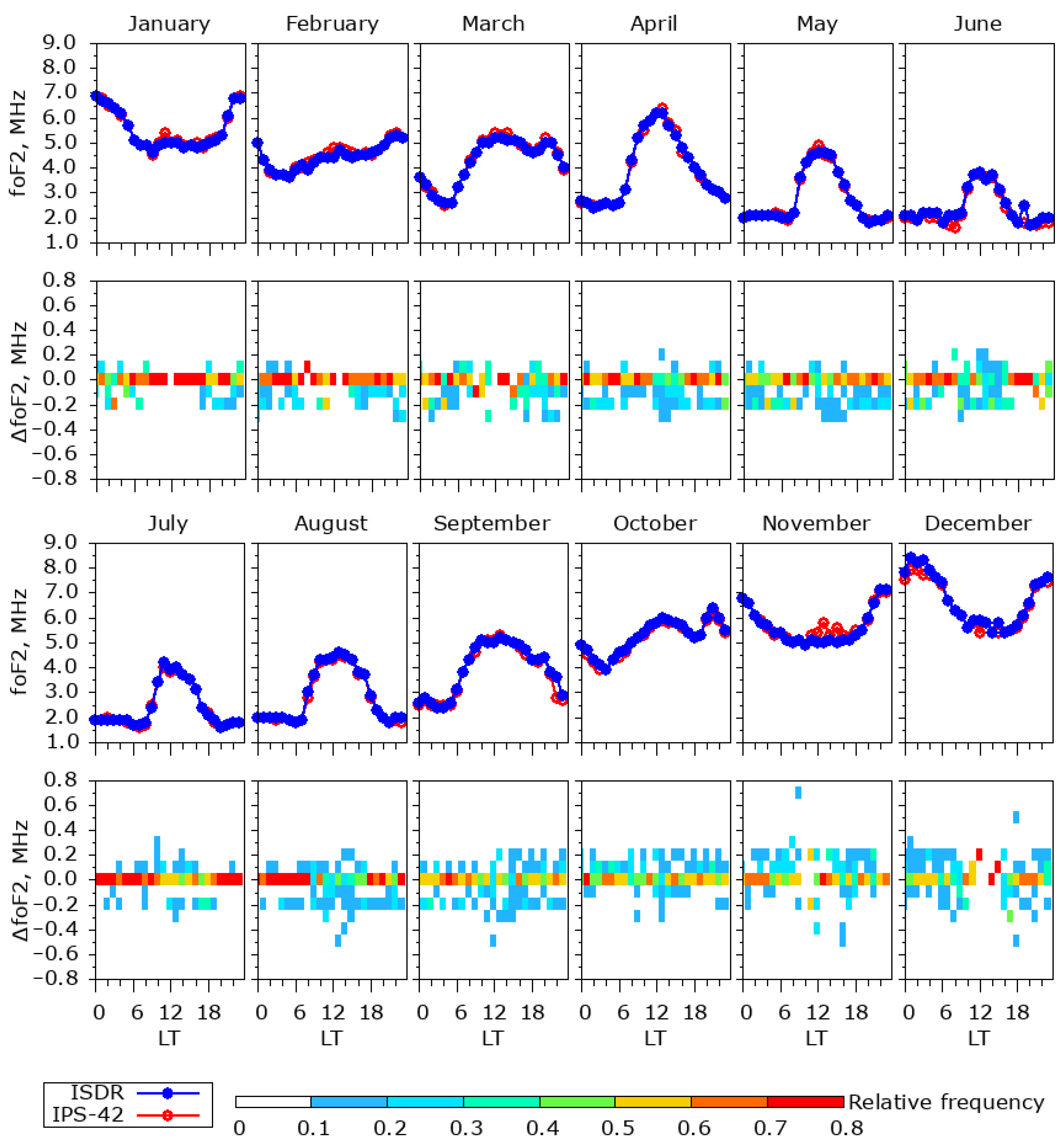
3.2. Methodology and Results of the ISDR and IPS-42 Data Comparison

Two techniques to compare the data of the IPS-42 and ISDR have been used: the direct matching of ionogram images and comparing manually scaled ionospheric parameters. The first technique requires the pre-processing of raw ionogram images due to the different frequencies and height resolutions, as well as the data visualization peculiarities used by the two ionosondes. The IPS-42 uses a hardware-fixed set of frequencies and heights. The ionogram image contains 576 columns and 512 rows that corresponds to the logarithmically spaced frequencies from 1 to 22.6 MHz and linearly spaced virtual heights from 0 to 800 km, respectively. It also contains height and frequency ticks as well as date and local time (LT = UTC—4 h) labels embedded into the image. Every pixel on the image is represented by 1 bit. The operation mode parameters of the ISDR are configurable and can be changed if required. The first three years of the ISDRs operation allowed us to choose an optimal configuration for the UAS. The standard sounding mode for the ISDR uses a 16-bit complementary code and 320 frequencies from 1 to 16 MHz with a frequency step 0.035 MHz below 10 MHz and 0.1 MHz above 10 MHz. The height step is 0.75 km, while the height resolution (determined by the length of one chip) corresponds to 4.5 km. The minimum and maximum heights are 85 km and 820 km, respectively. As was mentioned above, the ISDRs raw ionograms are stored as 2D arrays of the reflected signal amplitude, phase, and Doppler shift, providing more flexibility for post-processing than IPS-42 ionogram images.

The preprocessing of the ionograms is performed with a script written in Python 3 language using libraries such as NumPy, Pillow (PIL Fork), OpenCV-Python, and SciPy. The preprocessing contains the following steps (their results are presented in Figure 6):

-

The removal of interferences using the Non-local Means Denoising algorithm [49]. Additionally, on the IPS-42 ionograms, the frequency and height ticks, as well as date, time, and ionosonde identification number labels, are removed by subtracting manually the created mask from the original image.

-

A bilinear (2D) data interpolation within the same, chosen for both ionosondes, frequency and virtual height ranges. The frequency range of 1–12 MHz and the virtual height range of 100–600 km have been selected. The number of points for each dimension is 512.

-

A data binarization, that is a conversion of an ionogram to a black-and-white image using the selected threshold, so that the ionogram images from different instruments can be compared directly.

Therefore, as a result of preprocessing, a pair of ionograms obtained by two ionosondes at approximately the same time (the difference between the start moments of the soundings does not exceed 1 min) is obtained. The comparison of two ionograms is presented in the form of an image containing the traces shown in three colors. The pixels that are present on the ISDR ionogram only are shown in blue, the IPS-42 only pixels are in red, and the pixels present on both ionograms are in green.

Figure 7 demonstrates some typical examples of the ionogram’s comparison. It can be seen that signal traces obtained by the two ionosondes (green pixels) generally coincide both in the frequencies and virtual heights. At the same time, one can notice that the thickness of the traces is smaller for the ISDR than for the IPS-42. It can be explained by the higher virtual height resolution of the ISDR and the difference in the transfer functions of ionosondes, which can lead to a broadening of the pulses recorded by the IPS-42. It should be noted that the narrower traces obtained by the ISDR are located inside the wider traces registered by the IPS-42. The centers of the traces derived by different ionosondes coincide well, which confirms the correctness of the ISDR data, while the lower edge of the IPS-42 traces is located systematically lower than the corresponding edge of the ISDR. It may lead to the underestimation of the ionospheric layer virtual heights for the IPS-42 compared to the ISDR because the manual scaling procedure employs the lower edge of the traces to determine the layer heights. This feature must be considered when interpreting the scaling results and comparing the ionospheric parameters obtained from the two instruments.

The ionogram comparison images do not allow us to quantitatively estimate the difference between the signal-to-noise ratio of the two instruments and confidently estimate the performance of the new system. In some cases, (for example, the extraordinary component of the traces of the F2 layer in Figure 7a,c and the ordinary and extraordinary components of the traces of the F2 layer in Figure 7b), the length of the traces is longer on the ionograms obtained using the IPS-42 ionosonde (shown in red). In other cases, (for example, the ordinary component of the F2 layer trace in Figure 7c and the extraordinary component of the trace of the F2 layer in Figure 7d), the length of the traces is longer on the ionograms obtained using the ISDR (shown in blue).

In order to perform a statistically meaningful comparison, the performance of the two instruments must be analyzed for the different ionospheric conditions, as a function of the time of the day or season. To perform such an analysis, a second comparison technique is used to compare the long-term arrays of the ionospheric parameters obtained using manually scaled ionograms from both ionosondes. In this study, the comparison of the data, such as the critical frequencies and virtual heights of F2, E, and Es layers during the whole year of 2021 is presented.

Figure 8 shows the distribution of the differences in the critical frequencies ΔfoF2, ΔfoE, and ΔfoEs, as well as virtual heights differences in Δh’F, Δh’E, and Δh’Es measured by the different ionosondes in 2021. In this work, hourly ionograms were analyzed. Therefore, the number of ionograms per year can reach 24 × 365 = 8760. However, the total number of analyzed iongrams is smaller due to a few data gaps. The deviation in the total number of analyzed parameters (ΔfoF2, Δh’F, ΔfoE, Δh’E, ΔfoEs, and Δh’Es) in the presented statistics is caused by the fact that not all ionograms contain traces corresponding to the E, Es, and F layers. Moreover, manual ionogram scaling implies assigning qualifying and descriptive letters to the scaled parameters having certain features in accordance with the rules described in [48]. Only numerical values without descriptive letters (usually indicating a poor data quality) were used in the statistical analysis. Critical frequencies and virtual heights are scaled independently and can have different descriptive letters too. Therefore, the total numbers of the ΔfoF2, ΔfoE, ΔfoEs, Δh’F, Δh’E, and Δh’Es parameters for the selected period are different. The statistical parameters, such as the mean value, standard deviation, maximum and minimum values, and sample size, are presented as well. Hereinafter, the difference in a parameter means its value is obtained from the IPS-42 subtracted from the value derived from the ISDR. Figure 8a–c depicts the distributions of the differences in the critical frequencies of the F2, E, and Es layers, respectively. All the distributions are quite symmetric, with peak values very close to zero, which means the absence of a systematic shift in the foF2, foE, and foEs values observed by the two instruments. The distribution peaks are quite sharp, with the standard deviation (STD) of 0.11 MHz for ΔfoF2, 0.15 MHz for ΔfoE, and 0.21 MHz for ΔfoEs. Thus, both ionosondes demonstrate a good agreement in determining the critical frequencies with the similar accuracy for the F, E, and Es layers. Figure 8d–f shows the similar distributions of the differences in the virtual heights for the F, E, and Es layers. Unlike the critical frequencies, the distributions in the virtual height differences demonstrate the small positive shift of 1.38 km, 4.29 km, and 5.85 km for the F, E, and Es layers’ virtual heights, respectively. Therefore, the IPS-42 systematically underestimates the height of the ionospheric layers compared to the ISDR that was detected earlier while matching the ionograms obtained by the two instruments. It should be noted that the revealed differences in the height for all the ionospheric layers are quite small and are comparable with the height resolution of the ISDR (~4 km), IPS-42 (~6 km), and the scaling software (5 km). The STD value of Δh’F is greater than that of Δh’E and Δh’Es, which can be explained by the higher dynamics of the F layer, taking into account that the two instruments do not perform soundings at exactly the same time.

As the most important parameter obtained from the ionograms is the critical frequency of the F2 layer (foF2), the accuracy of deriving this parameter using the ISDR was studied in detail. Figure 9 shows the distributions of ΔfoF2 similar to those presented in Figure 8a but which are calculated for every month of 2021. Similar to Figure 8a, the peaks of all the distributions are close to zero, meaning the absence of a systematic shift in the foF2 values observed by both ionosondes for every month of the year. The STD does not exceed 0.15 MHz during the whole year. The minimal values of STD (0.09 MHz and less) are observed from January to July, while the months from August to December are characterized by the STD from 0.11 MHz to 0.15 MHz. The distributions for the second part of the year also demonstrate the largest minimum and maximum values of the difference. The worst agreement between the foF2 values derived from IPS-42 and ISDR ionograms was observed for November (STD = 0.14 MHz, MAX − MIN = 1.3 MHz) and December (STD = 0.15 MHz, MAX − MIN = 1.3 MHz). We analyzed the ionogram images for these two months in more detail and found out that the large difference in the foF2 values is associated with the poor quality of the ionograms obtained using the IPS-42 during this period.

In addition to the analysis of the seasonal behavior of ΔfoF2, the diurnal variations in the median foF2 values have been considered. The distributions similar to those shown in Figure 8a and Figure 9 but calculated for each hour during the whole year of 2021 are presented in Figure 10.

One can see that the diurnal variations in the median values of the critical frequency foF2 are very similar for both ionosondes throughout the year. A greater spread of the differences in the critical frequency ΔfoF2 (corresponding to the greater difference in the median values of foF2) are observed in November and December 2021. This is consistent with the result of the analysis of the monthly distributions presented earlier and may be associated with the poor quality of the ionograms obtained by IPS-42. It can be explained by a combination of several factors, such as the seasonal fluctuation in the absorption level in the ionosphere, the hardware features of both ionosondes, such as the sounding pulse length and shape, and the signal processing in the IPS-42 that employs analog and digital circuits containing nonlinear amplifiers, integration, and subtraction of the transmitted wave form from the received signal (see [28] for more details). Figure 11 demonstrates the better quality of the ISDR ionograms (Figure 11b,d,f) compared to the corresponding IPS-42 ones (Figure 11a,c,e) for the random date of 28 December 2021. One can see that the F layer traces on the ionograms obtained by the IPS-42 are always shorter than on the ionograms obtained by the ISDR. All ionograms obtained by the IPS-42 and ISDR in 2021 are given in the additional materials (see Data Availability Statement section).

The inverted diurnal variations of the foF2 parameter (maximum at nighttime instead of noon) is attributed to what is called the “Weddell Sea Anomaly” [50,51]. It can be related to the distribution of the thermospheric winds [52] or the effects of the tidal and stationary planetary waves [53].

4. Discussion

Turning to the discussion of the comparison of the ionograms obtained with the SDR-based and the conventional (IPS-42 in this case) ionosondes, it is important to underline that the developed ISDR has been operating accident-free in Antarctica for five years. Since its installation at the UAS in April 2017, the ISDR has never required specific maintenance or repairs. Only a few software updates and optimizations of the working schedule have been performed. The regular maintenance according to the standard IPS-42 protocol was performed for the antenna feeder system solely, which is shared by both devices. Therefore, the result of this study is not only the analysis of the accuracy of the ionograms, but also a confirmation of the reliability of the ISDR. It should also be noted that the comparison of the performance of the two instruments was done for the basic configuration of the ISDR. The enhanced passive ISDR installed at the UAS in 2022 allows for the distinguishing of the O- and X- traces of different propagation modes on the ionograms. In addition, it provides the higher quality of the ionograms due to a lower level of local interference. Furthermore, an important result is the confirmation of the possibility to obtain oblique ionograms in the passive mode onboard a marine vessel while it is sailing at distances up to 1,400 km from the active ionosonde.

The accuracy of determining the ionospheric characteristics by the ISDR was analyzed both by direct matching of the ionogram images and by comparing the ionospheric parameters calculated by manual scaling ionograms using the same software package. The observation data during the whole year of 2021 were analyzed. The comparison of the ionogram images demonstrated the coincidence of the traces of all ionospheric layers, both in the frequency and in the virtual height. Similar results were also obtained when comparing the virtual heights of the F, E, and Es layers for the whole period of the observations. The distributions of the height differences obtained from different ionosondes indicate an underestimation of the layer heights obtained by the IPS-42 compared to the ISDR. This effect may be attributed to the lower height resolution of the IPS-42 ionograms and the difference in the transfer functions of the ionosondes. When estimating the critical frequency of the ionospheric layers, this effect does not appear because both ionosondes have a similar frequency resolution. For all layers, the distributions of the critical frequency differences demonstrate close to zero mean values. This can be interpreted as proof of the validity of the ISDR data. When comparing a long-term data series, special attention was paid to the main ionospheric parameter obtained from the ionograms: the critical frequency of the F2 layer (foF2). The analysis of the distribution of the differences in the foF2 (ΔfoF2) has shown the good correspondence of the data obtained by the two instruments throughout the year. Additionally, the diurnal time series of the median values of the foF2 obtained by the two instruments matched well during each month of the year. Therefore, the performance of the ISDR was confirmed using a statistically meaningful set of data.

The comparison of the ionogram images showed the generally comparable performance of the two ionosondes in terms of the presence of ionospheric traces. At the same time, the ranges of the heights and frequencies or ionospheric conditions, under which one ionosonde has an advantage over another and vice versa, have not been identified. It should be noted that the performed comparison cannot be considered to be comprehensive, since the performance of the IPS-42 is achieved by a higher radiation power, while the ISDR makes use of the pulse compression and coherent averaging to achieve similar signal-to-noise ratio levels. Therefore, the duration of the ISDR sounding is an order of magnitude longer than that of the IPS-42. As a result, during the time from the beginning of the IPS-42 sounding to the end of the ISDRs operation, the shape of the signal trace may change based on the ionospheric dynamics. An equivalent comparison of the two instruments is possible if the ISDR sounding time or, alternatively, the IPS-42 radiation power is reduced significantly. The future work considered by the authors is to use a more powerful amplifier for the ISDR instead of IC-718, which will make it possible to study highly dynamic ionospheric processes and to take out of the service IPS-42. Another promising option is creating a network of passive ISDRs located at distances from several tens to several hundred kilometers from the active ISDR. Similar measurements, but performed using continuous wave (CW) signals, previously performed at the UAS made it possible to monitor the characteristics of travelling ionospheric disturbances (TIDs) over the Antarctic Peninsula [54,55]. Expanding the network of SDR-based ionosondes can significantly improve the understanding of the TID dynamics in the region.

5. Conclusions

The most important practical result of this study is the comparison of the performance of an SDR-based ionosonde with a reference IPS-42 instrument carried out for the first time using a long-term data set. The comparison shows that the developed low-cost, low-power SDR-based ionosonde has demonstrated an equivalent or higher level of performance compared to the more expensive conventional ionosonde in terms of the reliability, flexibility, and accuracy of determining the main ionospheric parameters. In some characteristics (for example, in virtual height resolution and the ability to provide polarization information), the ISDR is superior to the IPS-42 ionosonde used for a comparison in this study. The main disadvantage of the ISDR in its actual hardware configuration is the significantly longer sounding time, which limits the application of the ISDR to study fast ionospheric processes.

The advantages of SDR-based ionosondes in comparison with their conventional counterparts and the possibilities for their application arising from these advantages are summarized below.

Low-cost. The cost of the components for the basic configuration of the ionosonde installed at the UAS (without the cost of the antenna feeder system) is less than USD 5000. Similar cost estimates are given in the literature for other prototypes of SDR-based ionosondes [21,22,23]. The cost of mass-produced ionosondes such as CADI and DPS4D exceeds this amount by an order of magnitude or more.

Scalability. Using two RX channels of the base configuration ISDR, which are fed from two orthogonal linearly polarized antennas, allows for polarization measurements and discriminating different propagation modes in ionogram traces. Two USRP N200 kits can be converted into a fully fledged four channel coherent receiver using a USRP MIMO cable [56]. Such a system allows for measuring the angles of arrival of the signal, as well as reconstructing the drift velocity of the plasma using the method of Doppler interferometry [57]. As the IC-718 transceiver is used only as a power amplifier, it can be replaced with a more powerful device with a minimal software and hardware modifications. In such a case, the sounding time can be significantly reduced by only changing one software configuration setting.

Networking. The possibility of building a network of active and passive ionosondes using enhanced configurations of ISDRs has been confirmed by the long-term simultaneous operation of active and passive ISDRs. The feasibility study of the system performed onboard of the RV “Noosfera” showed that the system with its current configuration can be effectively used on distances up to 1400 km as well as on moving platforms.

Based on the above-described advantages, the scope of the application of the SDR-based ionosondes can be as follows:

-

Equipping a large number of geophysical observatories with passive SDR-based ionosondes. In particular, when using passive devices, ionosondes can be installed at observatories where, due to problems with the electromagnetic compatibility, the installation of active devices is prohibitive.

-

Building regional networks of ionosondes, which can be used to study the ionospheric dynamics, such as TIDs, and provide support to operational systems, such as JORN. Until now, similar studies have been implemented using spaced HF receivers operating in the CW mode [54,55,58,59] or the sparse networks of ionosondes [60,61]. However, for the detailed diagnostics of TIDs using ionosondes, the spacing between observation points must be comparable with the wavelengths of the disturbances, i.e., a few hundred kilometers or less. The regional networks of the SDR-based ionosondes, in which a large number of passive units are located around several active devices, can significantly increase the information content of the monitoring of the inhomogeneous structure of the ionosphere. The joint use of ionosonde networks and existing dense networks of GNSS receivers can further improve the capabilities of the ionospheric modelling and diagnostics.

-

Standard data formats provided by SDR-based ionosondes and the flexibility of their operation modes facilitates the development of ionogram autoscaling programs. For example, such a program based on an artificial neural network for the analysis of the ionograms obtained using the IPS-42 and ISDR installed at the UAS is under development [62]. The availability of ionograms for more than 30 years of observations at the UAS and the results of their manual scaling provide a great opportunity for the implementation of ionospheric models using machine learning techniques.

-

It is not difficult to adapt the SDR-based ionosondes to local ionospheric conditions due to their low-cost and ease of deployment. For example, it is possible to create ionosondes and networks of ionosondes in the polar regions, at the equator and near heating facilities [63,64], where it is important to track highly dynamic ionospheric processes.

References

1. Appleton, E.V.; Barnett, M.A.F. Local reflections of wireless waves from the upper atmosphere. Nature 1925, 25, 333–334. [Google Scholar] [CrossRef]
2. Breit, G.; Tuve, M.A. A Test of the Existence of the Conducting Layer. Phys. Rev. 1926, 28, 554–575. [Google Scholar] [CrossRef]
3. Gilliland, T.R. Ionospheric investigations. Nature 1934, 134, 379. [Google Scholar] [CrossRef]
4. Bibl, K. Evolution of the ionosonde. Ann. Geophys. 1998, 41, 667–680. [Google Scholar] [CrossRef]
5. Bibl, K.; Reinisch, B.W. The universal digital ionosonde. Radio Sci. 1978, 13, 519–530. [Google Scholar] [CrossRef]
6. Reinisch, B.W.; Galkin, I.A.; Khmyrov, G.M.; Kozlov, A.V.; Bibl, K.; Lisysyan, I.A.; Cheney, G.P.; Huang, X.; Kitrosser, D.F.; Paznukhov, V.V.; et al. New Digisonde for research and monitoring applications. Radio Sci. 2009, 44, RS0A24. [Google Scholar] [CrossRef]
7. Themens, D.; Reid, B.; Elvidge, S. ARTIST ionogram autoscaling confidence scores: Best practices. URSI Radio Sci. Lett. 2022, 4, 1–5. [Google Scholar] [CrossRef]
8. Reinisch, B.W.; Galkin, I.A. Global Ionospheric Radio Observatory (GIRO). Earth Planets Space 2011, 63, 377–381. [Google Scholar] [CrossRef] [Green Version]
9. Gao, S.; MacDougall, J.W. A dynamic ionosonde design using pulse coding. Can. J. Phys. 1992, 69, 1184–1189. [Google Scholar] [CrossRef]
10. Wright, J.W.; Pitteway, M.L.V. Real-time acquisition and interpretation capabilities of the Dynasonde 2. Determination of magnetoionic mode and echolocation using a small spaced receiving array. Radio Sci. 1979, 14, 827–835. [Google Scholar] [CrossRef]
11. Zuccheretti, E.; Tutone, G.; Sciacca, U.; Bianchi, C.; Baskaradas, J.A. The new AIS-INGV digital ionosonde. Ann. Geophys. 2003, 46, 647–659. [Google Scholar] [CrossRef]
12. Chen, G.; Zhao, Z.; Li, S.; Shi, S. WIOBSS: The Chinese low-power digital ionosonde for ionospheric backscattering detection. Adv. Space Res. 2009, 43, 1343–1348. [Google Scholar] [CrossRef]
13. Huang, S.; Zhao, Z.; Yang, G.; Chen, G.; Li, T.; Li, N.; Yang, J. A new design of low-power portable digital ionosonde. Adv. Space Res. 2013, 51, 388–394. [Google Scholar] [CrossRef]
14. Szwabowski, M.; Dziak-Jankowska, B.; Pożoga, M.; Tomasik, Ł. The 2009–2012 Ionosonde and IRI2012 Variability of foF2, hmF2, M3000F2, B0, B1 Parameters over Warsaw. Acta Geophys. 2016, 64, 1211–1223. [Google Scholar] [CrossRef] [Green Version]
15. Rideout, W.; Coster, A. Automated GPS processing for global total electron content data. GPS Solut. 2006, 10, 219–228. [Google Scholar] [CrossRef]
16. Vierinen, J.; Coster, A.J.; Rideout, W.C.; Erickson, P.J.; Norberg, J. Statistical framework for estimating GNSS bias. Atmos. Meas. Tech. Discuss. 2015, 8, 9373–9398. [Google Scholar] [CrossRef] [Green Version]
17. Ferreira, A.A.; Borges, R.A.; Paparini, B.; Ciraolo, L.; Radicella, S.M. Short-term estimation of GNSS TEC using a neural network model in Brazil. Adv. Space Res. 2017, 60, 1765–1776. [Google Scholar] [CrossRef]
18. Nie, Y. A Software Radio Based Ionosonde Using GNU Radio; Western University: London, ON, Canada, 2011; pp. 1–99. Available online: https://ir.lib.uwo.ca/digitizedtheses/3254 (accessed on 1 December 2022).
19. Vierinen, J. On Statistical Theory of Radar Measurements. A Dissertation for the Degree of Doctor of Science, Aalto University, Espoo, Finland, 2012. [Google Scholar]
20. Mendoza, J.J.B.; Ruiz, C.F.Q.; Jaramillo, C.R.P. Implementation of an Electronic Ionosonde to Monitor the Earth’s Ionosphere via a Projected Column through USRP. Sensors 2017, 17, 946. [Google Scholar] [CrossRef] [Green Version]
21. Floer, M. Design and Implementation of a Software Defined Ionosonde; The Arctic University of Norway: Tromsø, Norway, 2020; Available online: https://munin.uit.no/bitstream/handle/10037/19423/thesis.pdf?sequence=2&isAllowed=y (accessed on 1 December 2022).
22. Software Defined Radio Ionosonde. Available online: https://github.com/jvierine/ionosonde (accessed on 15 July 2022).
23. Shindin, A.V.; Moiseev, S.P.; Vybornov, F.I.; Grechneva, K.K.; Pavlova, V.A.; Khashev, V.R. The Prototype of a Fast Vertical Ionosonde Based on Modern Software-Defined Radio Devices. Remote Sens. 2022, 14, 547. [Google Scholar] [CrossRef]
24. Galkin, I.A.; Reinisch, B.W.; Osokov, G.A.; Zazobina, E.G.; Neshyba, S.P. Feedback neural networks for ARTIST ionogram processing. Radio Sci. 1996, 31, 1119–1128. [Google Scholar] [CrossRef]
25. Galkin, I.A.; Reinisch, B.W. The new ARTIST 5 for all digisondes. INAG Bull. 2008, 69, 1–8. [Google Scholar]
26. Scotto, C.; Pezzopane, M. Software for the automatic scaling of critical frequency f0F2 and MUF(3000)F2 from ionograms applied at the Ionospheric Observatory of Gibilmanna. Ann. Geophys. 2004, 47, 1783–1790. [Google Scholar] [CrossRef]
27. Scotto, C.; Pezzopane, M. The INGV software for the automatic scaling of foF2 and MUF(3000)F2 from ionograms: A performance comparison with ARTIST 4.01 from Rome data. J. Atmos. Sol. -Terr. Phys. 2005, 67, 1063–1073. [Google Scholar] [CrossRef]
28. Broom, S.M. A new ionosonde for Argentine Islands ionospheric observatory, Faraday Station. Br. Antarct. Surv. Bull. 1984, 62, 1–6. Available online: http://nora.nerc.ac.uk/id/eprint/523821/ (accessed on 15 July 2022).
29. Zalizovski, A.; Koloskov, O.; Kashcheyev, A.; Kashcheyev, S.; Yampolski, Y.; Charkina, O. Doppler vertical sounding of the ionosphere at the Akademik Vernadsky station. Ukr. Antarct. J. 2020, 1, 56–68. [Google Scholar] [CrossRef]
30. Zalizovski, A.V.; Kashcheyev, A.S.; Kashcheyev, S.B.; Koloskov, A.V.; Lisachenko, V.N.; Paznukhov, V.V.; Pikulik, I.I.; Sopin, A.A.; Yampolski, Y.M. A prototype of a portable coherent ionosonde. Space Sci. Technol. 2018, 24, 10–22. (In Russian) [Google Scholar] [CrossRef]
31. Koloskov, O.; Kashcheyev, A.; Zalizovski, A.; Kashcheyev, S.; Lisachenko, V.; Bogomaz, O. Results of Vertical Ionospheric Sounding at the Ukrainian Antarctic Station Akademik Vernadsky. In Proceedings of the 3rd URSI AT-AP-RASC, Gran Canaria, Spain, 29 May–3 June 2022. [Google Scholar] [CrossRef]
32. USRP N200 Software Defined Radio (SDR). Available online: https://www.ettus.com/all-products/un200-kit/ (accessed on 15 July 2022).
33. LFTX Daughterboard 0-30 MHz Tx. Available online: https://www.ettus.com/all-products/lftx/ (accessed on 15 July 2022).
34. LFRX Daughterboard 0-30 MHz Rx. Available online: https://www.ettus.com/all-products/lfrx/ (accessed on 15 July 2022).
35. ZX80-DR230+. Available online: https://www.minicircuits.com/pdfs/ZX80-DR230+.pdf (accessed on 15 July 2022).
36. IC-718 HF All Band Transceiver. Available online: https://www.icomamerica.com/en/products/amateur/hf/718/default.aspx (accessed on 15 July 2022).
37. Mean Well Sp-200-13.5. Available online: https://www.meanwell-web.com/en-gb/ac-dc-single-output-enclosed-power-supply-with-pfc-sp--200--13.5 (accessed on 15 July 2022).
38. UHD (USRP Hardware Driver™). Available online: https://www.ettus.com/sdr-software/uhd-usrp-hardware-driver/ (accessed on 15 July 2022).
39. Schmidt, G.; Ruster, R.; Czechowsky, P. Complementary code and digital filtering for detection of weak VHF radar signals from the mesosphere. IEEE Trans. Geosci. Electron. 1979, 17, 154–161. [Google Scholar] [CrossRef]
40. GPSDO Kit for USRP N200/N210. Available online: https://www.ettus.com/all-products/gpsdo-kit/ (accessed on 15 July 2022).
41. Earl, G.F.; Ward, B.D. The frequency management system of the Jindalee over-the-horizon backscatter HF radar. Radio Sci. 1987, 22, 275–291. [Google Scholar] [CrossRef]
42. JINDALEE Operational Radar Network. Available online: https://www.dst.defence.gov.au/innovation/jindalee-operational-radar-network (accessed on 15 July 2022).
43. Wilkinson, P.; Kennewell, J.A.; Cole, D. The development of the Australian Space Forecast Centre (ASFC). Hist. Geo Space. Sci. 2018, 9, 53–63. [Google Scholar] [CrossRef] [Green Version]
44. Koloskov, O.V.; Kashcheyev, A.S.; Zalizovski, A.V.; Kashcheyev, S.B.; Budanov, O.V.; Charkina, O.V.; Pikulik, I.I.; Lysachenko, V.M.; Sopin, A.O.; Reznychenko, A.I. New Digital Ionosonde Developed for Ukrainian Antarctic Station “Akademik Vernadsky”. In Proceedings of the IX International Antarctic Conference Dedicated to the 60th Anniversary of the Signing of the Antarctic Treaty in the Name of Peace and Development of International Cooperation: Physical Sciences, Kyiv, Ukraine, 14–16 May 2019. [Google Scholar]
45. Koloskov, O.; Kashcheyev, A.; Zalizovski, A.; Bogomaz, O. Low-Cost SDR-Based Ionosondes as a Tool for Geospace Research. In Proceedings of the 21st International Beacon Satellite Symposium, Boston, MA, USA, 1–5 August 2022. [Google Scholar]
46. Bogomaz, O.V.; Shulha, M.O.; Kotov, D.V.; Zhivolup, T.G.; Koloskov, A.V.; Zalizovski, A.V.; Kashcheyev, S.B.; Reznychenko, A.I.; Hairston, M.R.; Truhlik, V. Ionosphere over Ukrainian Antarctic Akademik Vernadsky station under minima of solar and magnetic activities, and daily insolation: Case study for June 2019. Ukr. Antarct. J. 2019, 2, 84–93. [Google Scholar] [CrossRef]
47. Reznychenko, M.; Bogomaz, O.; Kotov, D.; Zhivolup, T.; Koloskov, O.; Lisachenko, V. Observation of the ionosphere by ionosondes in the Southern and Northern hemispheres during geospace events in October 2021. Ukr. Antarct. J. 2022, 20, 18–30. [Google Scholar] [CrossRef]
48. Wakai, N.; Ohyama, H.; Koizumi, T. Manual of Ionogram Scaling Third Version; Radio Research Laboratory Ministry of Posts and Telecommunications: Tokyo, Japan, 1987. Available online: https://www.sws.bom.gov.au/IPSHosted/INAG/scaling/japanese_manual_v3.pdf (accessed on 24 December 2022).
49. Buades, A.; Coll, B.; Morel, J.M. Non-local means denoising. Image Process. Online 2011, 1, 208–212. [Google Scholar] [CrossRef] [Green Version]
50. Bellchambers, W.H.; Piggott, W.R. Ionospheric Measurements Made at Halley Bay. Nature 1958, 182, 1596–1597. [Google Scholar] [CrossRef]
51. Dudeney, J.R.; Piggott, W.R. Antarctic Ionospheric Research. In Upper Atmosphere Research in Antarctica; Lanzerotti, L.J., Park, C.G., Eds.; AGU: Washington, DC, USA, 1978; Volume 29, pp. 200–235. [Google Scholar] [CrossRef]
52. Kohl, H.; King, J.W. Atmospheric winds between 100 and 700 km and their effects on the ionosphere. J. Atmos. Terr. Phys. 1967, 29, 1045–1062. [Google Scholar] [CrossRef]
53. Chang, L.C.; Liu, H.; Miyoshi, Y.; Chen, C.; Chang, F.; Lin, C.; Liu, J.; Sun, Y. Structure and origins of the Weddell Sea Anomaly from tidal and planetary wave signatures in FORMOSAT-3/COSMIC observations and GAIA GCM simulations. J. Geophys. Res. Space Phys. 2015, 120, 1325–1340. [Google Scholar] [CrossRef]
54. Galushko, V.G.; Kashcheyev, A.S.; Kashcheyev, S.B.; Koloskov, A.V.; Pikulik, I.I.; Yampolski, Y.M.; Litvinov, V.A.; Milinevsky, G.P.; Rakusa-Suszczewski, S. Bistatic HF diagnostics of TIDs over the Antarctic Peninsula. J. Atmos. Sol. -Terr. Phys. 2007, 69, 403–410. [Google Scholar] [CrossRef]
55. Paznukhov, V.V.; Sopin, A.A.; Galushko, V.G.; Kashcheyev, A.S.; Koloskov, A.V.; Yampolski, Y.M.; Zalizovski, A.V. Occurrence and characteristics of Traveling Ionospheric Disturbances in the Antarctic Peninsula region. J. Geophys. Res. Space Phys. 2022, 127, e2022JA030895. [Google Scholar] [CrossRef]
56. MIMO Cable. Available online: https://www.ettus.com/all-products/mimo-cbl/ (accessed on 15 July 2022).
57. Bibl, K.; Pfister, W.; Reinisch, B.W.; Sales, G.S. Velocities of small and medium scale ionospheric irregularities deduced from Doppler and arrival angle measurements. Space Res. 1975, 15, 405–411. [Google Scholar]
58. Lastovicka, J.; Chum, J. A review of results of the international ionospheric Doppler sounder network. Adv. Space Res. 2017, 60, 1629–1643. [Google Scholar] [CrossRef]
59. Zalizovski, A.V.; Yampolski, Y.M.; Mishin, E.; Kashcheyev, S.B.; Sopin, A.O.; Koloskov, A.V.; Lisachenko, V.N.; Reznychenko, A.I. Multi-position facility for HF Doppler sounding of ionospheric inhomogeneities in Ukraine. Radio Sci. 2021, 56, e2021RS007303. [Google Scholar] [CrossRef]
60. Verhulst, T.; Altadill, D.; Mielich, J.; Reinisch, B.; Galkin, I.; Mouzakis, A.; Belehaki, A.; Burešová, D.; Stankov, S.; Blanch, E.; et al. Vertical and oblique HF sounding with a network of synchronised ionosondes. Adv. Space Res. 2017, 60, 1644–1656. [Google Scholar] [CrossRef]
61. Reinisch, B.; Galkin, I.; Belehaki, A.; Paznukhov, V.; Huang, X.; Altadill, D.; Buresova, D.; Mielich, J.; Verhulst, T.; Stankov, S.; et al. Pilot ionosonde network for identification of traveling ionospheric disturbances. Radio Sci. 2018, 53, 365–378. [Google Scholar] [CrossRef]
62. Bogomaz, O.; Shulha, M.; Kotov, D.; Koloskov, A.; Zalizovski, A. An artificial neural network for analysis of ionograms obtained by ionosonde at the Ukrainian Antarctic Akademik Vernadsky station. Ukr. Antarct. J. 2020, 2, 59–67. [Google Scholar] [CrossRef]
63. Stubbe, P.; Kopka, H.; Lauche, H.; Rietveld, M.T.; Brekke, A.; Holt, O.; Jones, T.B.; Robinson, T.; Hedberg, A.; Thidé, B.; et al. Ionospheric modification experiments in northern Scandinavia. Atmos. Terr. Phys. 1982, 44, 1025–1041. [Google Scholar] [CrossRef]
64. Bailey, P.G.; Worthington, N.C. History and Applications of HAARP Technologies: The High Frequency Active Auroral Research Program. Volume 2: Electrochemical Technologies, Conversion Technologies and Thermal Management. In Proceedings of the Thirty-Second Intersociety Energy Conversion Engineering Conference, Honolulu, HI, USA, 27 July–1 August 1997; pp. 1317–1322. [Google Scholar] [CrossRef]
Figure 1. Block diagram of the ionosonde. Light gray blocks (GPSDO and receiving channel B) are optional for the base configuration and are used in the extended configuration.
Atmosphere 14 00159 g001
Figure 2. (a) Phase difference distribution and (b) ionogram (phase difference color coded) obtained using ISDR at the “Akademik Vernadsky” station on 7 October 2022. Additional information can be found in Supplementary Materials.
Atmosphere 14 00159 g002
Figure 3. Schematic diagram of antenna connections.
Atmosphere 14 00159 g003
Figure 4. Antenna system of passive ionosonde at UAS.
Atmosphere 14 00159 g004
Figure 5. (a) Ionogram at UAS and (b) ionogram onboard the RV “Noosfera” (coordinates: 60.398532° S, 58.403656° W; distance: ~615 km) obtained on 28 March 2022 at 18:26 LT (LT = UT—4h). Additional information can be found in Supplementary Materials.
Atmosphere 14 00159 g005
Figure 6. (a) The original ionogram obtained by IPS-42 on 2 December 2018 at 05:45 LT, (b) the result of noise, ticks, and labels removal, (c) the result of interpolation and binarization. Additional information can be found in Supplementary Materials.
Atmosphere 14 00159 g006
Figure 7. (a) Ionogram comparison images obtained at UAS by ISDR and IPS-42 on 12 April 2021 at 07:45 LT, (b) 6 May 2021 at 13:15 LT, (c) 4 May 2021 at 15:30 LT, and (d) 9 November 2021 at 23:00 LT. Pixels present on ISDR ionograms only are shown in blue, on IPS-42 ionograms only—in red, on both ionograms—in green. Additional information can be found in Supplementary Materials.
Atmosphere 14 00159 g007
Figure 8. Distribution of the differences in critical frequencies (a) ΔfoF2, (b) ΔfoE, (c) ΔfoEs and virtual heights (d) Δh’F, (e) Δh’E, (f) Δh’Es for the 2021. Additional information can be found in Supplementary Materials.
Atmosphere 14 00159 g008
Figure 9. Distribution of the differences in critical frequency ΔfoF2 by month during the 2021.
Atmosphere 14 00159 g009
Figure 10. Median values of the critical frequency foF2 (ISDR data—blue lines, IPS-42 data—red lines) and the distribution of diurnal differences in the critical frequency ΔfoF2 for all months of the year 2021.
Atmosphere 14 00159 g010
Figure 11. Ionograms obtained on 28 December 2021 at: 07:00 LT (a) by IPS-42, (b) by ISDR; 16:00 LT (c) by IPS-42, (d) by ISDR; 23:00 LT, (e) by IPS-42, (f) by ISDR.
Atmosphere 14 00159 g011
Disclaimer/Publisher’s Note: The statements, opinions and data contained in all publications are solely those of the individual author(s) and contributor(s) and not of MDPI and/or the editor(s). MDPI and/or the editor(s) disclaim responsibility for any injury to people or property resulting from any ideas, methods, instructions or products referred to in the content.