Early Warning Signals of Dry-Wet Transition Based on the Critical Slowing Down Theory: An Application in the Two-Lake Region of China

Abstract

In recent years, the dry-wet transition (DWT), which often leads to regional floods and droughts, has become increasingly frequent in the Poyang Lake basin and the Dongting Lake basin (hereinafter referred to as the two-lake region). This study aims to investigate the early warning signals (EWSs) for DWT events. Firstly, based on the standardized precipitation index (SPI) at 161 meteorological stations in the two-lake region from 1961 to 2020, the two-lake region is divided into four sub-regions by the Rotational Empirical Orthogonal Function (REOF) analysis method. Then, the occurrence time of the DWT events in each sub-region is determined by the moving t-test (MTT) technique. Finally, by using two indicators (variance and the auto-correlation coefficient) to describe the critical slowing down (CSD) phenomenon, the EWSs denoting the DWT events in all sub-regions are investigated. The results reveal that there was a significant dry-to-wet (wet-to-dry) event around 1993 (2003) in the two-lake region during the last 60 years. The phenomenon of CSD, where the auto-correlation coefficient and variance increases are found in all sub-regions around 10 years before the DWT, suggests that it can be taken as an EWS for the DWT events. This study confirms the effectiveness of applying the slowing down theory in investigating the EWSs for abrupt changes in the two-lake region, aiming to provide a theoretical basis for effective prevention and mitigation against disasters in this region. Moreover, it is expected to be well-applied to the middle and lower reaches of the Yangtze River.

1. Introduction

The Poyang Lake basin and the Dongting Lake basin (hereinafter referred to as the two-lake region) are situated in the middle reaches of the Yangtze River, which covers Jiangxi and Hunan Provinces. Historical records reveal that the two-lake region has long suffered from drought and floods [1]. Specifically, since the middle of the 20th century, floods and drought have become more frequent in the two-lake region due to global warming. In addition, the dry-wet transition (DWT) has become increasingly frequent [2,3]. In general, the time that the climatic system maintains a drought or flood state in the two−lake region is becoming shorter; i.e., the cycle of the transition between dry and wet states has significantly shortened [1,4,5]. This is the key to study the DWT for disaster prevention and reduction.

DWT events include the dry-wet transition and the wet-dry transition, which are typical precipitation anomaly events. Compared with a drought or flood event, the DWT usually causes serious problems, such as regional floods and droughts [6]. Many scholars have carried out a large number of studies on dry-wet transition events. For example, Wu et al. [7] studied the circulation characteristics of DWT events in the middle and lower reaches of the Yangtze River. Li et al. [8] analyzed the DWT characteristics in the Poyang Lake region. Li and Fu [9] used the ECMWF re-analysis data to study the characteristics of atmospheric and surface fluxes before and after the DWT in the Amazon region. Espinoza et al. [10] studied the atmospheric circulation characteristics of DWT events in South America. However, there are few studies on the early warning signals of DWT events. If efficient early warnings can be issued ahead of the DWT, the related departments of the local government should have enough time to take effective measures to reduce the disaster losses. Therefore, it is of great importance to improve the forecast of and early warning system for the DWT in the two-lake region.

However, as complex nonlinear processes are involved in the DWT, existing climate models have limited capabilities in predicting possible DWTs [11,12,13,14]. Nowadays, for the regional drought-flood events caused by the DWT, the prediction studies are mainly based on numerical models, and they mainly focus on the external forcings (sea temperature, sea ice, etc.). However, it is sometimes difficult for numerical models to predict the DWT events. For example, some scholars have revealed that the predictions for the two-lake region are almost contrary to the observational facts in 1999 and 2007 [15,16]. It is a long-term challenge for meteorological departments to accurately predict the regional drought or flood events caused by the DWT. The transition of the climate system between different states is considered as a tipping point. Scheffer et al. proposed a novel method to study the tipping point by using critical slowing down phenomenon [17,18]. This phenomenon can be found in a wide range of fields in nature and human society [19,20], often leading to catastrophic consequences, such as the decline of civilizations or the fall of dynasties caused by abrupt climate changes [21,22]. Hence, it is quite necessary to research the EWSs for the critical transition of nonlinear systems and the possible mechanisms involved.

In the early 21st century, scholars revealed that the CSD theory has remarkable potential for studying EWSs [17,23,24]. In statistical physics, the CSD theory is a concept describing the phenomenon of the dispersed fluctuations formed by the phase transition of a dynamical system. According to the mathematical derivation, the CSD phenomenon is often featured by slower recovery rates from disturbances, an increasing variation amplitude of factors, a reduced ability to return to an old phase, and a prolonged duration of fluctuations [25]. Based on a study of multiple real systems such as the climate system, ecosystem, and medicine, Scheffer et al. [17] proposed that when a system comes close to the tipping point, a CSD phenomenon will occur, which is characterized by a slower recovery rate and increases in the auto-correlation coefficient and variance after the perturbation of the dynamic system. This offers a new direction for exploring the EWSs that indicate the drastic changes in complex systems. By processing the radon concentration in water data using the CSD theory, Yan et al. [26] revealed the appearance of the CSD phenomenon before the Wenchuan earthquake in China in 2008. Recently, some researchers [27,28,29,30,31] have adopted the CSD theory to apply to climatic datasets (including the regional atmospheric temperature in China, the Aleutian low intensity index, and the Pacific Decadal Oscillation index) to investigate the related EWSs in climate changes. He et al. [32,33,34] improved the existing EWSs and developed a series of methods to quantitatively detect the EWSs for drastic changes in climate status. Since the DWT involves complex nonlinear processes, it can be regarded as a systematic mutation. Therefore, previous studies can offer effective methods to explore the EWSs that indicate the DWT events in the two−lake region.

Hence, this study applies the CSD theory to investigate the EWSs for the DWT in the two-lake region, which is helpful to better understand the characteristics and causes of the DWT in this area. First, the two-lake region is divided into four sub-regions by the Rotational Empirical Orthogonal Function (REOF) analysis method. Then, the DWT for each sub-region is detected by using a moving t-test (MTT). Finally, by analyzing the characteristics’ quantities (variance and auto-correlation coefficient) that describe the CSD phenomenon, the EWSs for the DWT are explored. We hope this study can provide a scientific basis for predicting drought or flood events in the two−lake region and for further prevention of and mitigation against disasters in this region.

2. Data and Methods

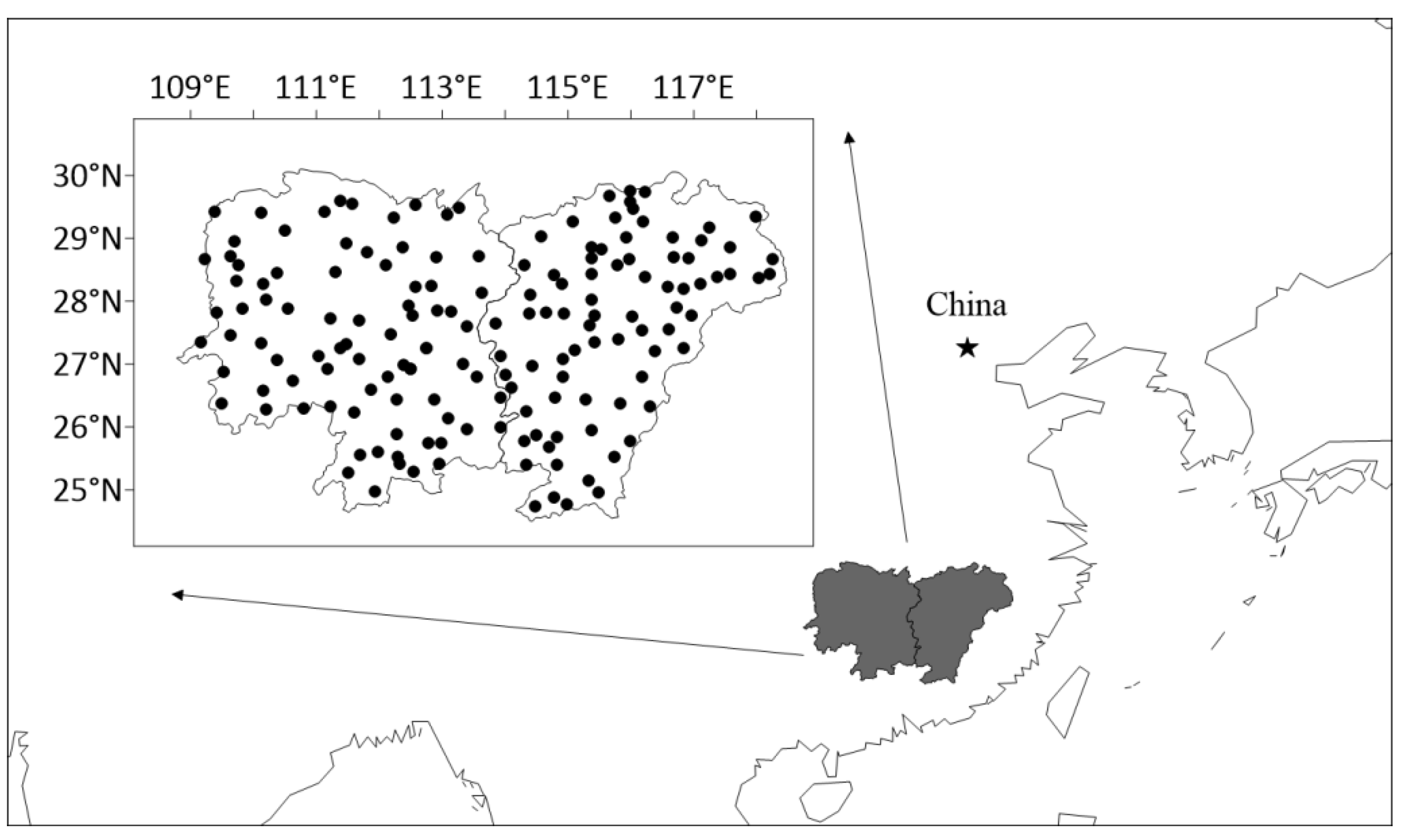
2.1. Data and Study Areas

Monthly precipitation data from 1961 to 2020 were obtained from 161 meteorological observation stations, provided by the National Meteorological Information Center of China Meteorological Administration. These data have been quality controlled and are widely used in climate prediction and analysis in China [35,36]. According to the National Standard of China (No. GB/T 20481-2017) and previous research [37,38], the standardized precipitation index (SPI) is calculated by obtaining the $\mathsf{\Gamma }$ distribution probability of precipitation in a certain period, taking normal standardization, and using the standardized cumulative frequency distribution of precipitation to divide the drought level. The probability density function of precipitation x in a certain period is as follows:

$$\mathrm{f}(x)=\frac{1}{{\beta }^r\mathsf{\Gamma }\left(r\right)}{x}^{r-t}{x}^{-x/\beta },$$

(1)

where the shape parameter $\beta$ and scale parameter $r$ are expressed as

$$\begin{array}{l}\widehat{r}=\frac{1+\sqrt{1+4A/3}}{4A}\\ \widehat{\beta }=\overline{x}/\widehat{r}\end{array}$$

(2)

where $A=\lg \overline{x}-\frac{1}{n}{\displaystyle \sum _{i=1}^n\lg x_i}$, $x_i$ is precipitation, and $\overline{x}$ is its climate average.

For the precipitation sample $x_0$, the probability ($F$) of sample $x$ being less than $x_0$ is calculated as follows:

$$\begin{array}{l}F(x<x_0)=\frac{1}{\sqrt{2\pi }}{\displaystyle {\int }_0^{x_0}{e}^{-Z^2/2}}dx\\ \mathrm{Z}=\mathrm{S}t-\frac{S[(c_{2}t+c_1)t+c_0]}{\left[(d_{3}t+d_2)t+d_1\right]t+1.0}\end{array}$$

(3)

where $\mathrm{t}=\sqrt{\ln \frac{1}{F^2}}$, and $F>0.5$, $F=1.0-F$, $S=1$, $F\le 0.5$, and $S=-1$, with parameters c₀ = 2.515517, c₁ = 0.802853, c₂ = 0.010328, d₁ = 1.432788, d₂ = 0.189269, and d₃ = 0.001308. The Z value obtained by Equation (3) is SPI. The calculation program can be downloaded from the following website: https://drought.unl.edu/monitoring/SPI/SPIProgram.aspx (accessed on 15 October 2022).

Then, we obtain SPI data for 1 month, 3 months, 6 months, 12 months, and 24 months. This study adopted the annual SPI (12 months) to explore the DWT and the related EWSs in the two-lake region. The two-lake region (study area) is situated in the middle reaches of the Yangtze River. The climatic characteristics of the two-lake basin can be summarized as follows. The climate is mild with four distinct seasons. There is sufficient heat and concentrated precipitation. The spring temperature is changeable, and the summer and autumn are dry. The cold period is short, and the hot period is long. In recent years, frequent floods and droughts have threatened the local ecological environment and agricultural production. The study area and 161 stations are marked in Figure 1.

2.2. Methods

2.2.1. Variance and Auto-Correlation Coefficient

Variance quantifies the deviation degree of the data in the sample from their mean $\overline{x}$, while the auto-correlation coefficient describes the degree of similarity between a given time series and a lagged version of itself over successive time intervals. In this study, the moving variance and auto-correlation coefficient of the sequence are adopted to investigate the EWSs for the DWT with respect to the SPI sequence. The detailed operations are as follows (Figure 2).

(a) Calculation of moving variance. Take the SPI sequence as an example. The total length of the SPI sequence is set to $L$, and a subsequence is selected from the sequence, which is called a sliding window and represented by ML. Then, another subsequence of the same length as ML is obtained by sliding, and this sliding length is called the sliding step, represented by MT. After the ML and MT are determined, multiple sub-sequences $L1$, $L2$, $L3$…… and $Ln$ with the same length are obtained by the sliding window method, and their variances are further calculated, thus obtaining a variance sequence $S1$, $S2$, $S3$…… and $S\mathrm{n}$. In this study, when calculating the variance, the ML is set to 120 months (10 years), and the MT is set to 3 months for the sliding window.

(b) Calculation of moving auto−correlation coefficient. Take the same SPI sequence as an example. By sliding the subsequence $L1$, $L2$, $L3$…… and $Ln$ forward by one lag time (LT), a new subsequence $L12$, $L22$, $L32$…… and $Ln2$ is obtained. Afterwards, by calculating the correlation coefficients of $L1$ and $L12$, $L2$ and $L22$, $L3$ and $L32$, …… and $Ln$ and $Ln2$, respectively, a sequence of correlation coefficients $\alpha 1$, $\alpha 2$, $\alpha 3$…… and $\alpha \mathrm{n}$ is obtained. Since the subsequences for calculating the correlation coefficient are all derived from the SPI sequence, the correlation coefficient here is thus called the auto-correlation coefficient. In this study, when calculating the auto-correlation coefficient by the sliding window, the ML is set to 120 months (10 years), the MT is set to 3 months, and the LT is set to 1 month.

2.2.2. Relationship between the CSD and the Increases in Auto-Correlations and Variances

When a stochastically forced system approaches a bifurcation at a threshold value of a control parameter, the CSD often results in an increase in both the auto-correlation coefficient and variance of the fluctuations [14,21]. An auto-regressive model is used to describe the periodic disturbance of the state variable as follows:

$$x_{n+1}=e^{\lambda \Delta t}{x}_n+s{\epsilon }_n,$$

(4)

where $x_n$ is the deviation of the state variable $x$ from the equilibrium state. The Δt represents the recovery period of the disturbance, and the $\lambda$ represents the recovery speed. $s$ and ${\epsilon }_n$ represent the standard deviation and white noise conforming to normal distribution, respectively.

When $\mathsf{\lambda }$ and $\mathsf{\Delta }\mathrm{t}$ are independent of $x_n$, this disturbance process can be written as a first−order auto−regressive model, AR(1):

$$x_{n+1}=\alpha x_n+s{\epsilon }_n,$$

(5)

where $\alpha =e^{\lambda \Delta t}$ represents the auto−correlation coefficient. It is 0 for white noise and is close to 1 for red noise.

For AR (1), it is calculated as follows:

$$Var(x_{n+1})=E(x_n^2)+{(E(x_n))}^2=\frac{s^2}{1-{\alpha }^2}.$$

(6)

The parameter $s$ represents the variance. Slowing down phenomenon occurs when the system approaches the critical point, and the recovery rate becomes slower and slower when it transits from small amplitude disturbance to equilibrium [39,40]. During the period of slowing down phenomenon, parameter $\lambda$ is close to 0, and the auto-correlation $\alpha$ approaches 1. Meanwhile, the variance tends toward infinity (Equation (6)). Therefore, when the system approaches the critical point, the increase in variance and auto-correlation coefficient can be considered as early warning signals. The variance and auto-correlation coefficient are studied to find the EWS for the complex dynamic system approaching the critical point.

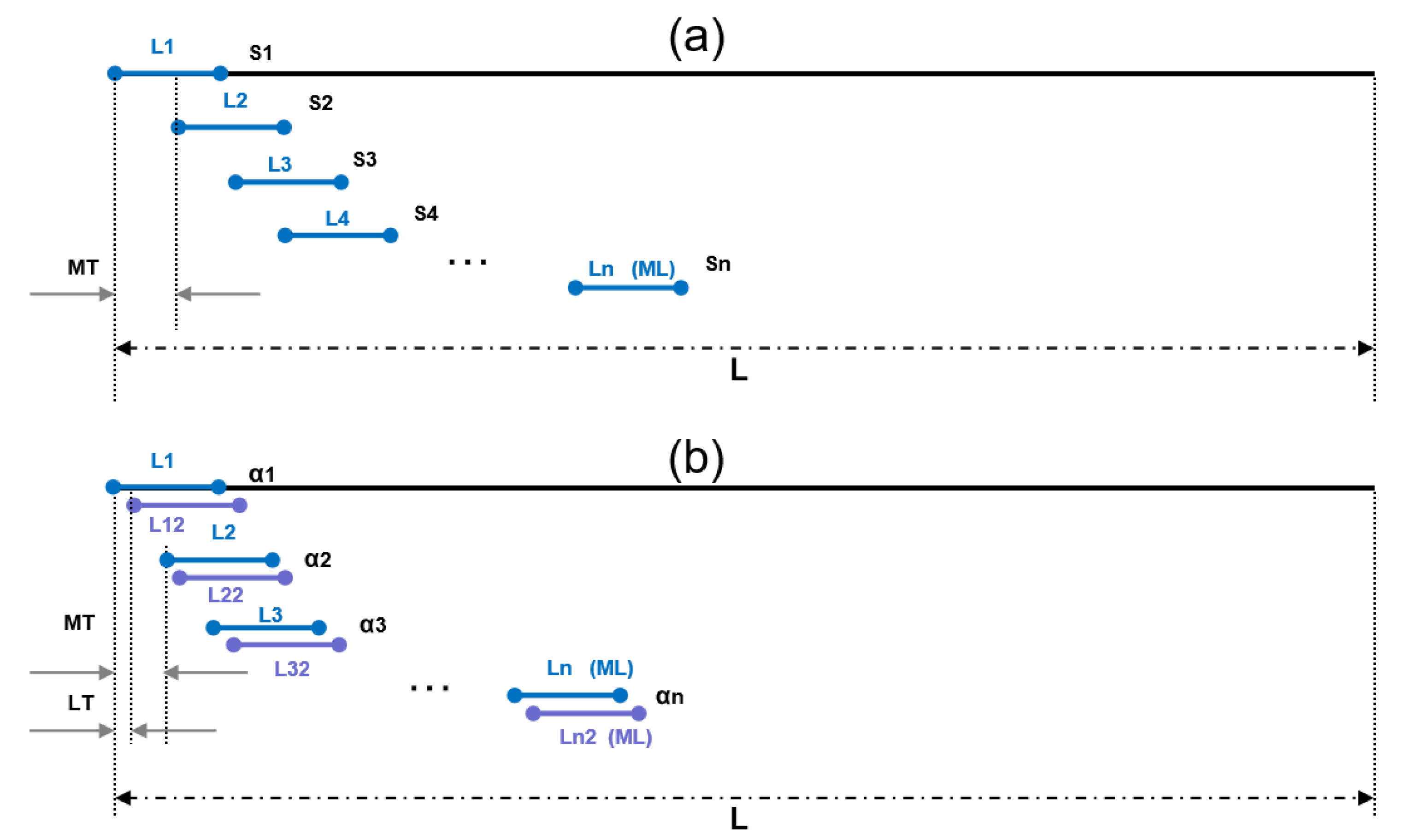
2.2.3. Moving t-Test Method

The MTT method is proposed to check the abrupt change in time sequence by testing the significant difference between the mean values of two samples. If the difference between the mean values of two subsequences exceeds a certain significance level, it can be considered that the mean value changed abruptly. For the time series $x$ with $n$ samples, a certain time is artificially set as the reference point, and the samples of the two sub-sequences $x_1$ and $x_2$ before and after the reference point are $n_1$ and $n_2$, respectively. The mean values of the two sub−sequences are $\overline{x_1}$ and $\overline{x_2}$, and the variances are $s_1^2$ and $s_2^2$, respectively. The defined statistics are

$$t=\frac{\overline{x_1}-\overline{x_2}}{s\cdot \sqrt{\frac{1}{n_1}+\frac{1}{n_2}}}.$$

(7)

$$s=\sqrt{\frac{n_1{s}_1^2+n_2{s}_2^2}{n_1+n_2-2}}.$$

(8)

Equation (7) follows the t-distribution with degree of freedom $\nu =n_1+n_2-2$. It should be noted that the selection of the subsequence for the MTT method is artificial. In this study, the subsequence length is changed repeatedly to detect the DWT time in the SPI sequence in different sub-regions.

3. Results and Analysis

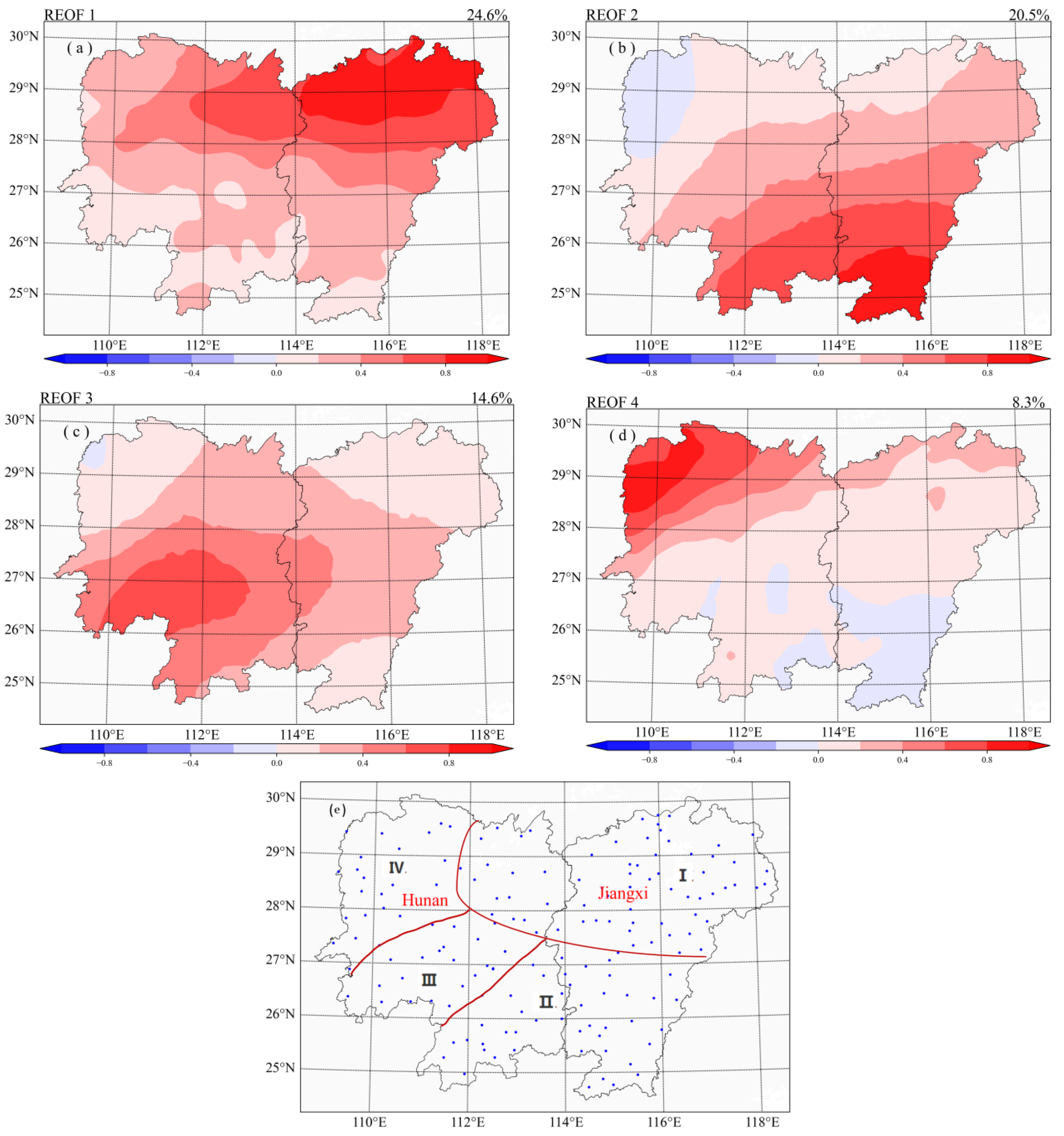
3.1. Regional Division Based on the REOF Method

The REOF method was proposed to study the spatial distribution difference in variables. The REOF method can increase the clarity of the feature field space and the stability of time, which is conducive to the extraction of the local features of the spatial distribution of climate elements. A detailed description about the REOF analysis method can be found in [41]. In this study, the REOF analysis method was firstly conducted on the sequence of SPI in the two-lake region in the study period, and 16 modes were obtained. Due to the complex topography of the two-lake region, the large spatio-temporal variation of the SPI-based drought index, and the complicated sub-regional characteristics of the drought, the variance contribution rate was rather low for each REOF mode. The cumulative variance contribution rate of the leading 16 REOF modes reached 88.88%, indicating that the convergence speed of eigenvalues was rather slow (

Table 1. Variance contribution rate and cumulative variance contribution rate of each REOF mode.

REOF Mode	1	2	3	4	5	6	7	8
Variance/%	24.59	20.47	14.64	8.25	6.00	2.27	1.94	1.46
Cumulative/%	24.59	45.05	59.70	67.95	73.95	76.22	78.16	79.62
REOF Mode	9	10	11	12	13	14	15	16
Variance/%	1.33	1.33	1.29	1.17	1.16	1.08	1.04	0.86
Cumulative/%	80.95	82.29	83.58	84.75	85.91	86.99	88.03	88.88

).

Figure 2 demonstrates the distributions of the leading four REOF modes of the SPI in the two-lake region during the past 60 years, which were obtained with the interpolation of station points. On a certain load vector field, the area where the absolute value of the load was ≥$0.5$ and was geographically connected is identified as an area with similar changes. This operation as applied to the leading four REOF modes (Figure 3a–d), and roughly four sub-regions can be obtained (Figure 3e). The cumulative variance contribution rate of the leading four REOF modes reached 67.95%, where the first three modes were the main contributing modes with the cumulative variance contribution rate being 59.7%, and the contribution rates were all below 10% in the other modes. Therefore, the leading four modes were selected for this study. Specifically, the stations with an absolute value for the load of ≥$0.5$ in the leading four modes were selected. Then, the grid area-weighted average method [42] was used to calculate the total SPI for each sub-region based on the SPI at each selected station. Finally, the DWT and related EWSs in the two-lake region were investigated based on the total SPI of each sub-region.

3.2. Characteristics of the DWT in Different Sub-Regions of the Two-Lake Region

Figure 3 shows the variation characteristics of the SPI sequence and the detection of the dry-to-wet or wet-to-dry events in sub-region I of the two-lake region. Figure 3a reveals that the SPI sequence in sub-region I presents the obvious interannual and interdecadal variation characteristics. In addition, the filtered sequence displays that there are relatively obvious dry-to-wet events in 1990 and 2012, with an obvious wet-to-dry event in 2003. All these events are collectively referred to as DWT events (abrupt changes). The research showed that the dry and wet status in the two-lake basin has obvious interdecadal variations [4,5]. In particular, the dry-to-wet event around 1990 has caused wide concern. Figure 3b,c reveal the abrupt changes in the SPI sequence in sub-region I detected by the MTT method. When the sliding window’s width $t$ was set to 10 years, multiple DWT events can be found in the SPI sequence, which were especially obvious in 1975, 1992, and 2003 (all passed the significance test at the significance level of 0.01). When the sliding window width was set to 15 years, two obvious DWT events in 1990 and 2003 can also be found. Combined with the interdecadal variations of the SPI sequence (Figure 4a), it can be inferred that there are two obvious DWT (critical transitions) in the SPI sequence in 1990 and 2003 in sub-region I based on the MTT method. Similar operations were conducted on the SPI sequence in sub-regions II, III, and IV (figures omitted), and the DWT time for each sub-region was obtained (

Table 2. Dry–wet state conversion time in different sub−regions.

Sub−Region	I	II	III	IV
Dry–wet State conversion time	1990/2003	1993/2003	1991/2004	1994/2004

). Generally, there were obvious DWT events in the four sub-regions of the two-lake region in the early 1990s and early 2000s. Wu et al. [43] analyzed the circulation background of the DWT events in the Dongting Lake basin with respect to 500 hPa geopotential height and 200 hPa zonal wind. The results showed that the circulation backgrounds in 1961–1992 and 2003–2020 were favorable for less precipitation and thus caused the drought in the Dongting Lake basin, while the circulation background in 1993–2002 led to more precipitation and even floods in the Dongting Lake basin. Since the same operation is also applicable to the two-lake region, it will not be covered here. This is a rational analysis of the two DWT events focusing on the circulation background.

3.3. Early Warning Signals for DWT Events in Different Sub-Regions of the Two-Lake Region

In this section, the EWSs are explored for the DWT events in the two-lake region by the variance and auto-correlation coefficient that characterize the CSD phenomenon.

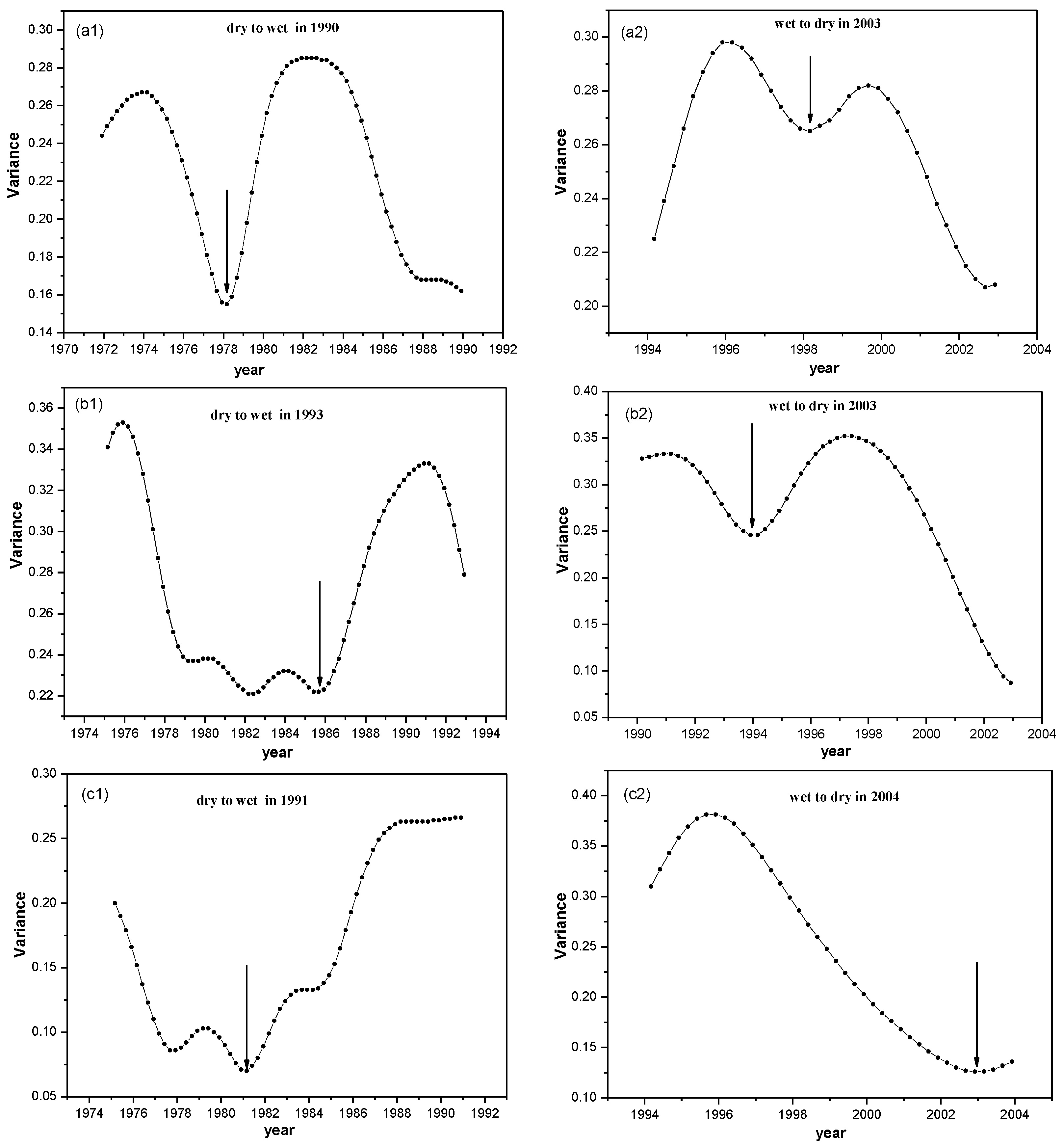
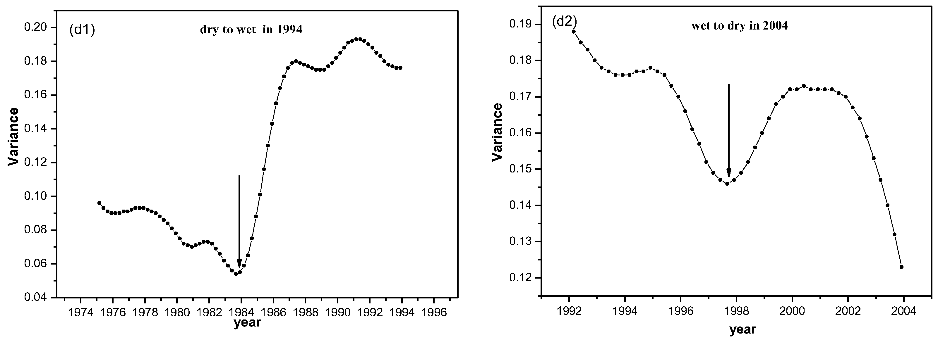
3.3.1. Early Warning Signals Based on the Variance

In this section, according to the detected time when the DWT events occurred in each sub-region, the EWSs for the DWT events are investigated by using the variance that characterizes the CSD phenomenon.

Figure 5(a1–d2) shows the variance signal-based detection of the DWT in the SPI sequence in different sub-regions of the two-lake region. Detailed operations are displayed in Figure 2. Figure 5(a1–a2) shows the variance signal-based detection of the DWT in the SPI sequence in sub-region I. The variance has increased since around 1978 (marked by the arrow in Figure 5(a1)). According to the CSD theory, the CSD phenomenon of increasing variance and auto-correlation detected when the complex nonlinear system approaches the critical point that can be used as an EWS for the DWT. That is, the increase in variance since 1978 indicated a dry-to-wet event in the future (1990). Therefore, it is concluded that the variance-based early warning signal appeared 12 years earlier than the occurrence of this SPI-based dry-to-wet event, suggesting that the variance is a good indicator for the prediction of the DWT. In addition, the increase in variance since around 1998 (marked by the arrow in Figure 5(a2)) also indicated a wet-to-dry event in the future (2003). Similar operations were also conducted in other sub-regions, and the EWSs of the increase in variance were about 10 years ahead of the DWT events, which can be found in all the sub-regions (Figure 5(b1–d2)). It is worth noting that, in some sub-regions (such as sub-region II, Figure 5(b1)), there were several staged increases (around 1982 and around 1986) in the variance before the DWT event. This is attributed to the fact that different settings of ML and MT have a certain influence on the stability of the detection results. Previous studies showed that for a certain amount of data, the larger the ML and the longer the MT were, the more stable the result was [24,25,26,27]. That is, the larger the ML and the longer the MT were, the more reliable the detected signal was. By changing the ML and MT, the variance signal in 1986 always exists. Hence, the early warning signal for the SPI-based DWT event in 1993 in sub-region II appeared in 1986. In summary, although the DWT time varies in the different sub-regions, the variance signal-based detection in all the sub-regions in the two-lake region shows that there is a CSD phenomenon, with a variance increase 10 years ahead of the DWT event. This confirms the validity of the variance signal, which is indicative of the occurrence of the DWT events.

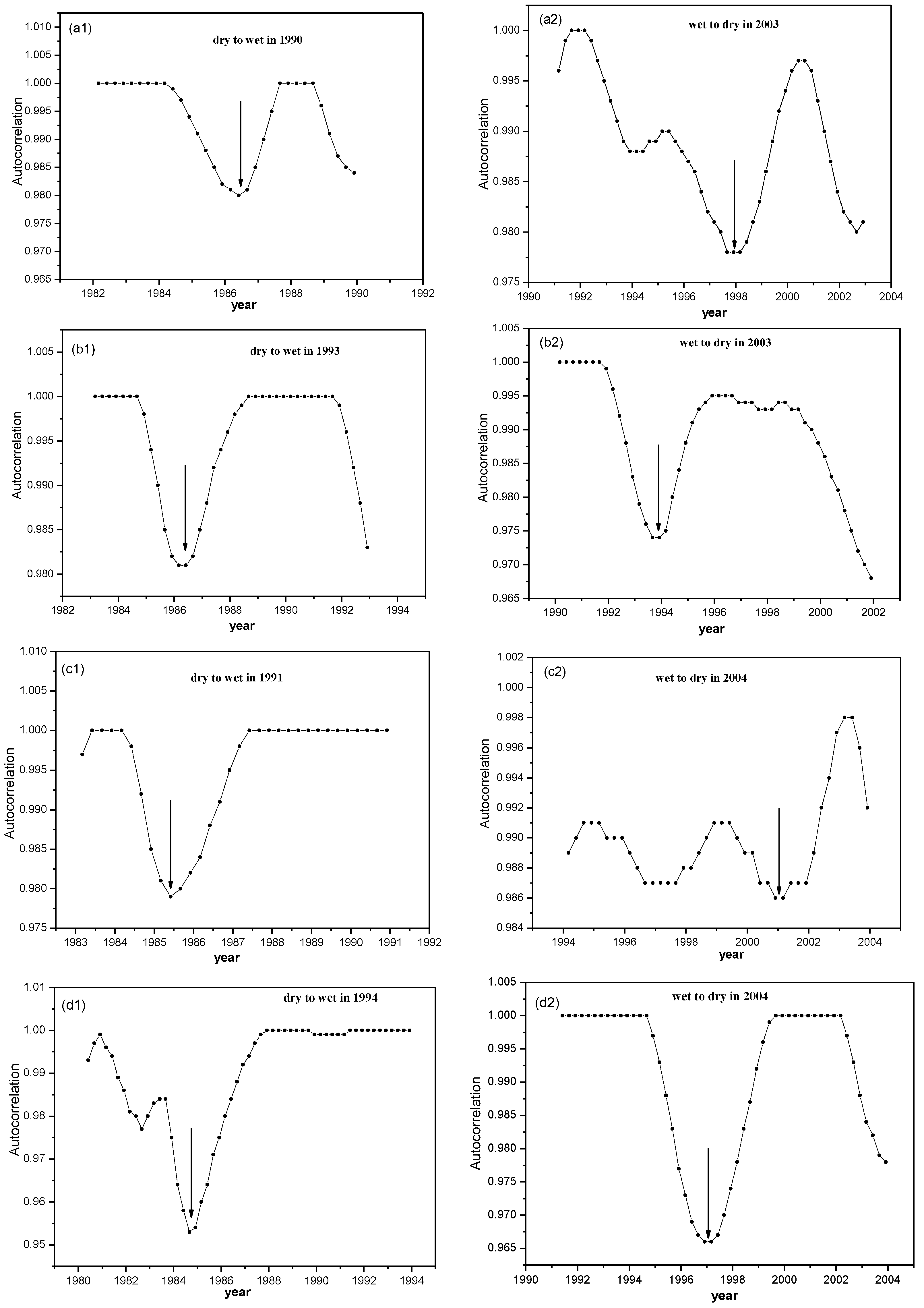
3.3.2. Early Warning Signals Based on the Auto-Correlation Coefficient

The CSD theory showed that the auto-correlation coefficient increases as the nonlinear system approaches the critical point. In this section, the early warning signals (EWSs) for the DWT are investigated by using the auto-correlation coefficient that characterizes the CSD phenomenon.

Figure 6(a1–d2) shows the auto-correlation coefficient signal-based detection of the DWT in the SPI sequence at representative stations in different sub-regions. Figure 6(a1–a2) shows the auto-correlation coefficient signal-based detection of the DWT in sub-region I of the two-lake region. Figure 6(a1) displays that the auto-correlation coefficient has increased since around 1986 (marked by the arrow). As the CSD resulted in a decrease in the internal change rate of the dry-wet state, and as the status of the complex nonlinear system at any time became more and more similar to its previous status, the auto-correlation coefficient of the SPI sequence approached 1; that is, the early warning signal for the dry-to-wet event in 1990 appeared around 1986. Hence, the early warning signal of the increasing auto-correlation coefficient appeared four years before the dry-to-wet event in sub-region I of the two-lake region, which is a good indicator for the prediction of the DWT in the two-lake region. Similarly, the increase in the auto-correlation coefficient since around 1998 (marked by the arrow in Figure 6(a2)) also indicated a wet-to-dry event in the future (2003). Similar operations conducted on other sub-regions revealed that the EWSs of the increase in the auto-correlation coefficient were about 10 years ahead of the DWT events, which can be detected in all sub-regions (Figure 6(b1–d2)). Note that there were also false signals in the auto-correlation coefficient-based signals (for example, as shown in Figure 6(c2)), which can be discriminated by using the CSD phenomenon mentioned in the previous section, i.e., under the condition of a certain amount of data, the larger the ML and the longer the MT were, the more stable the results were.

In summary, the occurrence time of the EWSs for the SPI-based DWT events detected by the variance were basically consistent with that detected by the auto-correlation coefficient, with the performance of the auto-correlation coefficient-based signal being slightly better. This further confirmed the feasibility of studying the EWSs for the DWT events in different sub-regions of the two-lake region based on the CSD theory.

4. Conclusions and Discussions

The DWT is a typical abnormal precipitation event. Against the background of global warming, the DWT events in the two-lake region have become increasingly frequent, which often lead to regional floods or droughts. If efficient early warnings can be released ahead of the DWTs, the government and relevant departments would have enough time to plan and take effective measures to minimize disaster losses as much as possible. Therefore, there is important theoretical and practical significance to conduct research on the prediction of and early warnings for DWT events in the two-lake region. Considering the complex nonlinear characteristics of the DWT, nonlinear science-related theories and methodologies were applied in this study. Firstly, the REOF method was used to divide the two-lake region into four sub-regions with respect to the SPI. Then, the MTT method was applied to the sequence of SPI data from the four sub-regions of the two-lake region in the past 60 years, aiming to detect the occurrence time of DWT events. Finally, based on the principle of CSD, the EWSs for the SPI-based DWT events in the four sub-regions of the two-lake region were discussed, and the main conclusions are as follows.

(1)

Based on the REOF method, the two-lake region can be divided into four climate zones, and the cumulative variance contribution rate of the four leading modes reaches 67.95%, which meets the REOF zoning requirements.

(2)

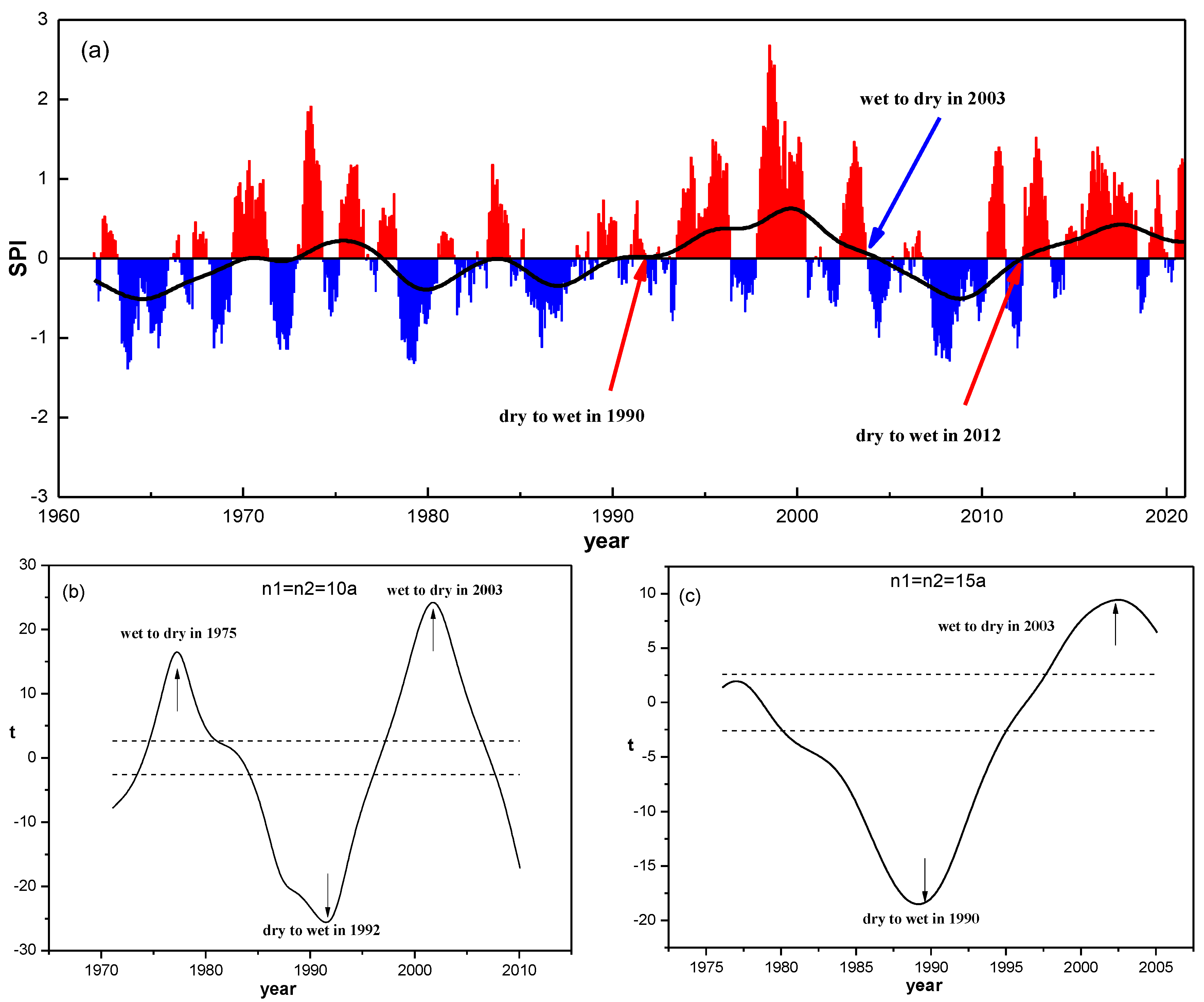
Detections of the SPI sequence from the four sub-regions reveal that there were obvious DWT events in each sub-region, with the emphasis in this study placed on the two most obvious DWT events that occurred in each sub-region in the early 1990s and early 2000s.

(3)

The featured CSD phenomenon, by varying degrees of increase in the variance and auto-correlation coefficient, appeared about 10 years before the SPI-based DWT events in all four sub-regions, which demonstrates the feasibility of exploring the EWSs for DWT events using the CSD theory.

Based on the research on the DWT and corresponding EWSs in the two-lake region, the feasibility of taking the two physical quantities (variance and auto-correlation coefficient) that characterize the CSD phenomenon as EWSs for detecting abrupt changes in climate data was verified. In addition, the introduction of the CSD theory was of great significance for an in-depth understanding of the SPI-based DWT events and for detecting the related EWSs. As a method with a wide application prospect, it is hoped that this method can provide important reference basis for the prediction of drought and flood as well as disaster prevention and mitigation in the Yangtze River basin. Note that the research based on the SPI revealed that the increase in the auto-correlation coefficient and variance caused by the CSD phenomenon may dynamically act as the EWSs before the DWT events. However, other issues such as the characteristics of the circulations and external forcing changes before and after the DWT and the relationships of the CSD phenomenon with the amplitude and intensity of the abrupt changes in the DWT events need further investigation.

It is worth noting that climate change often has a significant impact on human society, economic development, and agriculture [44]. Studying the EWSs of climate change can remind people to prepare for disasters. Kelman et al. [45] pointed out that the location, time, and audience may determine the impact of a climate change disaster. The DWT we have studied in this manuscript has had a serious impact on agriculture in the two-lake region for a long time. The EWSs given in the conclusion can help people to cope with DWT disasters.

References

1. Huang, Q.; Sun, Z.; Opp, C.; Lotz, T.; Jiang, J.; Lai, X. Hydrological Drought at Dongting Lake: Its Detection, Characterization, and Challenges Associated With Three Gorges Dam in Central Yangtze, China. Water Resour. Manag. Int. J. 2014, 28, 5377–5388. [Google Scholar] [CrossRef]
2. Grubler, A. IPCC Fifth Assessment Report. Weather 2014, 68, 310. [Google Scholar]
3. Tang, G.; Ding, Y.; Wang, S.; Ren, G.; Liu, H.; Zhang, L. Comparative analysis of the time series of surface air temperature over China for the last 100 years. Adv. Clim. Chang. Res. 2010, 1, 11–19. [Google Scholar] [CrossRef]
4. Zhang, J.; Liao, Y.; Wu, H.; Zhang, J.; Zhao, H. Characteristics of Atmospheric Circulation Anomalies and Drought in Summer and Autumn in Hunan Province. J. Arid Meteorol. 2018, 36, 353–364. (In Chinese) [Google Scholar]
5. Wu, H.; Zhang, J.; Yan, P.; Zeng, Y.; Duan, L. The Research on Drought Characteristics of SPI at Different Time Scales in Hunan Province. Adv. Meteorol. Sci. Technol. 2021, 11, 139–147. (In Chinese) [Google Scholar]
6. Yang, S.; Wu, B.; Zhang, R.; Zhou, S. Relationship between an abrupt drought-flood transition over mid-low reaches of the Yangtze River in 2011 and the intraseasonal oscillation over mid-high latitudes of East Asia. Acta Meteorol. Sin. 2013, 27, 129–143. [Google Scholar] [CrossRef]
7. Wu, Z.; Li, J.; He, J.; Jiang, Z. Large-scale atmospheric singularities and summer long-cycle droughts-floods abrupt alternation in the middle and lower reaches of the Yangtze River. Chin. Sci. Bull. 2006, 16, 2027–2034. [Google Scholar] [CrossRef]
8. Li, X.; Ye, X. Spatiotemporal characteristics of dry-wet abrupt transition based on precipitation in Poyang Lake Basin, China. Water 2015, 5, 1943–1958. [Google Scholar] [CrossRef] [Green Version]
9. Li, W.; Fu, R. Transition of the Large-Scale Atmospheric and Land Surface Conditions from the Dry to the Wet Season over Amazonia as Diagnosed by the ECMWF Re-Analysis. Am. Meteorol. Soc. 2004, 13, 2637–2651. [Google Scholar] [CrossRef]
10. Espinoza, J.; Arias, P.; Moron, V.; Junquas, C.; Segura, H.; Sierra-Pérez, J.; Wongchuig, S.; Condom, T. Recent changes in the atmospheric circulation patterns during the dry-to-wet transition season in south tropical South America (1979–2020): Impacts on precipitation and fire season. J. Clim. 2021, 22, 9025–9042. [Google Scholar] [CrossRef]
11. Ding, R.; Li, J. Relationships between the Limit of Predictability and Initial Error in the Uncoupled and Coupled Lorenz Models. Adv. Atmos. Sci. 2012, 29, 1078–1088. [Google Scholar] [CrossRef]
12. Wan, S.; Feng, G.; Dong, W.; Li, J.; Gao, X.; He, W. On the Climate Prediction of Nonlinear and Non-stationary Time Series with the EMD Method. Chin. Phys. B 2005, 14, 628–633. [Google Scholar]
13. Ding, R.; Liu, B.; Gu, B.; Li, J.; Li, X. Predictability of Ensemble Forecasting Estimated Using the Kullback-Leibler Divergence in the Lorenz Model. Adv. Atmos. Sci. 2019, 36, 837–846. [Google Scholar] [CrossRef]
14. Feng, G.-L.; Yang, J.; Zhi, R.; Zhao, J.-H.; Gong, Z.-Q.; Zheng, Z.-H.; Xiong, K.-G.; Qiao, S.-B.; Yan, Z.; Wu, Y.-P.; et al. Improved prediction model for flood-season rainfall based on a nonlinear dynamics-statistic combined method. Chaos Solitons Fractals 2020, 140, 110160. [Google Scholar] [CrossRef]
15. Fan, M.; Jiang, J. Study of Heavy Causes Contrasting 1999 to 1998 Summer over Changjiang River Basin. Meteorol. Mon. 2001, 27, 38–41. (In Chinese) [Google Scholar]
16. Gao, H.; Wang, Y. Sea Surface Temperature and the General Circulation in 2007 and Their Influences on the Climate of China. Meteorol. Mon. 2008, 34, 107–112. (In Chinese) [Google Scholar]
17. Scheffer, M.; Bascompte, J.; Brock, A.; Brovkin, V.; Carpenter, S.; Dakos, V.; Held, H.; Nes, E.; Rietkerk, M.; Sugihara, G. Early-warning signals for critical transitions. Nature 2009, 461, 53–59. [Google Scholar] [CrossRef] [PubMed]
18. Fisher, L.; Scheffer, M. Critical Transitions in Nature and Society. Am. J. Psychol. 2011, 124, 365–367. [Google Scholar] [CrossRef] [Green Version]
19. Gopalakrishnan, E.; Sharma, Y.; John, T.; Dutta, P.; Sujith, R. Early warning signals for critical transitions in a thermoacoustic system. Sci. Rep. 2016, 6, 35310. [Google Scholar] [CrossRef] [Green Version]
20. Lenton, T.; Livina, V.; Dakos, V.; Nes, E.; Scheffer, M. Early warning of climate tipping points from critical slowing down: Comparing methods to improve robustness. Philos. Trans. R. Soc. A Math. Phys. Eng. Sci. 2012, 370, 1185–1204. [Google Scholar] [CrossRef]
21. Alley, R.; Marotzke, J.; Nordhaus, W.; Overpeck, J.; Peteet, D.; Pielke, R.; Pierrehumbert, R.; Rhines, P.; Stocker, T.; Talley, L. Abrupt Climate Change. Science 2003, 299, 2005–2010. [Google Scholar] [CrossRef] [PubMed] [Green Version]
22. He, W.; Xie, X.; Mei, Y.; Wan, S.; Zhao, S. Decreasing predictability as a precursor indicator for abrupt climate change. Clim. Dyn. 2021, 56, 3899–3908. [Google Scholar] [CrossRef]
23. Carpenter, S.; Brook, W. Rising variance: A leading indicator of ecological transition. Ecol. Lett. 2006, 9, 311–318. [Google Scholar] [CrossRef] [PubMed]
24. Guttal, V.; Jayaprakash, C. Changing skewness:An early warning signal of regime shifts in ecological systems. Ecol. Lett. 2008, 11, 450–460. [Google Scholar] [CrossRef] [PubMed] [Green Version]
25. Yu, L.; Hao, B. Phase Transitions and Critical Phenomena; Beijing Scientific Press: Beijing, China, 1984. (In Chinese) [Google Scholar]
26. Yan, R.; Jiang, C.; Zhang, L. Study on critical slowing down phenomenon of radon concentrations in water befer the Wenchuan Ms 8.0 earthquake. Chin. J. Geophys. 2011, 54, 1817–1826. (In Chinese) [Google Scholar]
27. Wu, H.; Feng, G.; Hou, W.; Yan, P. The early warning signals of abrupt climate change in different regions of china. Acta Phys. Sin. 2013, 62, 059202. (In Chinese) [Google Scholar] [CrossRef]
28. Wu, H.; Hou, W.; Yan, P. Using the principle of critical slowing down to discuss the abrupt climate change. Acta Phys. Sin. 2013, 62, 039206. (In Chinese) [Google Scholar] [CrossRef]
29. Wu, H.; Hou, W.; Yan, P.; Zhang, Z.; Wang, K. A study of the early warning signals of abrupt change in the Pacific decadal oscillation. Chin. Phys. B 2015, 24, 089201. [Google Scholar] [CrossRef]
30. Tong, J.L.; Wu, H.; Hou, W.; Wei, H.; Wen-Ping, H.; Jie, Z. The early warning signals of abrupt temperature change in different regions of China over recent 50 years. Chin. Phys. B 2014, 23, 049201. [Google Scholar] [CrossRef]
31. Yan, P.; Feng, G.; Hou, W. A novel method for analyzing the process of abrupt climate change. Nonlinear Process. Geophys. 2015, 22, 249–258. [Google Scholar] [CrossRef] [Green Version]
32. He, W.; Zhao, S.; Liu, Q.; Jiang, Y.; Deng, B. Long-range correlation in the drought and flood index from 1470 to 2000 in eastern China. Int. J. Climatol. 2016, 36, 1676–1685. [Google Scholar] [CrossRef]
33. He, W.; Liu, Q.; Gu, B.; Zhao, S. A novel method for detecting abrupt dynamic change based on the changing Hurst exponent of spatial images. Clim. Dyn. 2016, 47, 2561–2571. [Google Scholar] [CrossRef]
34. Xie, X.; He, W.; Gu, B.; Mei, Y. Can kurtosis be an early warning signal for abrupt climate change? Clim. Dyn. 2019, 52, 6863–6876. [Google Scholar] [CrossRef]
35. Zhao, T.B.; Ai, L.K.; Feng, J.M. An Intercomparison between NCEP Reanalysis and Observed Data over China. Clim. Environ. Res. 2004, 9, 278–294. [Google Scholar]
36. Zhang, S.Q.; Cao, S.S.; Hu, L.T.; Cai, C.l.; Tu, Y.; Lin, M. Spatio-temporal variation of atmospheric CH4 concentration and its driving factors in monsoon Asia. Chin. J. Appl. Ecol. 2021, 32, 1406–1416. [Google Scholar]
37. Mckee, T.; Doesken, N.; Kleist, J. The Relationship of Drought Frequency and Duration to Time Scales. In Proceedings of the 8th Conference on Applied Climatology, Hanover, Germany, 17–22 January 1993. [Google Scholar]
38. Belayneh, A.; Adamowski, J. Standard Precipitation Index Drought Forecasting Using Neural Networks, Wavelet Neural Networks, and Support Vector Regression. Appl. Comput. Intell. Soft Comput. 2014, 2012, 794061. [Google Scholar] [CrossRef] [Green Version]
39. Dakos, V.; Scheffer, M.; Nes, E.; Brovkin, V.; Petoukhov, V.; Held, H. Slowing down as an early warning signal for abrupt climate change. Proc. Natl. Acad. Sci. USA 2008, 105, 14308–14312. [Google Scholar] [CrossRef] [Green Version]
40. Held, H.; Kleinen, T. Detection of climate system bifurcations by degenerate fingerprinting. Geophys. Res. Lett. 2004, 31, L23207. [Google Scholar] [CrossRef] [Green Version]
41. Richman, M. Review article, rotation of principal components. J. Climatol. 1986, 6, 293–335. [Google Scholar] [CrossRef]
42. Jones, P.; Groisman, P.; Coughlan, M.; Plummer, N.; Wang, W.; Karl, T. Assessment of urbanization effects in time series of surface air temperature over land. Nature 1990, 347, 169–172. [Google Scholar] [CrossRef]
43. Wu, H.; Hou, W.; Zuo, D.; Yan, P.; Zeng, Y. Early-Warning Signals of Drought-Flood State Transition over the Dongting Lake Basin Based on the Critical Slowing Down Theory. Atmosphere 2021, 12, 1082. [Google Scholar] [CrossRef]
44. Kelman, I.; Glantz, M.H. Early Warning Systems Defined; Springer: Dordrecht, Germany, 2014. [Google Scholar]
45. Luca, D.; Versace, P. Diversity of rainfall thresholds for early warning of hydro-geological disasters. Adv. Geosci. 2017, 44, 53–56. [Google Scholar] [CrossRef]
Figure 1. The map of study area and locations of stations.
Atmosphere 14 00126 g001
Figure 2. (a) Calculation of the variance and (b) auto–correlation coefficient using the sliding window method.
Atmosphere 14 00126 g002
Figure 3. Leading four rotating load vector fields of the SPI sequence in the two-lake region during the last 60 years and corresponding regional division. (a) Region REOF1-I; (b) region REOF2-II; (c) region REOF3-III; (d) region REOF4-IV; (e) regional division map.
Atmosphere 14 00126 g003
Figure 4. Temporal variation of the SPI sequence in sub–region I of the two−lake region and detection of the DWT. (a) Variation of SPI sequence, where red bar represents positive SPI, blue bar represents negative SPI, and the black curve indicates the decadal trend in the filtered sequence. (b) DWT detection of the filtered SPI sequence with the sliding window width of n being 10 years. (c) DWT detection of filtered SPI sequence with the sliding window width of n being 15 years. In addition, the dashed lines in Figure 4b,c indicate the critical values at significance level of 0.01.
Atmosphere 14 00126 g004
Figure 5. Variance signal-based detection of DWT in different sub-regions of the two-lake region, where ML is set to 10 years, and MT is set to 3 months for the sliding window. (a1d2) correspond to four different sub-regions. The left and right figures correspond to the two DWT events in the early 1990s and early 2000s, respectively.
Atmosphere 14 00126 g005aAtmosphere 14 00126 g005b
Figure 6. Auto-correlation coefficient signal-based detection of DWT in different sub-regions of the two-lake region. The ML is set to 10 years, the MT is set to 3 months, and the LT is set to 1 month for the sliding window. (a1d2) correspond to the four sub-regions. The left and right figures correspond to the two DWT events in the early 1990s and early 2000s, respectively.
Atmosphere 14 00126 g006