
Aerobiological Monitoring in an Indoor Occupational Setting Using a Real-Time Bioaerosol Sampler
 and
and
Abstract
:1. Introduction
2. Materials and Methods
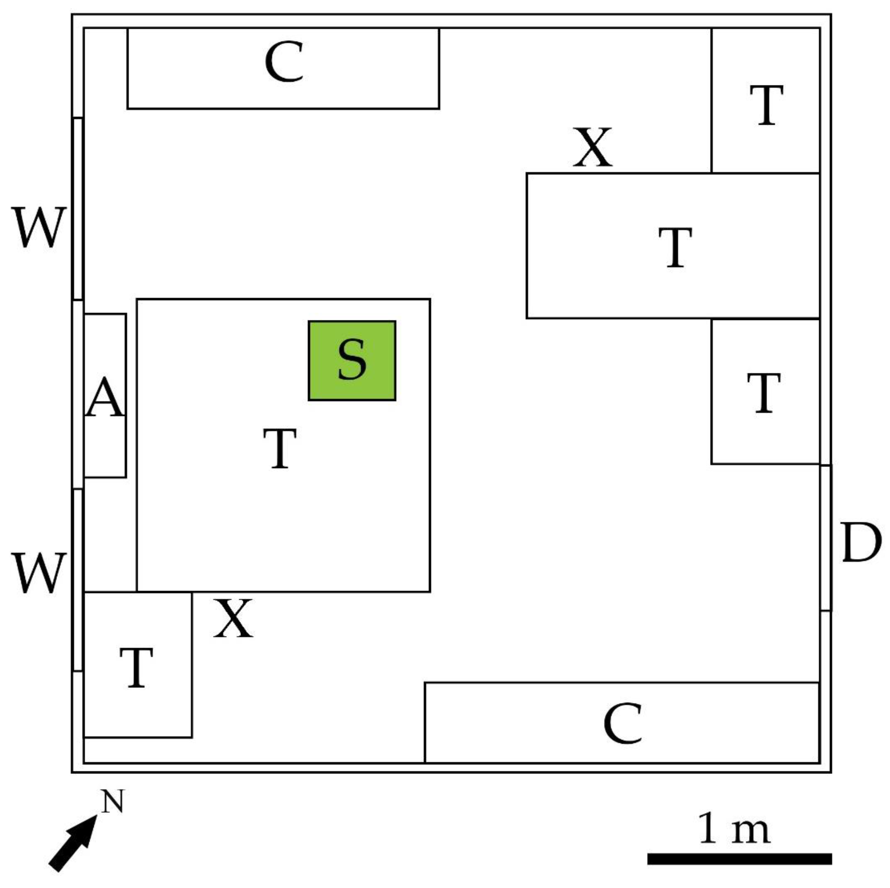
2.1. Study Area
2.2. Sampling Method and Particle Classification
- -
- A 635 nm diode laser used for particle sizing and shape detection;
- -
- A quadrant photomultiplier tube used to determine particle shape from forward scattered light;
- -
- A UV xenon lamp emitting light at a wavelength of 280 nm (Xe1);
- -
- A UV xenon lamp emitting light at a wavelength of 370 nm (Xe2);
- -
- A detector channel for particle fluorescence emission from 310–400 nm (FL1);
- -
- A detector channel for particle fluorescence emission from 420–650 nm, particle count and particle size (FL2).
- -
- The signal detected by the FL1 detector (310–400 nm) after the excitation at 280 nm was labeled as Channel A;
- -
- The signal detected by the FL2 detector (420–650 nm) after excitation at 280 nm was labeled as Channel B;
- -
- The signal detected by the FL2 detector after excitation at 370 nm was labeled as Channel C.
2.3. Data Analysis
- -
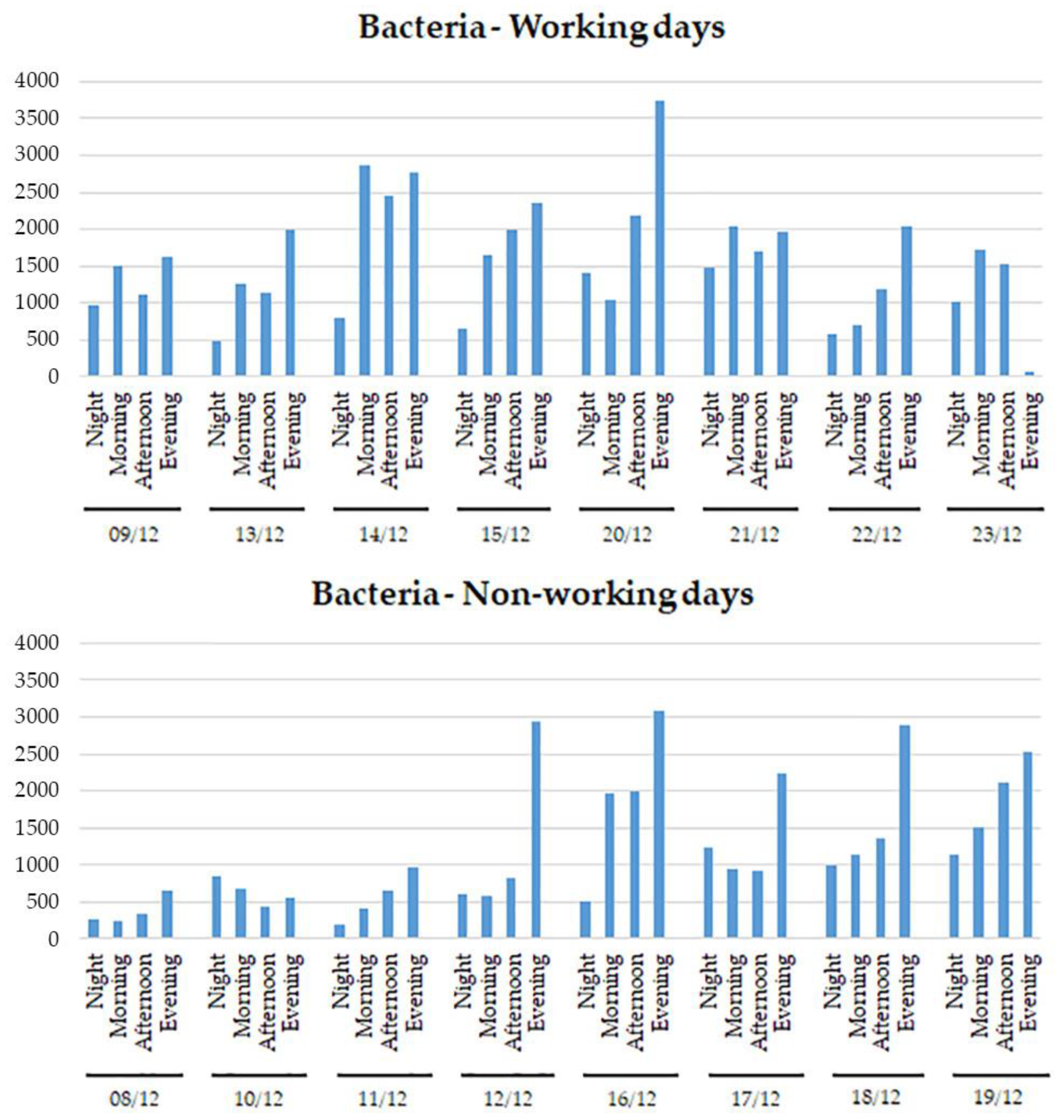
- Night: 0:00–5:59
- -
- Morning: 6:00–11:59
- -
- Afternoon: 12:00–17:59
- -
- Evening: 18:00–23:59
3. Results
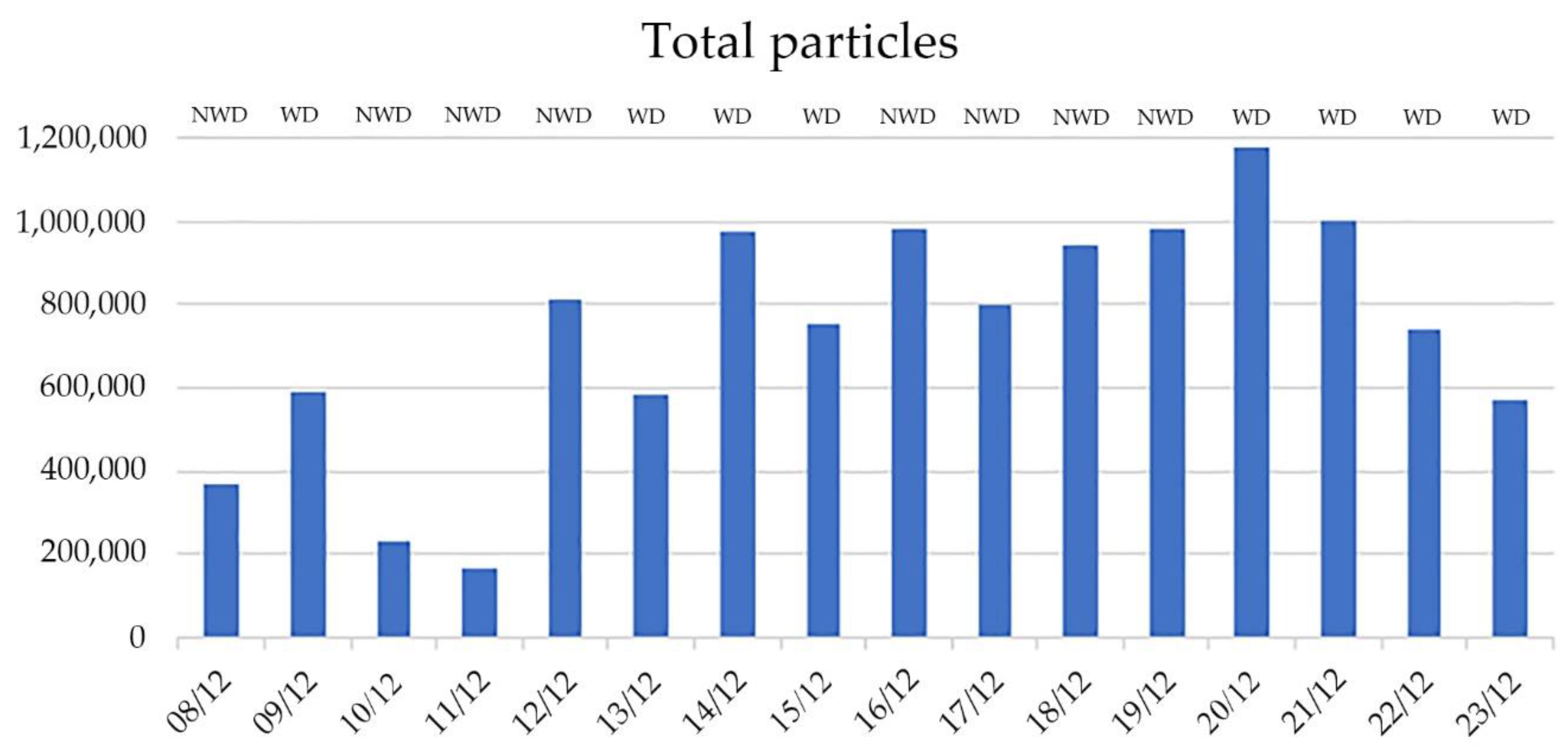
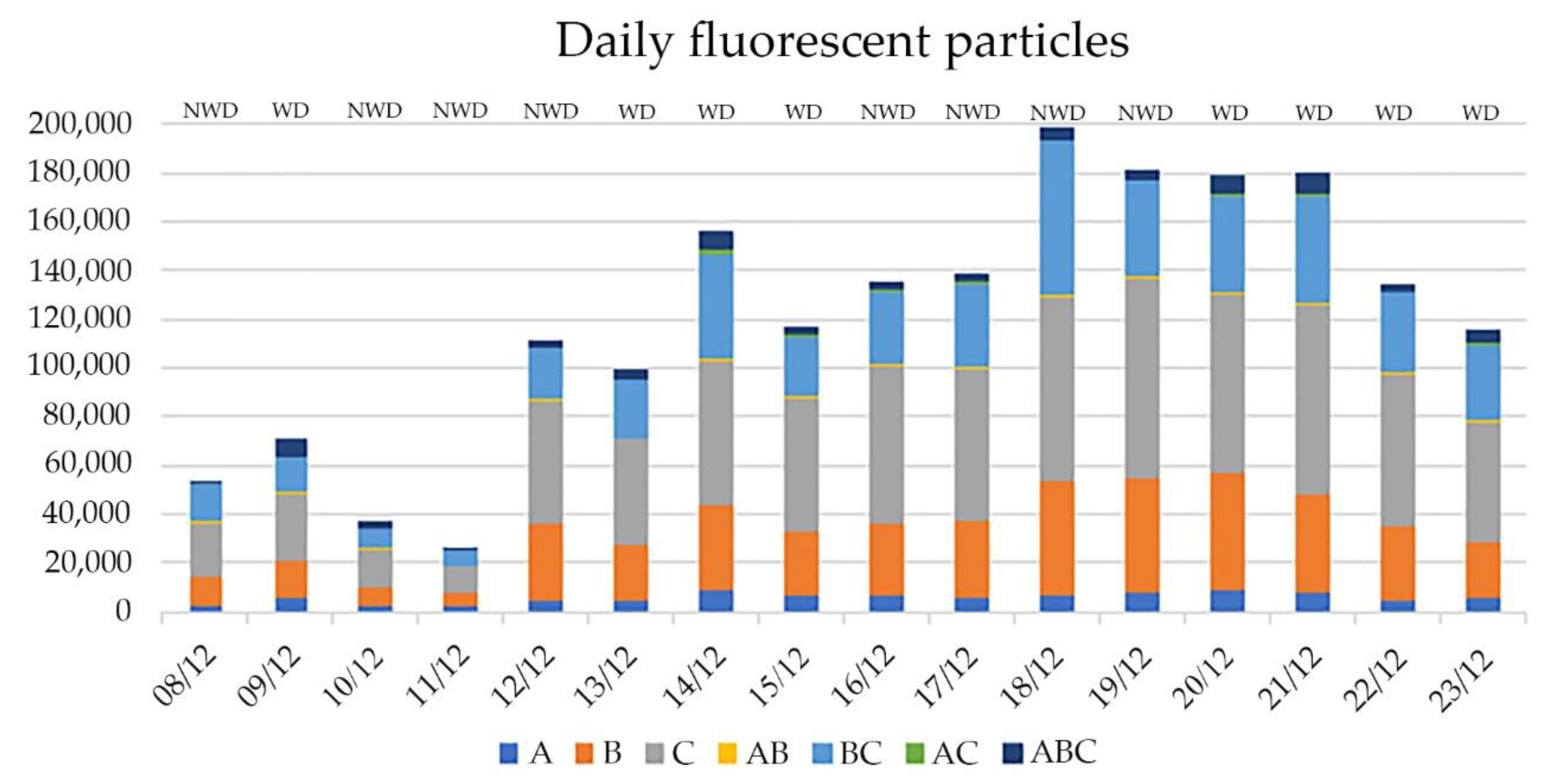
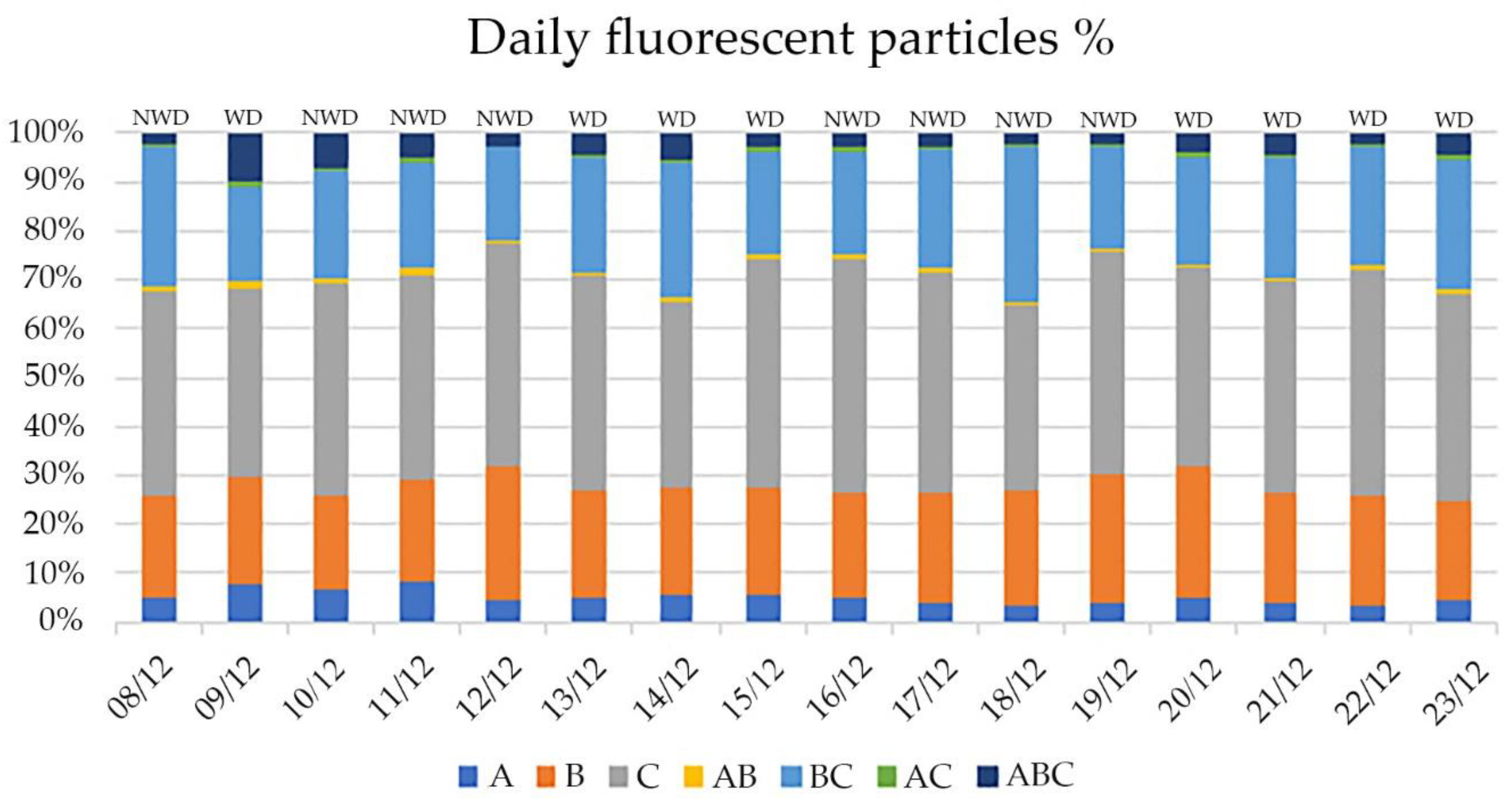
3.1. Total and Daily Distribution of Particles
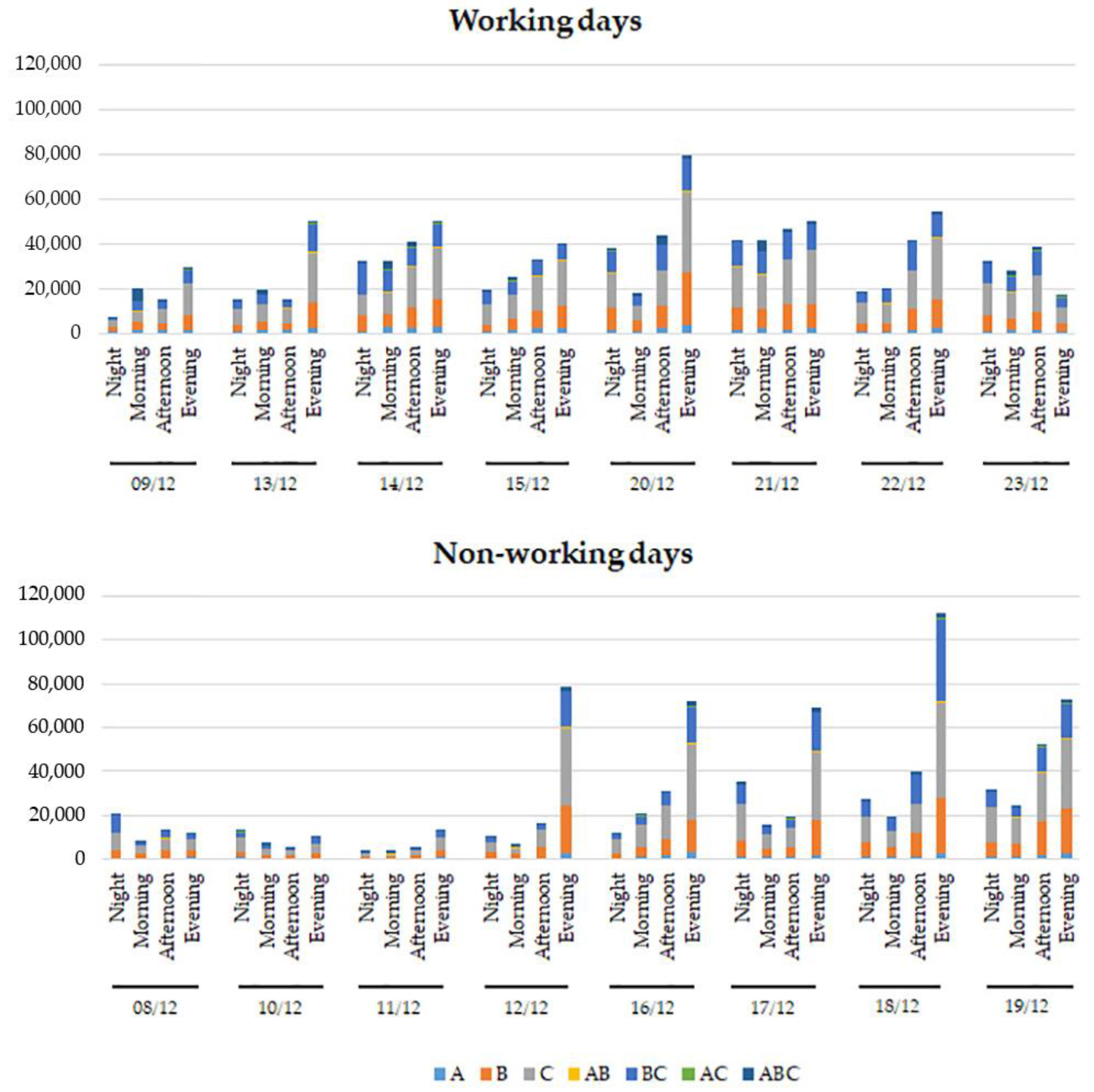
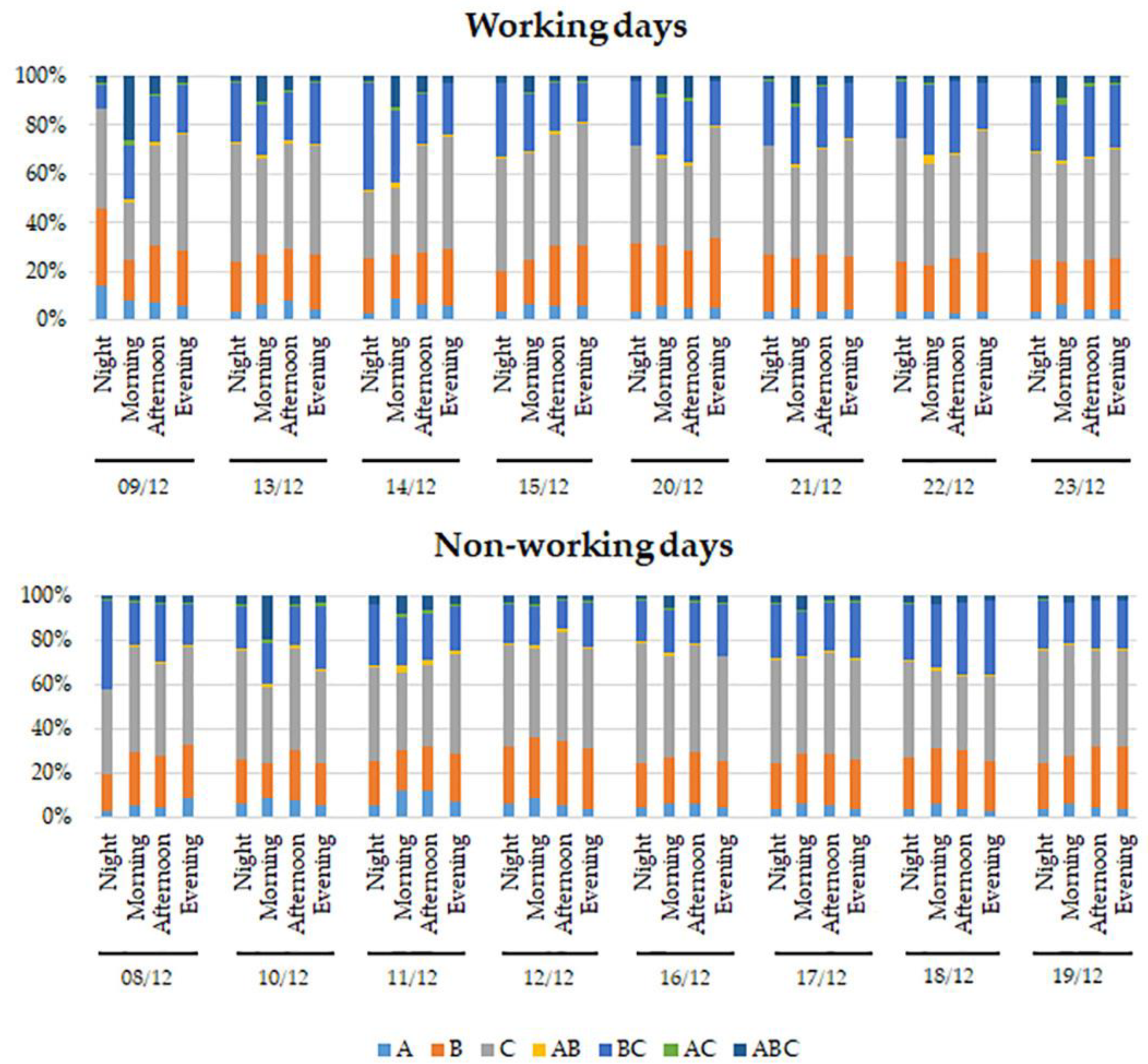
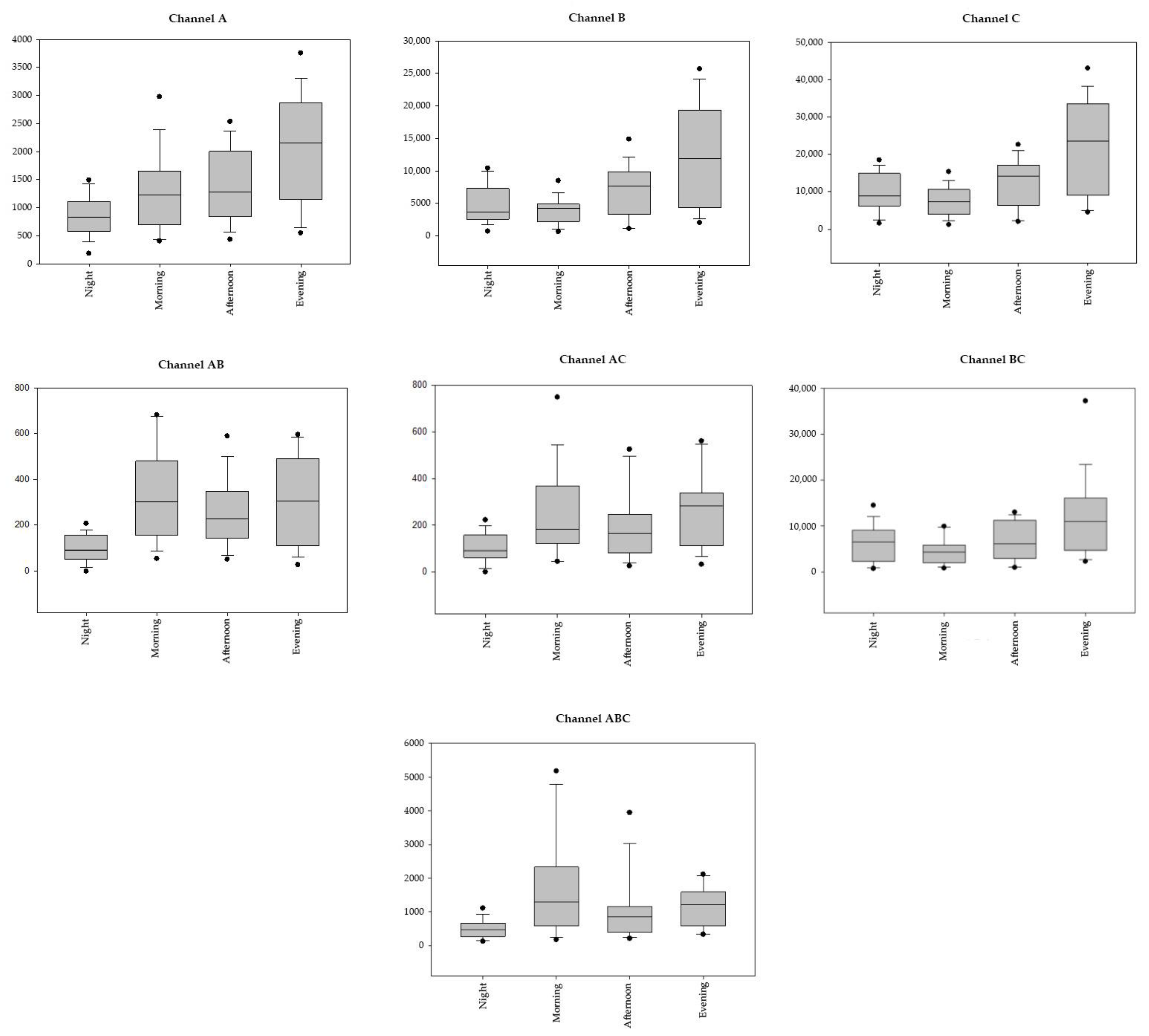
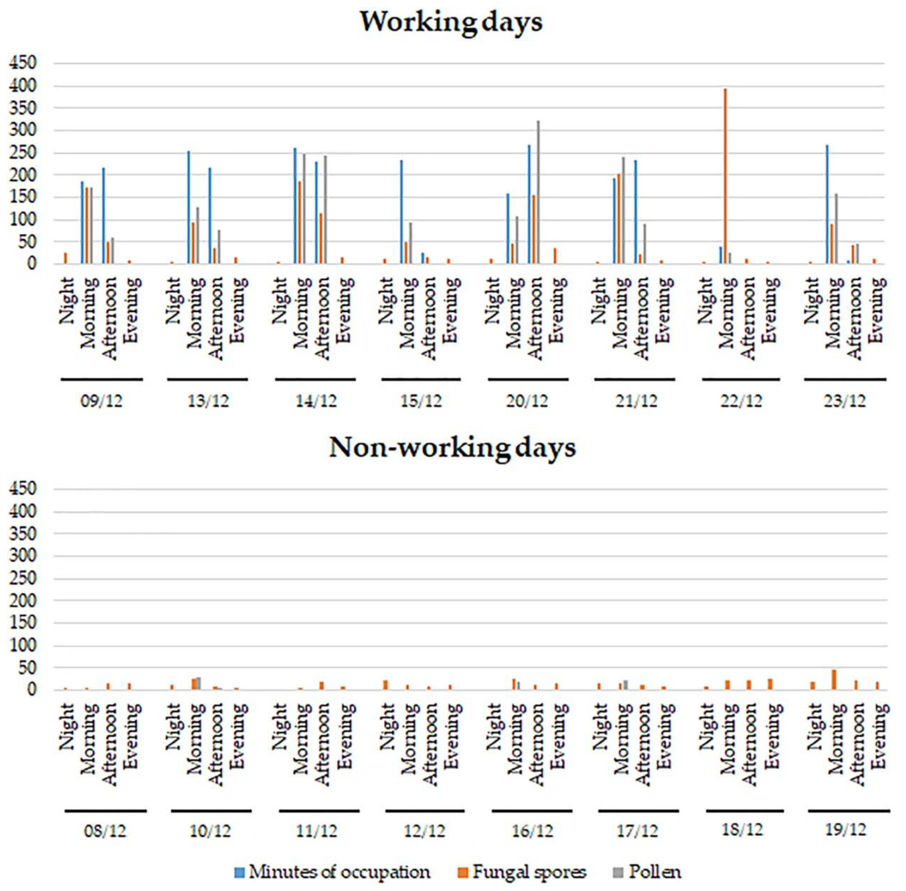
3.2. 6-h and 1-h Distributions of Particles
4. Discussion
5. Conclusions
- A fine temporal resolution of data;
- Lower expense of time for the identification of the bioparticles;
- The unnecessary contribution of an expert in the morphological identification of the several particles types, like pollen or fungal spores;
- A better quantitative evaluation of sampled particles;
- The ability of a single instrument to sample many different bioparticles simultaneously, sparing the need of different sampling methods for each particle type.
Author Contributions
Funding
Institutional Review Board Statement
Informed Consent Statement
Data Availability Statement
Conflicts of Interest
References
- Pearce, D.A.; Alekhina, I.A.; Terauds, A.; Wilmotte, A.; Quesada, A.; Edwards, A.; Dommergue, A.; Sattler, B.; Adams, B.J.; Magalhães, C.; et al. Aerobiology over antarctica—A new initiative for atmospheric ecology. Front. Microbiol. 2016, 7, 16. [Google Scholar] [CrossRef] [PubMed] [Green Version]
- Alsante, A.N.; Thornton, D.C.O.; Brooks, S.D. Ocean aerobiology. Front. Microbiol. 2021, 12, 764178. [Google Scholar] [CrossRef] [PubMed]
- Devadas, R.; Huete, A.R.; Vicendese, D.; Erbas, B.; Beggs, P.J.; Medek, D.; Haberle, S.G.; Newnham, R.M.; Johnston, F.H.; Jaggard, A.K.; et al. Dynamic ecological observations from satellites inform aerobiology of allergenic grass pollen. Sci. Total Environ. 2018, 633, 441–451. [Google Scholar] [CrossRef] [PubMed]
- Glick, S.; Gehrig, R.; Eeftens, M. Multi-decade changes in pollen season onset, duration, and intensity: A concern for public health? Sci. Total Environ. 2021, 781, 146382. [Google Scholar] [CrossRef] [PubMed]
- Haddrell, A.E.; Thomas, R.J. Aerobiology: Experimental considerations, observations, and future tools. Appl. Environ. Microbiol. 2017, 83, e00809-17. [Google Scholar] [CrossRef] [Green Version]
- Singh, A.B.; Mathur, C. An aerobiological perspective in allergy and asthma. Asia Pac. Allergy 2012, 2, 210–222. [Google Scholar] [CrossRef] [Green Version]
- Maddox, R.L. On an Apparatus for collecting atmospheric particles. Mon. Microsc. J. 1870, 3, 286–290. [Google Scholar] [CrossRef]
- Blackley, C. Experimental Researches on the Cause and Nature of Catarrhus Aestivus (Hay Fever, Hay Asthma); Balliere Tindall & Cox: London, UK, 1873. [Google Scholar]
- Oteros, J.; Sofiev, M.; Smith, M.; Clot, B.; Damialis, A.; Prank, M.; Werchan, M.; Wachter, R.; Weber, A.; Kutzora, S.; et al. Building an automatic pollen monitoring network (ePIN): Selection of optimal sites by clustering pollen stations. Sci. Total Environ. 2019, 688, 1263–1274. [Google Scholar] [CrossRef]
- Oteros, J.; Weber, A.; Kutzora, S.; Rojo, J.; Heinze, S.; Herr, C.; Gebauer, R.; Schmidt-Weber, C.B.; Buters, J.T.M. An operational robotic pollen monitoring network based on automatic image recognition. Environ. Res. 2020, 191, 110031. [Google Scholar] [CrossRef]
- Schaefer, J.; Milling, M.; Schuller, B.W.; Bauer, B.; Brunner, J.O.; Traidl-Hoffmann, C.; Damialis, A. Towards automatic airborne pollen monitoring: From commercial devices to operational by mitigating class-imbalance in a deep learning approach. Sci. Total Environ. 2021, 796, 148932. [Google Scholar] [CrossRef]
- Núñez, A.; Amo de Paz, G.; Rastrojo, A.; García, A.M.; Alcamí, A.; Gutiérrez-Bustillo, A.M.; Moreno, D.A. Monitoring of airborne biological particles in outdoor atmosphere. Part 2: Metagenomics applied to urban environments. Int. Microbiol. Off. J. Span. Soc. Microbiol. 2016, 19, 69–80. [Google Scholar] [CrossRef]
- Xu, L.; Pierroz, G.; Wipf, H.M.L.; Gao, C.; Taylor, J.W.; Lemaux, P.G.; Coleman-Derr, D. Holo-omics for deciphering plant-microbiome interactions. Microbiome 2021, 9, 69. [Google Scholar] [CrossRef]
- Darnhofer, B.; Tomin, T.; Liesinger, L.; Schittmayer, M.; Tomazic, P.V.; Birner-Gruenberger, R. Comparative proteomics of common allergenic tree pollens of birch, alder, and hazel. Allergy 2021, 76, 1743–1753. [Google Scholar] [CrossRef] [PubMed]
- Sénéchal, H.; Visez, N.; Charpin, D.; Shahali, Y.; Peltre, G.; Biolley, J.P.; Lhuissier, F.; Couderc, R.; Yamada, O.; Malrat-Domenge, A.; et al. A review of the effects of major atmospheric pollutants on pollen grains, pollen content, and allergenicity. Sci. World J. 2015, 2015, 940243. [Google Scholar] [CrossRef] [Green Version]
- Sedghy, F.; Varasteh, A.R.; Saukian, M.; Moghadam, M. Interaction between air pollutants and pollen grains: The role on the rising trend in allergy. Rep. Biochem. Mol. Biol. 2018, 6, 219–224. [Google Scholar] [PubMed]
- Plaza, M.P.; Alcázar, P.; Oteros, J.; Galán, C. Atmospheric pollutants and their association with olive and grass aeroallergen concentrations in Córdoba (Spain). Environ. Sci. Pollut. Res. 2020, 27, 45447–45459. [Google Scholar] [CrossRef] [PubMed]
- Ortega-Rosas, C.I.; Meza-Figueroa, D.; Vidal-Solano, J.R.; González-Grijalva, B.; Schiavo, B. Association of airborne particulate matter with pollen, fungal spores, and allergic symptoms in an arid urbanized area. Environ. Geochem. Health 2021, 43, 1761–1782. [Google Scholar] [CrossRef]
- Lipiec, A.; Puc, M.; Kruczek, A. Exposure to pollen allergens in allergic rhinitis expressed by diurnal variation of airborne tree pollen in urban and rural area. Otolaryngol. Pol. 2019, 74, 1–6. [Google Scholar] [CrossRef]
- Galveias, A.; Ribeiro, H.; Guimarães, F.; Costa, M.J.; Rodrigues, P.; Costa, A.R.; Abreu, I.; Antunes, C.M. Differential Quercus spp. pollen-particulate matter interaction is dependent on geographical areas. Sci. Total Environ. 2022, 832, 154892. [Google Scholar] [CrossRef]
- Barber, D.; Villaseñor, A.; Escribese, M.M. Metabolomics strategies to discover new biomarkers associated to severe allergic phenotypes. Asia Pac. Allergy 2019, 9, e37. [Google Scholar] [CrossRef]
- Sim, S.; Choi, Y.; Park, H.S. Potential metabolic biomarkers in adult asthmatics. Metabolites 2021, 11, 430. [Google Scholar] [CrossRef]
- Gruzieva, O.; Jeong, A.; He, S.; Yu, Z.; de Bont, J.; Pinho, M.G.M.; Eze, I.C.; Kress, S.; Wheelock, C.E.; Peters, A.; et al. Air pollution, metabolites and respiratory health across the life-course. Eur. Respir Rev. 2022, 31, 220038. [Google Scholar] [CrossRef]
- Yuan, Y.; Wang, C.; Wang, G.; Guo, X.; Jiang, S.; Zuo, X.; Wang, X.; Hsu, A.C.; Qi, M.; Wang, F. Airway microbiome and serum metabolomics analysis identify differential candidate biomarkers in allergic rhinitis. Front. Immunol. 2022, 12, 771136. [Google Scholar] [CrossRef] [PubMed]
- Gehrig, R.; Clot, B. 50 years of pollen monitoring in Basel (Switzerland) demonstrate the influence of climate change on airborne pollen. Front. Allergy 2021, 2, 677159. [Google Scholar] [CrossRef] [PubMed]
- Adams-Groom, B.; Selby, K.; Derrett, S.; Frisk, C.A.; Pashley, C.H.; Satchwell, J.; King, D.; McKenzie, G.; Neilson, R. Pollen season trends as markers of climate change impact: Betula, Quercus and Poaceae. Sci. Total Environ. 2022, 831, 154882. [Google Scholar] [CrossRef]
- Schramm, P.J.; Brown, C.L.; Saha, S.; Conlon, K.C.; Manangan, A.P.; Bell, J.E.; Hess, J.J. A systematic review of the effects of temperature and precipitation on pollen concentrations and season timing, and implications for human health. Int. J. Biometeorol. 2021, 65, 1615–1628. [Google Scholar] [CrossRef] [PubMed]
- Frisk, C.A.; Apangu, G.P.; Petch, G.M.; Adams-Groom, B.; Skjøth, C.A. Atmospheric transport reveals grass pollen dispersion distances. Sci. Total Environ. 2022, 814, 152806. [Google Scholar] [CrossRef]
- Katotomichelakis, M.; Nikolaidis, C.; Makris, M.; Zhang, N.; Aggelides, X.; Constantinidis, T.C.; Bachert, C.; Danielides, V. The clinical significance of the pollen calendar of the Western Thrace/northeast Greece region in allergic rhinitis. Int. Forum. Allergy Rhinol. 2015, 5, 1156–1163. [Google Scholar] [CrossRef]
- Singh, N.; Singh, U.; Singh, D.; Daya, M.; Singh, V. Correlation of pollen counts and number of hospital visits of asthmatic and allergic rhinitis patients. Lung India 2017, 34, 127–131. [Google Scholar] [CrossRef]
- Cariñanos, P.; Alcázar, P.; Galán, C.; Navarro, R.; Domínguez, E. Aerobiology as a tool to help in episodes of occupational allergy in work places. J. Investig. Allergol. Clin. Immunol. 2004, 14, 300–308. [Google Scholar]
- Raulf, M.; Buters, J.; Chapman, M.; Cecchi, L.; de Blay, F.; Doekes, G.; Eduard, W.; Heederik, D.; Jeebhay, M.F.; Kespohl, S.; et al. European Academy of Allergy and Clinical Immunology. Monitoring of occupational and environmental aeroallergens—EAACI Position Paper. Concerted action of the EAACI IG Occupational Allergy and Aerobiology & Air Pollution. Allergy 2014, 69, 1280–1299. [Google Scholar] [CrossRef] [PubMed]
- D’Ovidio, M.C.; Di Renzi, S.; Capone, P.; Pelliccioni, A. Pollen and fungal spores evaluation in relation to occupants and microclimate in indoor workplaces. Sustainability 2021, 13, 3154. [Google Scholar] [CrossRef]
- Lancia, A.; Capone, P.; Vonesch, N.; Pelliccioni, A.; Grandi, C.; Magri, D.; D’Ovidio, M.C. Research progress on aerobiology in the last 30 years: A focus on methodology and occupational health. Sustainability 2021, 13, 4337. [Google Scholar] [CrossRef]
- Pelliccioni, A.; Ciardini, V.; Lancia, A.; Di Renzi, S.; Brighetti, M.A.; Travaglini, A.; Capone, P.; D’Ovidio, M.C. Intercomparison of indoor and outdoor pollen concentrations in rural and suburban research workplaces. Sustainability 2021, 13, 8776. [Google Scholar] [CrossRef]
- Huffman, J.A.; Perring, A.E.; Savage, N.J.; Clot, B.; Crouzy, B.; Tummon, F.; Shoshanim, O.; Damit, B.; Schneider, J.; Sivaprakasam, V.; et al. Real-time sensing of bioaerosols: Review and current perspectives. Aerosol. Sci. Tech. 2020, 54, 465–495. [Google Scholar] [CrossRef] [Green Version]
- Bünger, J.; Schappler-Scheele, B.; Hilgers, R.; Hallier, E. A 5-year follow-up study on respiratory disorders and lung function in workers exposed to organic dust from composting plants. Int. Arch. Occup. Environ. Health 2007, 80, 306–312. [Google Scholar] [CrossRef]
- Niazi, S.; Hassanvand, M.S.; Mahvi, A.H.; Nabizadeh, R.; Alimohammadi, M.; Nabavi, S.; Faridi, S.; Dehghani, A.; Hoseini, M.; Moradi-Joo, M.; et al. Assessment of bioaerosol contamination (bacteria and fungi) in the largest urban wastewater treatment plant in the Middle East. Environ. Sci. Pollut. Res. Int. 2015, 22, 16014–16021. [Google Scholar] [CrossRef]
- Zimmerman, B.; Tafintseva, V.; Bağcıoğlu, M.; Høegh Berdahl, M.; Kohler, A. Analysis of allergenic pollen by FTIR microspectroscopy. Anal. Chem. 2016, 88, 803–811. [Google Scholar] [CrossRef]
- Klimczak, L.J.; von Eschenbach, C.E.; Thompson, P.M.; Buters, J.T.M.; Mueller, G.A. Mixture analyses of air-sampled pollen extracts can accurately differentiate pollen taxa. Atmos. Environ. 2020, 243, 117746. [Google Scholar] [CrossRef]
- Daunys, G.; Šukienė, L.; Vaitkevičius, L.; Valiulis, G.; Sofiev, M.; Šaulienė, I. Clustering approach for the analysis of the fluorescent bioaerosol collected by an automatic detector. PLoS ONE 2021, 16, e0247284. [Google Scholar] [CrossRef]
- Tummon, F.; Arboledas, L.A.; Bonini, M.; Guinot, B.; Hicke, M.; Jacob, C.; Kendrovski, V.; McCairns, W.; Petermann, E.; Peuch, V.H.; et al. The need for Pan-European automatic pollen and fungal spore monitoring: A stakeholder workshop position paper. Clin. Transl. Allergy 2021, 11, e12015. [Google Scholar] [CrossRef]
- Plaza, M.P.; Kolek, F.; Leier-Wirtz, V.; Brunner, J.O.; Traidl-Hoffmann, C.; Damialis, A. Detecting airborne pollen using an automatic.; real-time monitoring system: Evidence from two sites. Int. J. Environ. Res. Public Health 2022, 19, 2471. [Google Scholar] [CrossRef] [PubMed]
- Jiang, C.; Wang, W.; Du, L.; Huang, G.; McConaghy, C.; Fineman, S.; Liu, Y. Field evaluation of an automated pollen sensor. Int. J. Environ. Res. Public Health 2022, 19, 6444. [Google Scholar] [CrossRef] [PubMed]
- Worldwide Map of Pollen Monitoring Stations. Available online: https://oteros.shinyapps.io/pollen_map/ (accessed on 29 August 2022).
- Pöhlker, C.; Huffman, J.A.; Pöschl, U. Autofluorescence of atmospheric bioaerosols—Fluorescent biomolecules and potential interferences. Atmos. Meas. Tech. 2012, 5, 37–71. [Google Scholar] [CrossRef] [Green Version]
- Hernandez, M.; Perring, A.E.; McCabe, K.; Kok, G.; Granger, G.; Baumgardner, D. Chamber catalogues of optical and fluorescent signatures distinguish bioaerosol classes. Atmos. Meas. Tech. 2016, 9, 3283–3292. [Google Scholar] [CrossRef] [Green Version]
- World Health Organization. WHO Global Air Quality Guidelines. Particulate Matter (PM2.5 and PM10), Ozone, Nitrogen Dioxide, Sulfur Dioxide and Carbon Monoxide; World Health Organization: Geneva, Switzerland, 2021; Available online: https://apps.who.int/iris/handle/10665/345329 (accessed on 8 November 2022).
- Annesi-Maesano, I.; Cecchi, L.; Agache, I.; Akdis, C. EAACI Guidelines on Environmental Science for Allergy and Asthma–Recommendations for Pollen-Induced Asthma and Rhinitis. WG Atmospheric. Available online: https://www.eaaci.org/images/Recommendations_EtDts_final.pdf (accessed on 8 November 2022).
- Diem, L.; Neuherz, B.; Rohrhofer, J.; Koidl, L.; Asero, R.; Brockow, K.; Diaz Perales, A.; Faber, M.; Gebhardt, J.; Torres, M.J.; et al. Real-life evaluation of molecular multiplex IgE test methods in the diagnosis of pollen associated food allergy. Allergy 2022, 77, 3028–3040. [Google Scholar] [CrossRef]
- Raulf, M. Allergen component analysis as a tool in the diagnosis and management of occupational allergy. Mol. Immunol. 2018, 100, 21–27. [Google Scholar] [CrossRef]
- Radzikowska, U.; Baerenfaller, K.; Cornejo-Garcia, J.A.; Karaaslan, C.; Barletta, E.; Sarac, B.E.; Zhakparov, D.; Villaseñor, A.; Eguiluz-Gracia, I.; Mayorga, C.; et al. Omics technologies in allergy and asthma research: An EAACI position paper. Allergy 2022, 17, 2888–2908. [Google Scholar] [CrossRef]
- Pointner, L.; Bethanis, A.; Thaler, M.; Traidl-Hoffmann, C.; Gilles, S.; Ferreira, F.; Aglas, L. Initiating pollen sensitization—Complex source, complex mechanisms. Clin. Transl. Allergy 2020, 10, 36. [Google Scholar] [CrossRef]
- D’Ovidio, M.C.; Capone, P.; Lancia, A.; Melis, P.; Tranfo, G.; Grandi, C.; Annesi-Maesano, I. The need of integrated tools for the study of occupational exposure to allergens. Acta Sci. Med. Sci. 2022, 6, 108–118. [Google Scholar]
- Ravindra, K.; Goyal, A.; Mor, S. Pollen allergy: Developing multi-sectorial strategies for its prevention and control in lower and middle-income countries. Int. J. Hyg. Environ. Health 2022, 242, 113951. [Google Scholar] [CrossRef] [PubMed]
- Geoportale cartografico - Città metropolitana di Roma Capitale. Available online: http://websit.cittametropolitanaroma.it/DescriviMappa.aspx?i=7 (accessed on 12 January 2021).
- Perring, A.; Schwarz, E.; Baumgardner, J.P.; Hernandez, D.; Spracklen, M.T.; Heald, D.V.; Gao, R.S.; Kok, G.; Mcmeeking, G.; Fahey, J.; et al. Airborne observations of regional variation in fluorescent aerosol across the United States. J. Geophys. Res. Atmos. 2015, 120, 1153–1170. [Google Scholar] [CrossRef]
- Li, J.; Wan, M.P.; Schiavon, S.S.; Tham, K.W.; Zuraimi, S.; Xiong, J.; Fang, M.; Gall, E. Size-resolved dynamics of indoor and outdoor fluorescent biological aerosol particles in a bedroom: A one-month case study in Singapore. Indoor Air 2020, 30, 942–954. [Google Scholar] [CrossRef] [PubMed]
- Addor, Y.S.; Baumgardner, D.; Hughes, D.; Newman, N.; Jandarov, R.; Reponen, T. Assessing residential indoor and outdoor bioaerosol characteristics using the ultraviolet light-induced fluorescence-based wideband integrated bioaerosol sensor. Environ. Sci. Process. Impacts 2022, 24, 1790–1804. [Google Scholar] [CrossRef]
- Wingert, L.; Debia, M.; Hallé, S.; Marchand, G. Occupational microbial risk among embalmers. Atmosphere 2022, 13, 1281. [Google Scholar] [CrossRef]
- Tummon, F.; Adamov, S.; Clot, B.; Crouzy, B.; Gysel-Beer, M.; Kawashima, S.; O’Connor, D. A first evaluation of multiple automatic pollen monitors run in parallel. Aerobiologia 2021, 1–16. [Google Scholar] [CrossRef]


| Date | Day Type | Total Particles | Fluorescent Particles | A | B | C | AB | BC | AC | ABC |
|---|---|---|---|---|---|---|---|---|---|---|
| 8 December 2021 | NWD | 367,709 | 53,836 | 2623 | 11,425 | 22,456 | 343 | 15,420 | 286 | 1283 |
| 9 December 2021 | WD | 591,041 | 71,148 | 5346 | 15,593 | 27,694 | 838 | 13,682 | 751 | 7244 |
| 10 December 2021 | NWD | 231,777 | 36,912 | 2501 | 6946 | 16,152 | 403 | 7990 | 368 | 2552 |
| 11 December 2021 | NWD | 166,621 | 26,213 | 2202 | 5365 | 11,038 | 410 | 5640 | 278 | 1280 |
| 12 December 2021 | NWD | 816,042 | 111,532 | 4964 | 30,819 | 50,443 | 855 | 21,156 | 464 | 2831 |
| 13 December 2021 | WD | 585,286 | 99,779 | 4943 | 22,112 | 43,494 | 845 | 23,397 | 655 | 4333 |
| 14 December 2021 | WD | 974,774 | 156,781 | 9097 | 34,142 | 58,986 | 1753 | 42,973 | 1230 | 8600 |
| 15 December 2021 | WD | 752,790 | 117,279 | 6712 | 25,646 | 54,904 | 1104 | 24,518 | 920 | 3475 |
| 16 December 2021 | NWD | 985,689 | 135,856 | 6876 | 29,047 | 65,128 | 1040 | 28,647 | 1007 | 4111 |
| 17 December 2021 | NWD | 803,036 | 139,289 | 5396 | 31,413 | 62,933 | 957 | 33,681 | 842 | 4067 |
| 18 December 2021 | NWD | 946,350 | 198,500 | 6427 | 47,446 | 75,008 | 1379 | 62,617 | 1020 | 4603 |
| 19 December 2021 | NWD | 982,174 | 181,196 | 7343 | 47,260 | 82,387 | 1234 | 38,397 | 863 | 3712 |
| 20 December 2021 | WD | 1,179,742 | 179,236 | 8501 | 48,288 | 72,927 | 1683 | 39,276 | 1257 | 7304 |
| 21 December 2021 | WD | 1,003,323 | 179,836 | 7304 | 40,439 | 77,992 | 763 | 44,118 | 1144 | 8076 |
| 22 December 2021 | WD | 742,422 | 134,563 | 4529 | 30,032 | 62,616 | 1231 | 32,773 | 319 | 3063 |
| 23 December 2021 | WD | 569,872 | 115,834 | 5042 | 23,447 | 49,159 | 1071 | 30,833 | 1353 | 4929 |
| Total | 11,698,648 | 1,937,790 | 89,806 | 449,420 | 833,317 | 15,909 | 465,118 | 12,757 | 71,463 | |
| Mean | 731,165 | 121,112 | 5613 | 28,089 | 52,082 | 994 | 29,070 | 797 | 4466 |
| A | B | C | AB | BC | AC | ABC | |
|---|---|---|---|---|---|---|---|
| Evening vs. Night | Yes | Yes | Yes | Yes | Yes | Yes | Yes |
| Evening vs. Morning | Yes | Yes | Yes | No Test | Yes | No Test | No Test |
| Evening vs. Afternoon | Yes | Yes | Yes | No Test | Yes | No | No Test |
| Afternoon vs. Night | Yes | No Test | No Test | Yes | No Test | Yes | Yes |
| Afternoon vs. Morning | No | No | No | No | No | No Test | No |
| Morning vs. Night | Yes | No Test | No Test | Yes | No Test | Yes | Yes |
| WDs vs. NWDs Comparison | |||||
|---|---|---|---|---|---|
| Channel | Day | Median | Day Section | ||
| A | WDs | 1573.5 | Night | p = 0.38 ** | |
| NWDs | 963 | p= 0.011 * | Morning | p= 0.017 ** | |
| Afternoon | p = 0.07 ** | ||||
| Evening | p = 0.804 ** | ||||
| B | WDs | 7195 | Night | p = 0.227 ** | |
| NWDs | 4045.5 | p= 0.030 * | Morning | p= 0.042 ** | |
| Afternoon | p = 0.362 ** | ||||
| Evening | p = 0.645 ** | ||||
| C | WDs | 14,184.5 | Night | p = 0.529 ** | |
| NWDs | 7370.5 | p= 0.036 * | Morning | p = 0.075 ** | |
| Afternoon | p = 0.149 ** | ||||
| Evening | p = 0.754 ** | ||||
| AB | WDs | 281 | Night | p = 0.813 ** | |
| NWDs | 154.5 | p = 0.099 * | Morning | p< 0.001 ** | |
| Afternoon | p = 0.213 ** | ||||
| Evening | p = 0.557 ** | ||||
| BC | WDs | 7461.5 | Night | p = 0.215 ** | |
| NWDs | 3783 | p= 0.021 * | Morning | p= 0.004 ** | |
| Afternoon | p = 0.161 ** | ||||
| Evening | p = 0.442 * | ||||
| AC | WDs | 194 | Night | p = 0.949 ** | |
| NWDs | 126 | p= 0.041 * | Morning | p< 0.001 * | |
| Afternoon | p = 0.105 * | ||||
| Evening | p = 0.382 ** | ||||
| ABC | WDs | 1115 | Night | p = 0.928 ** | |
| NWDs | 528 | p= 0.005 * | Morning | p= 0.005 * | |
| Afternoon | p= 0.005 * | ||||
| Evening | p = 0.375 ** | ||||
| Pollen + Spores | Spores | Pollen | |
|---|---|---|---|
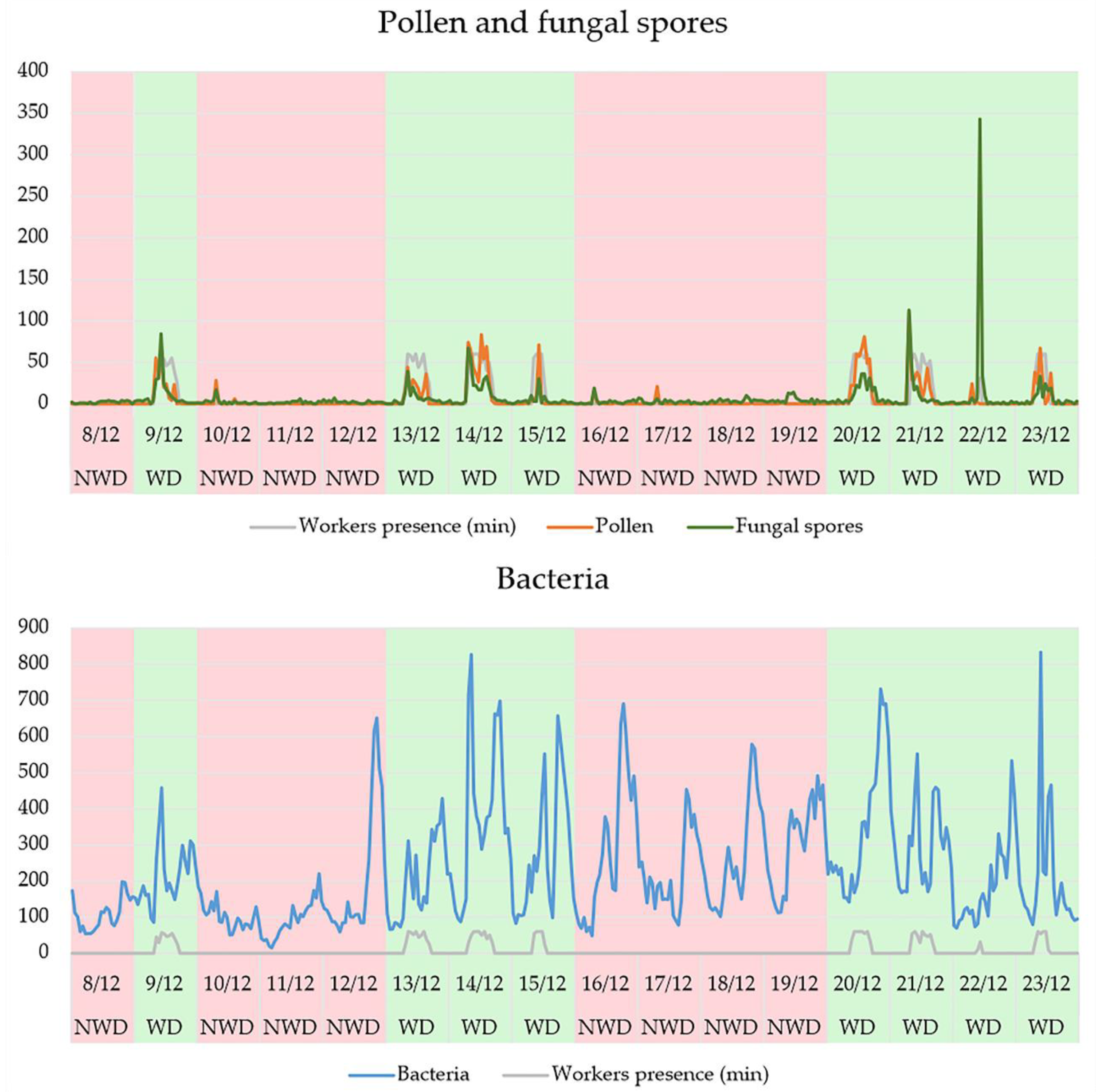
| WHs vs. NWHs | p < 0.001 | p < 0.001 | p < 0.001 |
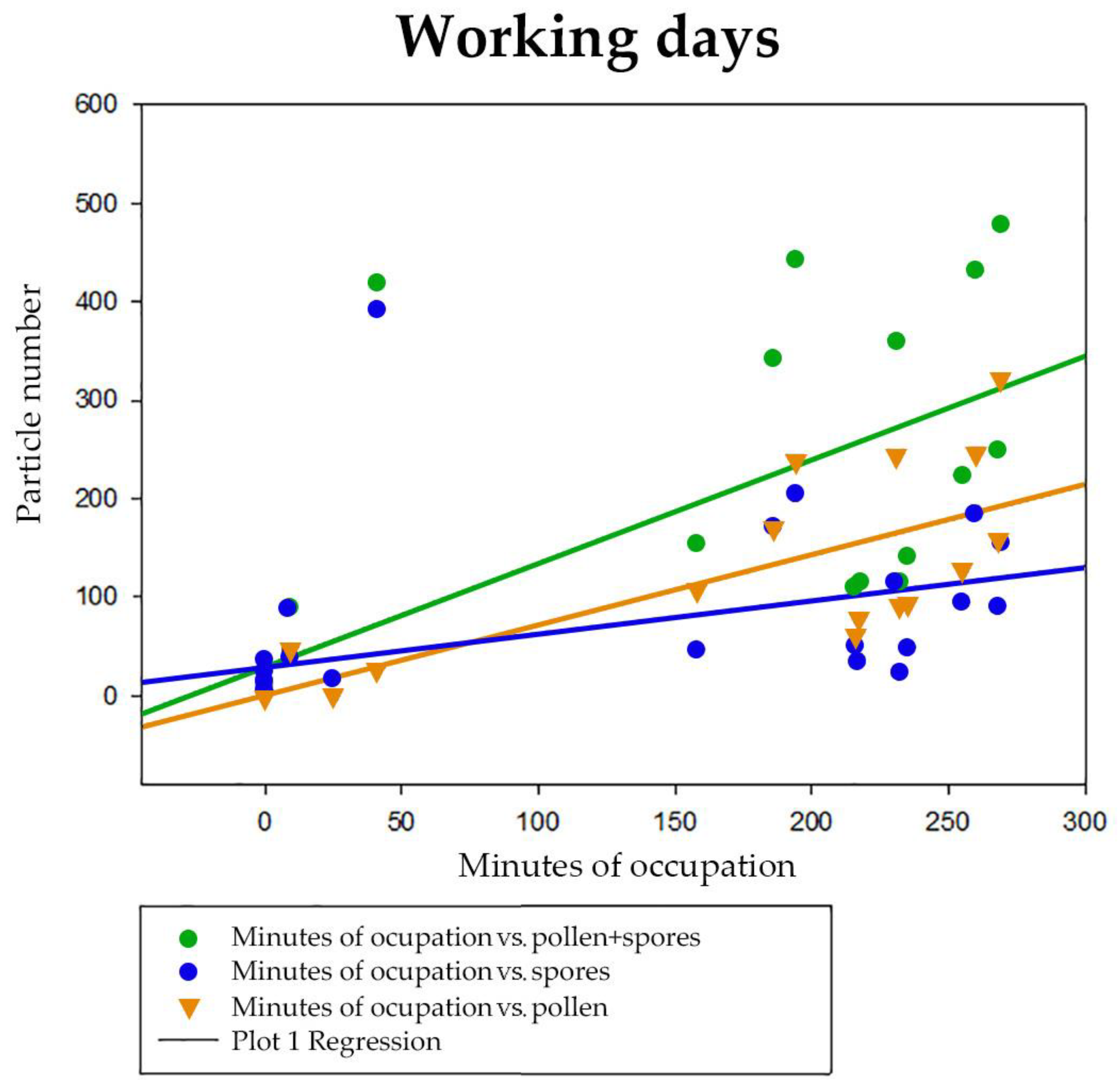
| WDs vs. NWDs | p = 0.047 | p = 0.031 | p = 0.035 |
Disclaimer/Publisher’s Note: The statements, opinions and data contained in all publications are solely those of the individual author(s) and contributor(s) and not of MDPI and/or the editor(s). MDPI and/or the editor(s) disclaim responsibility for any injury to people or property resulting from any ideas, methods, instructions or products referred to in the content. |
© 2023 by the authors. Licensee MDPI, Basel, Switzerland. This article is an open access article distributed under the terms and conditions of the Creative Commons Attribution (CC BY) license (https://creativecommons.org/licenses/by/4.0/).
Share and Cite
Lancia, A.; Gioffrè, A.; Di Rita, F.; Magri, D.; D’Ovidio, M.C. Aerobiological Monitoring in an Indoor Occupational Setting Using a Real-Time Bioaerosol Sampler. Atmosphere 2023, 14, 118. https://doi.org/10.3390/atmos14010118
Lancia A, Gioffrè A, Di Rita F, Magri D, D’Ovidio MC. Aerobiological Monitoring in an Indoor Occupational Setting Using a Real-Time Bioaerosol Sampler. Atmosphere. 2023; 14(1):118. https://doi.org/10.3390/atmos14010118
Chicago/Turabian StyleLancia, Andrea, Angela Gioffrè, Federico Di Rita, Donatella Magri, and Maria Concetta D’Ovidio. 2023. "Aerobiological Monitoring in an Indoor Occupational Setting Using a Real-Time Bioaerosol Sampler" Atmosphere 14, no. 1: 118. https://doi.org/10.3390/atmos14010118