1. Introduction
The air quality measurement is essential in transforming shipping into environmentally friendly activities [
1]. The maritime transportation demand continues to grow, and the emission concentration needs to be reduced to comply with the level stipulated in [
2,
3]. In this respect, the maximum allowable concentrations are introduced to keep the air quality on an acceptable level in the populated harbour areas [
4,
5].
Additionally, a significant impact on air quality is seen during ship navigation, queuing, approaching, terminal processing, and departure [
6,
7]. Recent studies show that the particulate matter and nitrogen oxides from shipping [
8] potentially affected the surrounding area of the ports. The relatively high sulphur content in marine fuels leads to elevated sulphur dioxide emissions [
9].
In numerous studies, the bottom-up approach is most often used, considering manoeuvring and hoteling as main ship activities in the port [
10,
11,
12]. Since the operational activity of the ship reflects the status of ship engines and the corresponding emissions rate, the anchorage is considered an essential operational mode to be analysed [
13]. Ships at anchor impact the environment through air emissions, noise pollution, seabed scouring, liquid waste streams, solid waste, and antifouling paints [
14].
The energy efficiency design index (EEDI) is used as an essential design factor to enhance the ship energy efficiency [
15,
16,
17], and its maximum required level was stipulated in [
18]. The automatic identification system (AIS) ship data [
19,
20] facilitates ship energy efficiency and air pollution analyses.
Several models are used to simulate the atmospheric dispersion of pollutants from ships under movement. The study presented in [
21] compares commonly used line source (LS), fixed point source (FPS), and the newly proposed moving point source (MPS) model. The MPS accounts for the speed and direction to update the ship positions and estimates the emission dispersion at different simulation times. The main conclusion is that the MPS has great potential for a real-time simulation of the shipping emission dispersion using AIS ship position data.
The Gaussian dispersion models were developed and widely used for modelling emission propagation [
22,
23], where the relationship between the emission rate, accounting for meteorological conditions, can be defined by the vertical and the crosswind models [
24,
25,
26], estimating the air pollution concentration for one specific period.
A recent study performed in [
27,
28] used the Gaussian dispersion model to define the pollution concentration in crowded port areas and other reference points. The emission concentration at the receptors accounted for the wind speed, horizontal and vertical dispersion parameters as a function of the geographical location of the ships, effective emission height, and weather conditions. A target level is defined conditional to failure cause and mode. It is used to identify safety calibration factors in defining the most suitable location and distance from the crowded zones and the source of pollution represented by the ships queuing at the seaport.
The present work develops a multidisciplinary approach for evaluating the air pollution and economic impact of ships operating in the port of Varna to identify the most efficient berth terminal operation. The primary contribution of this work is joining well-established methods to identify the most efficient berth terminal operation, accounting for air pollution and the cost associated with the ship and terminal operations. Several simplifications and parameter values in the present study are assumed for the port of Varna, which are not essential for the approach but are needed to demonstrate its capability. The air quality control and collection of data in this area for the port of Varna are very much delayed concerning other European ports. The present work develops an approach based on limited information and provides a credible solution.
2. Port and Ships Characteristics
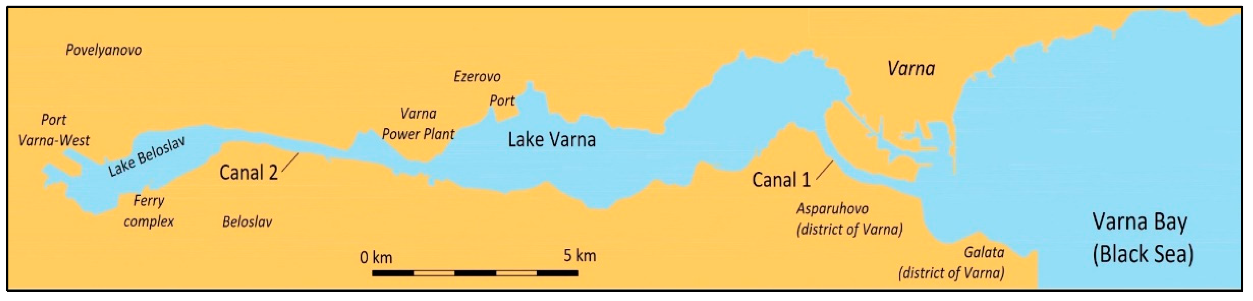
This study analyses the dry cargo ships’ operation activity in the port of Varna, located on the west coast of the Black Sea. The terminals are built in Varna West port, approximately 26 km from the Black Sea coast, passing through a canal. The cargo loading and unloading are performed in three existing terminals, where the dry cargo ships are processed.
A 12 m-deep navigable canal operates from the Black Sea to the lake of Varna and Beloslav and ends at the port of Varna West and the railroad ferry terminal (
https://commons.wikimedia.org/wiki/File:Varna-Devnya_canal_map-AR.gif (accessed on 5 July 2022)). Several small ports are encountered on the north shore. The canal used for ships operating from the seaport to the port of Varna West is shown in
Figure 1.
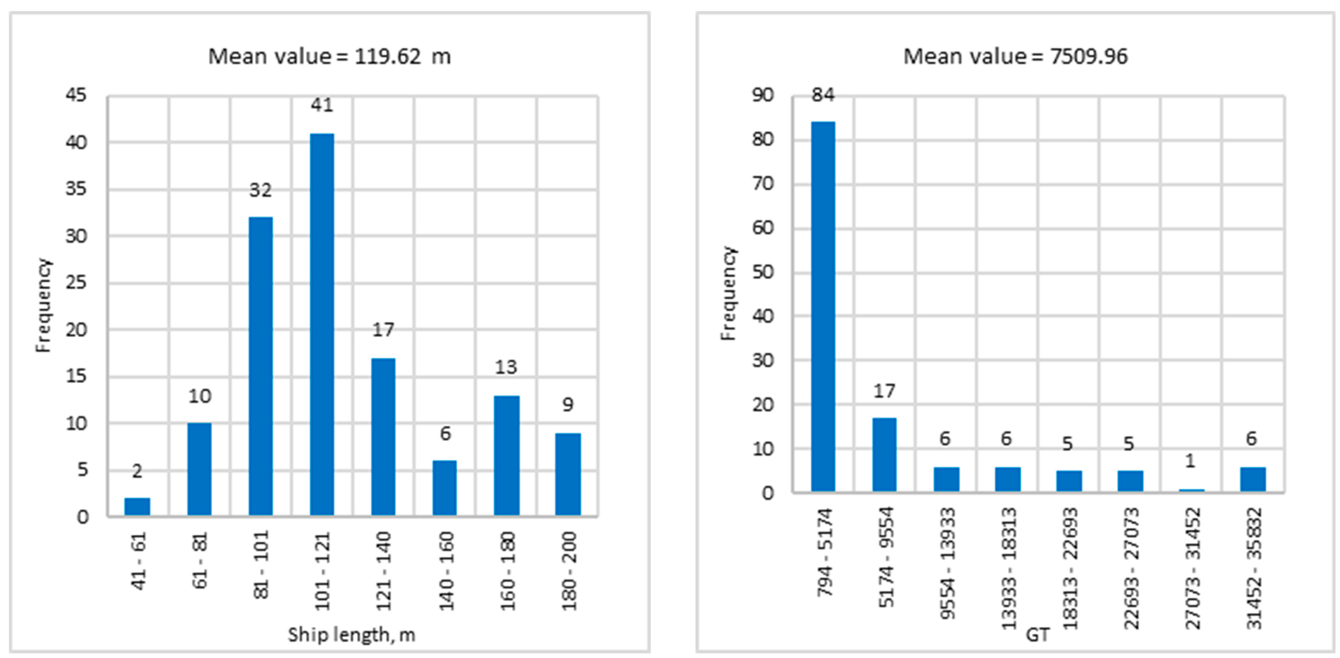
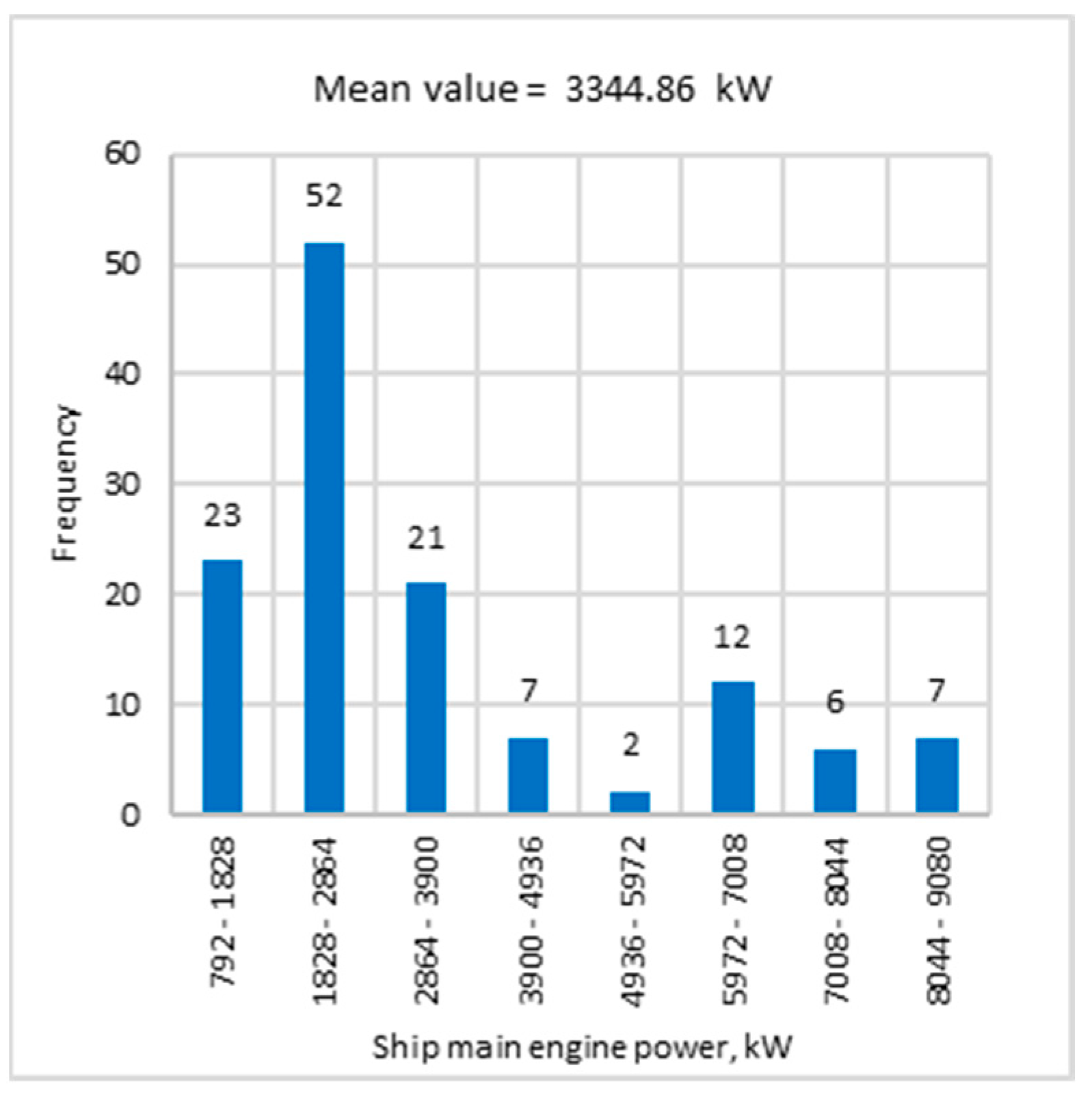
The ship’s main characteristics for the present study include the ship’s length, GT, and engine power. The average length of the arriving ship in the seaport of Varna is 119.62 m, with a GT of 7509.96, and the ship’s main propulsion power is 3344.86 Kw. The ship length (mean value = 119.62 m, St. Dev. = 34.9 m) and GT (mean value = 7509.96, St. Dev. = 8594.93) histograms are shown in
Figure 2, and ship engine power (mean value = 3344.86 Kw, St. Dev. = 2164.44 Kw) in
Figure 3, respectively. The auxiliary power is assumed to be 33% of the main power.
The essential factors that define the ship’s operation in the port are the delays while waiting to be processed, where the ship’s arrival and berth service time affect these delays. The dry cargo ship’s arrival in ports is irregular, and arriving in the port may directly go to the berth or need to wait until a berth becomes available. However, this depends on a number of factors, such as cargo availability and the respective transport used for transhipment, as well as purely organisational reasons and proper documentation. The berth service time depends on the cargo transported by ships and the capacity of the port terminals for handling and storing cargo. In addition to the arrival and berth service time, the ship spends some more time queuing, approaching, departing, waiting at berth, and berth service time. The analysis of ship circulation and cargo handling is a very complex problem, and the queuing theory can be employed.
First, a ship arrives at the seaport anchorage area, where the interarrival time is defined as the time elapsed between the arrival of the ship and one following it to the seaport. The ship’s time between arrivals is assumed to follow a Poisson distribution for the arrival rate.
To predict the number of ships encountered in a port in a time window, a day, the arrival pattern of ships and the berth service time for handling cargo are fitted to an exponential distribution [
29].
The anchoring or queuing time is the time elapsed waiting in the seaport before the ship approaches the berth. The approaching time is the time needed for ships to move from the seaport to the berth and the returning time is the time required for the ship to return from the berth to the seaport. The berth service time is the time for the mooring operation of ships, waiting, and working time. The berth working time is the time for loading and unloading when the ship is at berth. The waiting time is the time difference between when the actual service starts and the arriving time at the berth. The service time of a ship at a berth is assumed to follow an exponential distribution.
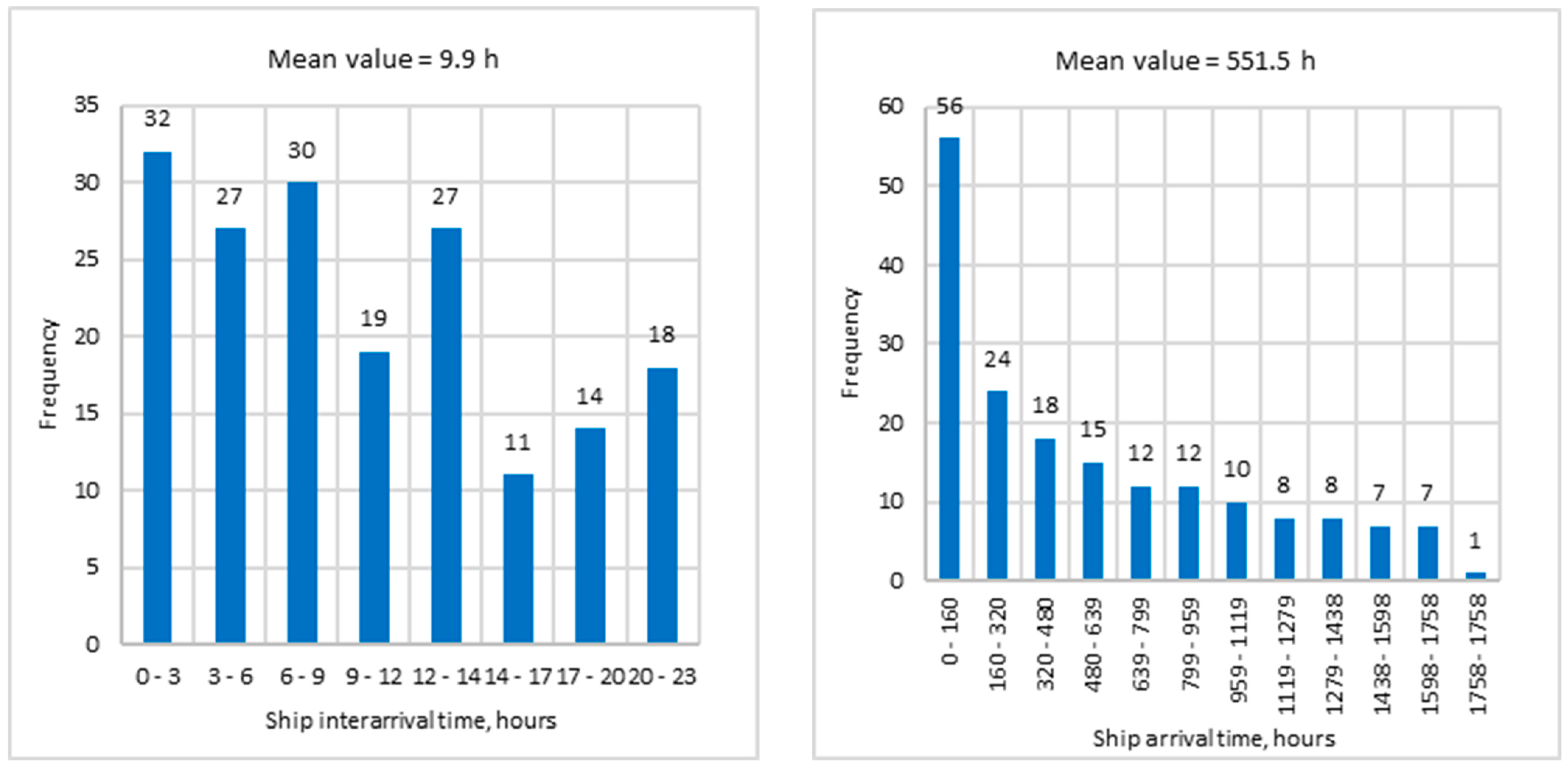
The interarrival and arrival time histograms, based on the collected information for the dry cargo ships in the seaport used in the present study, are shown in
Figure 4.
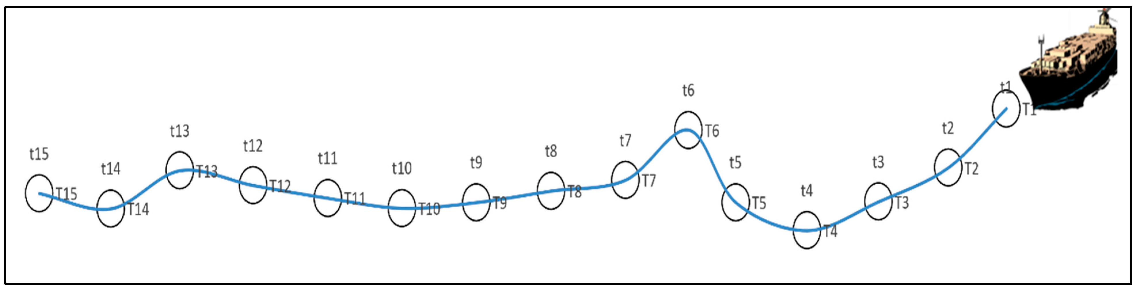
The approaching and departure times are defined using the circulation speed in different trajectories and employing the Monte Carlo simulation following the exponential distribution. The assumed speed from trajectory 1 to 6 and 11 to 15 is 4.12 m/s, and from trajectory 7 to 14 is 6.18 m/s. The spatio-temporal path for an ongoing moving ship is shown in
Figure 5.
The average approaching and departure time is 1.6 h. The service time is defined by using the average cargo
DW of the dry cargo ship of 6400 tonnes/ship leading to 8800 tonnes/day to be processed by the three terminals at an average service time of 56 h/ship, and employing the Monte Carlo simulation [
30], considering the exponential distribution is followed.
3. Ship Gas Emission
The gas emissions of ships operating in the port of Varna analysed are of NOx, SO2, and PM10, and are defined based on the installed propulsion, auxiliary engine power, and used fuel type. It is assumed that the propulsion and the auxiliary engines use marine diesel oil (MDO).
The engine load factors are estimated as a function of the power output. The engine time factors are defined using the time spent in a specific operational activity relative to the total duration. The factors assumed here are
, which is the propulsion engine load factor, and
is the auxiliary engine load factor. During different activities in the voyage, the load factors are assumed as
= 80%,
,
,
,
for the propulsion engine, and
and
for auxiliary engine, respectively [
28].
The emissions depend on several factors, including propulsion, auxiliary engine power, and the fuel types of the ship. The emission factors [
2] used in the analysis are
, and
The gas emission rate,
, is estimated for
th ship by multiplying the time spent in
th activities,
, with the sum of the installed propulsion,
, and auxiliary,
engine power, load factors for propulsion,
, and auxiliary
engine and operational and emission factors for propulsion,
and auxiliary,
, engines. The emissions for the
th operating mode [
31] are calculated as:
where the index
is associated with queuing, approaching, waiting, service at berth, and returning to the seaport.
The concentrations emission rate, as a function of meteorological conditions, is estimated using the crosswind Gaussian dispersion model [
24,
25,
26] for one specific period in one geographical location as:
where
,
are the dispersion coefficients in the crosswind and vertical directions,
and
are the longitudinal and transverse distances from the source,
is the wind speed, and
is the effective stack height, showing that the concentration in each point of the space is proportional to the emission rate
and inversely proportional to the wind speed
. The dispersion coefficients
and
are related to a receptor’s geographical location position and weather conditions.
This model is already employed to analyse the most appropriate location for the seaport [
27] and air pollution from short sea shipping [
28].
4. Moving Ship Pollution
The pollution generated by the ongoing moving ships in the canal, from the seaport to the terminal, is estimated using the Gaussian dispersion model. The emitted pollution from the time step ship moving is integrated into each simulation step. For the ship as a point source of pollution, a Gaussian dispersion model is implemented to define the pollutants released at any individual time step interval . The transport of pollutants is only modelled on the ground level.
The ship route is segmented into trajectories. The trajectory is defined by restricting the path lifespan into a specific time interval,
, where the moving ship passes through the spatio-temporal route (STR) segments, as seen in
Figure 5. The ship can travel many trajectories, one after the other. Initially, the ship is queuing at the seaport and starts approaching the terminal following the trajectory
to
and returns by trajectory
to
.
The moving ship accumulates concentrations in the receptors along the route. The emission concentration at the receptor points of the surrounding area of the port is estimated as a sum of the moving ship, seeing as a point polluting source when travelling in the canal and as a ship fixed polluting point when the ships are at the seaport and terminal is defined as:
where
is the receptor pollution concentration at the time
,
is the receptor pollution concentration at the time
,
is the pollution concentrations contributed from the ship emission sources at the seaport,
is the concentrations contributed from the ship emission sources at the terminal, and
. The total numbers in the sums are the pollution concentrations contributed by the moving ship emission sources at seaport
J, terminal
K, and canal
L.
The time–space function that describes the ship’s position is defined over the whole life span, and it is a function of three parameters related to turning angle, start, and end time, which needs to be updated at any time
and kept constant in the trajectory. The ship as a source of the pollution position will be more realistic when the time step
is smaller. For the time step
, when the ship goes from one point to another through the canal, the estimation of the ship’s virtual position takes the time factor into account:
where
is the speed between
points and
,
are the increments defined as:
The ship’s speed and direction are only updated at each point, assuming that the ship is moving in a straight line or a curve with a constant speed in the trajectory. This simplifies the problem since the moving ship changes the parameters frequently. The present model is used to simulate the dispersion of ship emissions in the seaport, canal, and terminal. The simplified simulation includes a total number of twenty dry cargo ships of different sizes, GT, and engine power.
5. Port Services
Ship activities in port will define the pollution level in the surrounding areas depending on ship service and operating time duration while in port. High port activities can produce a high air pollution concentration.
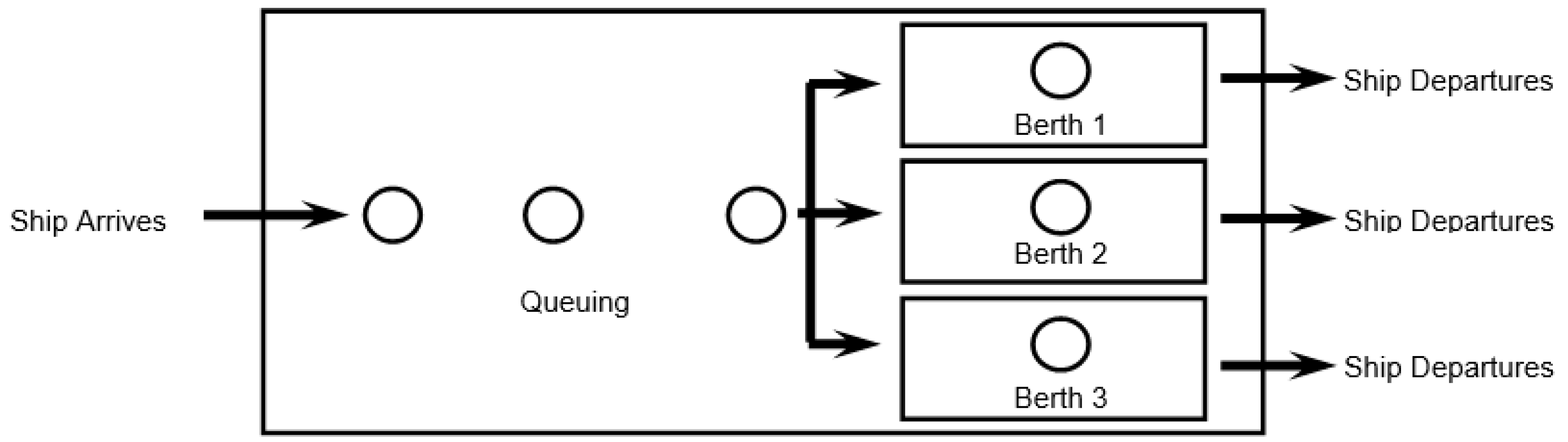
The existing service area of the port is divided into terminals. The queueing theory [
32] is employed to analyse the movement of ships arriving and anchored at the seaport in a single queue. Three parallel cargo berths serve the ships. If a ship arrives at the seaport and the cargo loading and unloading berth is busy serving another ship, the arrived ship joins the end of the queue at the seaport. The service times associated with the arrival, queuing, approaching, waiting, berth service, and departing of the ships are independent and follow the negative exponential distribution function.
The process is considered as a Poisson one, in which the number of arrivals in a specified period is distributed according to the Poisson distribution with a mean arrival rate , representing the number of ships arrived per day. The arrival time determines how the ships are chosen from the queuing line to start service. It can be distinguished as the “First Come First Served”, “Last Come First Served”, or “Service in Random Order”. The departure deals with the ship leaving the terminal. It is also assumed that the queue length is unlimited, relating to the fact that when a ship arrives and finds a long queue, it does not leave the port and join the line.
The pattern of the berth service time distribution is assumed to be exponential with a mean value of , where is the average ship served per day. The approaching and returning patterns of ships are also assumed to be probabilistic variables following the exponential distribution.
The present study assumes that the service times are exponentially distributed, corresponding to an
queueing system of three parallel canals, defined by three cargo servicing berths (
Figure 6).
The objective is to identify the most efficient berth services for the number of ships circulating in the port to minimise the pollution they generate, which will be assessed through the queuing processes and Gaussian air pollution simulations and the cost associated with operation in the port.
The queuing system state at time is defined by the number of ships in the system, which is modelled as a regenerative stochastic process. The regeneration times, describing the interarrival, queuing, approaching, berth service, and departing, are defined as the ship’s interarrival times, at the seaport, the approaching time when the ship moves from the seaport to the berth, , the time the ship is waiting at the berth for the beginning of the service, , the time the ship is served at the berth at the cargo terminal, , and the time for departing, . It is also assumed that the system is initially empty, and the berths are ready to receive ships to be served.
Several events cover the entire process: interarrival, approaching (the passage between the seaport to the berth for loading and unloading operations), waiting at berth, berth servicing, and departure events. If a new ship joins the queuing line at the interarrival event, the number of ships in the system increases by one, and if a ship arrives in the return event, the total number of ships decreases by one.
An interarrival event triggers the next event at a time . If the system is empty at time at the interarrival event, then the interarrival triggers an approaching event . The next step is waiting at the berth event then the transition triggers a service event , provided that there is at least one ship in the line to be served, and finally, the service triggers a departing event at .
At any moment, no more than four events are scheduled: the current event, and at most four future events (interarrival; or interarrival and an approaching; or interarrival, approaching, and waiting-servicing; or interarrival, approaching, waiting-servicing, and departing).
The simulation is stopped at the time when the last ship enters the berth for serving. The utilisation rate for each berth,
is the percentage of server usage defined as [
33]:
The average time a ship waits in the queue is defined as [
33]:
where
is the number of service canals accounting for the average service level in each canal,
is the probability of zero ships in the port is defined as [
33]:
the average number of ships that are waiting in the queue is defined as [
33]:
the average waiting time a ship spends in the port is defined as [
33]:
the average number of ships in the port is defined as [
33]:
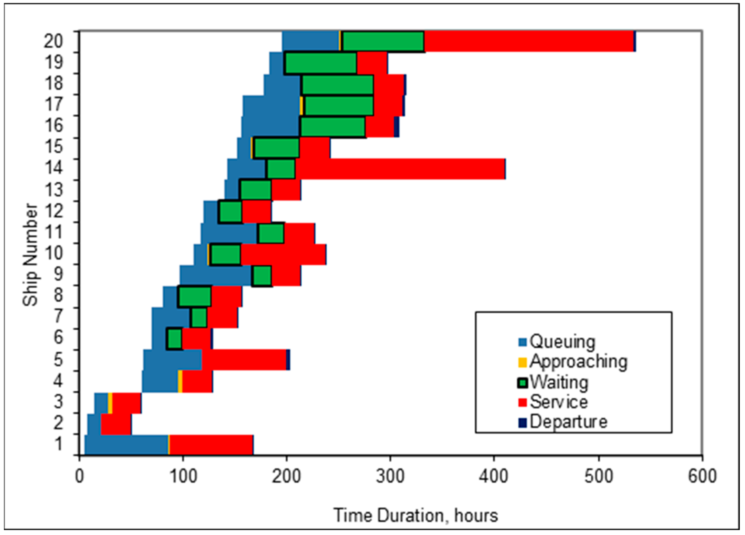
To model a multi-terminal, each ship’s arrival, queuing, approaching, waiting, servicing, and departure are considered. The logic is to verify which event occurs first. The simulation starts with the generation of the first event (i.e., the arrival time of the first ship). Once the ship arrives, the ship either joins the queue or approaches the terminal, depending on the terminal availability. If there is more than one idle terminal, the ships randomly go to one of them. The last step is to define the service and departure time and to return to the next arrival time. The time duration of the 20 dry-cargo ships circulating in the port of different phases, including queuing, approaching, waiting, service, and departure of the ship in the port, is given in
Figure 7.
6. Cost Estimates
The port activity cost comprises the berth service cost,
, and the ship-associated cost,
. The berth service cost includes the investment, maintenance, services of the berth, and stacking yard. The
n-berth investment cost,
is defined as:
where
is the cost of berth area,
is the number of berths,
and
are the length and berth of the
ith berth. The
n-berth equivalent uniform annual cost,
is estimated as:
where
is the berth service life and
is the interest rate. The total equivalent uniform annual cost,
of
n-berths, and surrounding space and equipment is calculated as:
where the maintenance cost
is taken as a percentage of the investment cost.
The waiting cost is due to the ship queuing for service at the seaport, entering the cargo port and waiting in the terminal to start handling operation, as estimated by ship opportunity cost. The ship waiting cost,
, for the average ships in the queue,
, is defined as:
where
is the average cargo
DW of the ship served in the port, and
is the ship cargo revenue.
The goods opportunity cost,
and depreciation,
, define the cargo waiting cost as a function of the cargo value:
where the congestion cost,
, €/tonne/day is estimated as:
where
is the price of the cargo.
The total waiting cost, is defined as the sum of the ship and the cost of cargo waiting time.
The long-term prediction of the concentration is estimated, considering that the analysis period is composed of a sum of a series of short-time stationary conditions without considering the possible correlation between the sequence conditions.
It is assumed that
is the reduction factor of the air contamination from the
jth ship, when
j = 1,…
, and
= (
,…,
) ∈ [0,1], and also that the total cost
of cleaning is a linear function of
defined as:
where
is the cost of cleaning air pollution. The maximum allowable concentrations,
assumed as
= 20 μg/m
3,
= 20 μg/m
3, and
= 20 μg/m
3. More information can be seen in [
34].
Cleaning devices must be installed for ships generating a pollution concentration above the acceptable limit. Discussions about the cost associated with air pollution can be seen in [
35]. The cost associated with cyclones, momentum separators, filters, scrubbers, and electrostatic precipitators is about 0.71 €/kg for removing particulates. In the case of the scrubber, catalytic conversion cost is about 0.55 €/kg for removing
. For scrubber, catalytic conversion cost is about 0.55 €/kg for removing
.
The problem is to minimise the air pollution costs that can satisfy the following conditions:
where the air pollution at any
th receptor located at
satisfies:
The output of minimising the air pollution cost will be the maximum allowable rate that the ship as a pollution source is allowed without crossing the threshold of the intolerable average air pollution concentration at the receptors in the port and canal and surrounding area.
It is considered that the ships as a source of pollution are a limited number, and the constraints are an infinite number of constraints, as many as the number of receptors are, which leads to a semi-infinite programming problem. The optimal values of
indicate the contamination reduction in each source to satisfy the minimum cost of the contaminated field of receptors [
36]. The variation in the pollution concentration at any distance from the source depends on the variation in the input parameters and their impact on the output estimate.
The cost per unit time associated with cleaning the air pollution generated by the ships circulating in the port, arriving and waiting to be served in the seaport, approaching the berth, berth servicing, and returning is
. The cost of operation per unit time for one berth (either operating or idle) is
. Extending the model of Noritake and Kimura [
37], employing QT and GDM, the total cost
of the ship in the port is defined as:
where
is the unit time cost of waiting in the port,
is the average arrival rate of ships,
is the average waiting time of the ships,
is the average service time in the required period,
is the unit time cost of the terminal, and
is the number of terminals (berths).
The objective is to identify the most efficient berth services that minimise the total cost for the number of ships circulating in the port for the minimum pollution they generate.
7. Economic Impact
The pollution from ships in port management requires optimising the available capacity in ship service to keep a clean environment. It also requires a definition of the acceptable pollution level and alternative decision making options. The objective is to reduce pollution to an acceptable level and minimise the total cost.
Environmental pollution is estimated as a function of the terminal efficiency factor m. The minimum cost associated with the terminal process and resources needed to clean up the pollution is used to develop terminal enhancement measures, reflecting a higher rate of served ships and the cost consequences. Three methods can be employed in selecting an efficiency level. The first one is related to the berth utilisation in reducing the time for loading and loading operation agreeing upon a reasonable efficiency level in the case of a novel terminal system without a prior history. The second one is calibrating the acceptable efficiency level in the currently used terminal. The last one is choosing the acceptable level of efficiency that minimises a total consequence cost over the service life of the terminal system and ships, in the case of design, in which the air pollution generated by ships may result in economic losses and consequences.
The following input data are used to establish the optimum number of the traffic intensity needed for the general cargo handling of the dry cargo ships at the three berths in the port of Varna, applying the developed approach.
Three berths of different lengths, 138 m, 153 m, and 162 m, are used to analyse the ship circulation in the port. The berth’s investment cost is 27 M€, while the berth’s service life is 35 years. The berth maintenance cost is about 5%, and the interest rate is 13%, leading to a berth service cost of 12,000 €/day.
The average DW cargo per ship is 6400 tonnes/ship, where the average price of the cargo is 800 €/tonne, the opportunity cost is 3%, the depreciation cost is 40%, and the cargo revenue is 1.2 €/tonne/day leading to a ship average revenue of 7660 €/day/ship.
The average GT of ships served in the port is = 6380 GT, and the ship revenue is assumed to be = 0.95 €/GT/day, leading to the ship’s average revenue of 6100 €/day.
The average number of ships in the queue is 0.31 ships/day, the average number of ships in the port is 1.91 ships/day, and the average cargo handling rate at a general cargo at the berth is 780 tonnes/day.
The average cost of a berth is 3000 €/day, the average delay cost of a general cargo ship is 2400 €/day, and the cargo is 1900 €/day.
The total cost for ship service at berth, , is defined as a sum of the total waiting cost, , and service cost, . It is assumed that for the three berths, €/day.
Due to the significantly reduced pollution concentration generated by a moving ship, where only one ship is approaching or departing for about 2 to 3 h, compared to the pollution concentration generated at the seaport, where all queuing ships are waiting days at the terminal, where a maximum of three ships are processed for more than a day, it is distributed at the end of any trajectory, according to the time spent there.
The mean wind speed of 2 m/s to 3 m/s is related to the
E stability pollution class [
25] and is associated with increased pollutant concentrations. The lower range of 1.5 m/s and the wind direction from east to west, as well as night cloudiness and type of insolation, are assumed for the analysis, reflecting the most conservative air pollution conditions in the Gaussian dispersion air pollution modelling [
27,
28]. Since the wind direction at any receptor can vary with time, and to estimate the most conservative pollution propagation scenario, the wind direction is appropriately oriented to receive the maximum air pollution concentration.
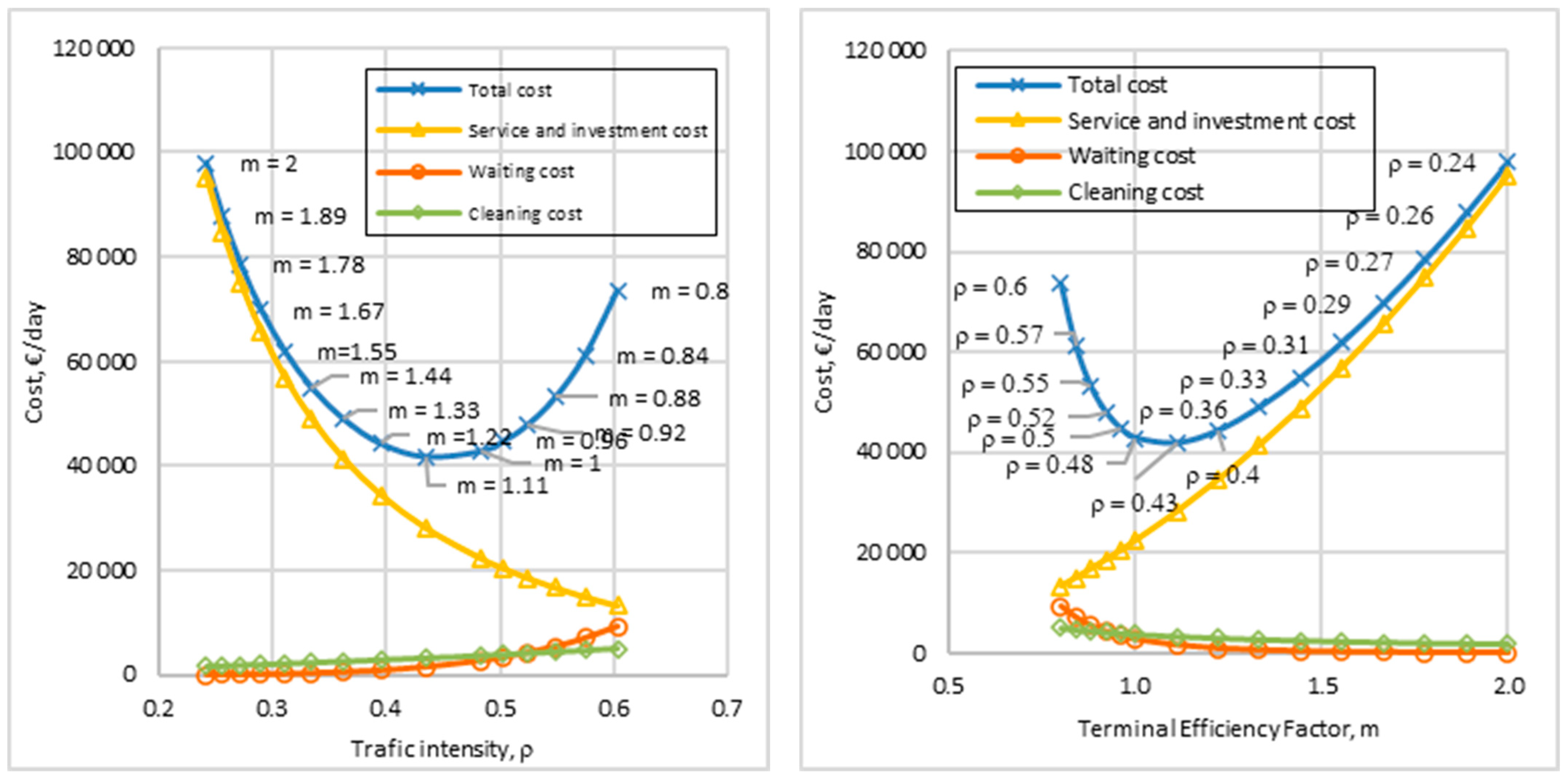
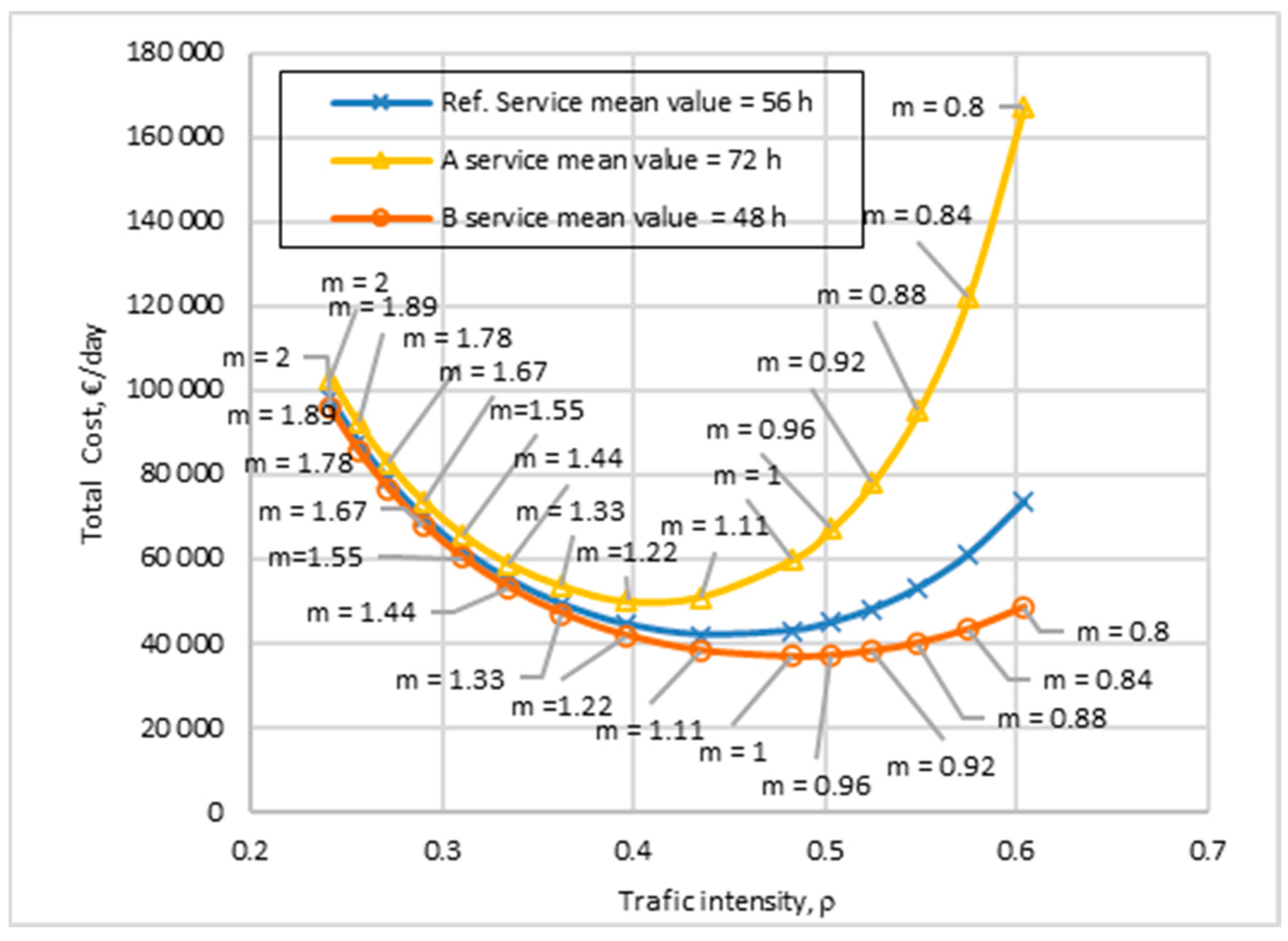
The optimum traffic intensity index
ρ is estimated by minimising the total cost associated with the terminal service and the consequences related to the pollution cleaning. The total cost, cost of berth service, cost of air pollution cleaning, and cost of waiting as a function of the traffic intensity
ρ (
Figure 8 left) and terminal efficiency factor,
m, is shown in
Figure 8, right.
The optimum traffic intensity
) corresponding to a minimum total cost is 0.43, as can be seen from
Figure 8 on the right. The impact of pollution is reflected by increasing the cost associated with air cleaning as the ships are encountered in the port longer. With more intensive traffic, the cost of air pollution increases. Increasing the terminal efficiency reduces the cost associated with air pollution cleaning, but somehow the cost associated with the terminal increases on a different scale.
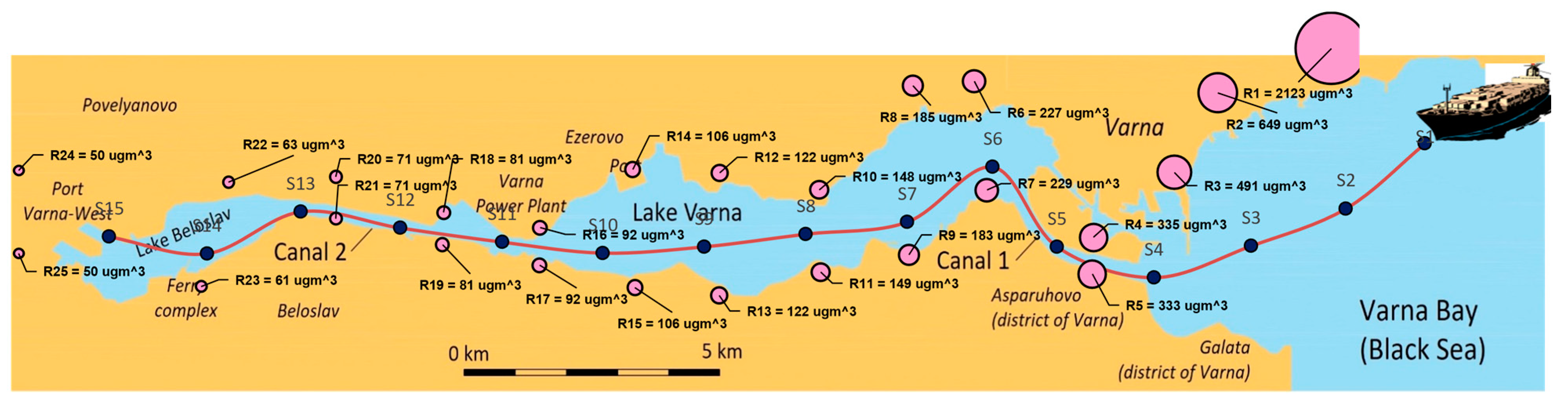
For the ship circulations, conditional on the operational factors and associated cost, the air pollution at different locations along the ships moving from the queuing at the seaport, where several ships are queuing, to the three terminals, where the maximum three ships are processed, is shown in
Figure 9. The rose-scaled circles show the magnitude of the air pollution in μg/m
3. At point
S1, where the ships are queuing, and point
S13, where the terminals are located, the most severe pollution is generated.
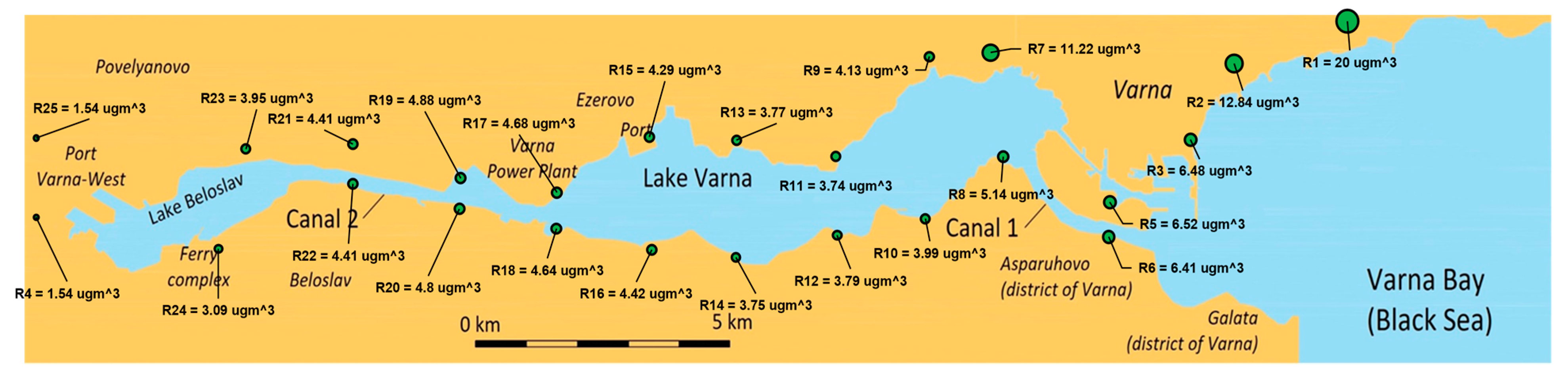
The air pollution concentration after ship emission cleaning, following the maximum acceptable concentration, assumed here as
= 20 μg/m
3, is shown in
Figure 10. The reduction in the air pollution concentration cost is related to 3816 €/day for cleaning all pollutants generated by ships, including
NOx,
SO2, and
PM10. The green-scaled circles show the magnitude of the air pollution in μg/m
3.
The approach developed here is based on the hypothesis that the number of berths is constant. Only the operational factors concerning the terminal operation can be improved to reduce air pollution and associated cost.
Compared to the reference case of an average cargo handling for the three berths of 8808 tonnes/day, the optimal condition for a ship circulating in the port can handle 9777 tonnes/day, and the average time the ship spends in the queue is improved from 2.51 days to 2.18 days. The average number of ships in the queue is changed from 0.2 ship/day to 0.13 ship/day for the optimal solution
The ship waiting cost is reduced from 1563 €/day to 1013 €/day and for cargo waiting cost from 1227 €/day to 796 €/day. The tree berth service and investment costs are 12,000 €/day, and to get the optimal performance, it needs to be increased to 13,320 €/day, and the air pollution cleaning cost is reduced from 3816 €/day to 3374 €/day. The optimal solution will reduce the total cost from 42,911 €/day to 41,874 €/day. It can be concluded that to reduce the total cost by about 4%, the terminal efficiency needs to be improved by 11%, leading to an increase in the service and investment cost.
Figure 11 shows how the total cost changes as a function of the traffic intensity conditional on the service time. For the reference case, which is associated with a service time of 56 h, the optimal traffic intensity is
ρ = 0.43, the optimal terminal efficiency is
m = 1.11, and the total cost is 41,874 €/day. In the case of a service time of 72 h, the optimal traffic intensity is
ρ = 0.47 and the optimal terminal efficiency is
m = 1.22, costing 49,923 €/day. For the case of 48 h of service time, the optimal traffic intensity is 0.42, the optimal terminal efficiency is
m = 1, and the total cost is 36,754 €/day.
8. Conclusions
The present work developed a multidisciplinary approach for evaluating the air pollution and economic impact of ships operating in the port of Varna to identify the most efficient berth terminal operation. The developed approach identified the most efficient berth operation by minimising the cost of implemented ship pollution cleaning measures and overall shipping and terminal operating costs.
The primary contribution of this work is joining well-established methods in a multidisciplinary approach to identify the most efficient terminal operation accounting for air pollution and cost associated with the ship and terminal operations.
Several simplifications in the present study are assumed for the port of Varna. An essential one is that the speed of the ship passing through the canal is assumed to be the maximum allowable speed, according to the canal regulation. Moreover, along the canal, the pilot controls the speed and weather conditions influence it. The study is also based on the hypothesis that the number of berths serving this type of cargo is constant. Only the operational factors concerning the terminals vary and can be improved to reduce air pollution and associated cost.
However, the simplifications are always related to the most conservative scenarios and are not essential for the approach but are needed to demonstrate its capability. Special attention must be paid to the uncertainties involved in the data analysis and the methods involved, which will be part of future studies.
The study demonstrated that the optimal solution would reduce the total cost from 42,911 €/day to 41,874 €/day, which is about 4%. The terminal efficiency needs to be improved by 11%, leading to increased service and investment costs.
The present study is mainly performed for the port of Varna operating conditions, which still is not a part of the emission control areas (ECAs) or sulfur emission control areas (SECAs) that control the pollution generated by ships, and this kind of study is urgently needed for adapting the ship circulation in the port and coastal waters.
As a step further, the developed approach needs to be integrated into a global air pollution quality system, including the air pollution from the city of Varna’s traffic, new ship building and repair yards located in the canal, and any other industrial activity in the vicinity of the port.


