Article

Variability of Equatorial Ionospheric Bubbles over Planetary Scale: Assessment of Terrestrial Drivers

1
GPS Science and Application Research Center, National Central University, Taoyuan 320317, Taiwan
2
Center for Space and Remote Sensing Research, National Central University, Taoyuan 320317, Taiwan
3
Department of Electrical & Electronics Engineering, Birla Institute of Technology & Science-Pilani, K.K. Birla Goa Campus, Sancoale 403726, Goa, India
*
Author to whom correspondence should be addressed.
Atmosphere 2022, 13(9), 1517; https://doi.org/10.3390/atmos13091517
Submission received: 3 August 2022 / Revised: 13 September 2022 / Accepted: 15 September 2022 / Published: 17 September 2022
(This article belongs to the Special Issue Monitoring and Forecasting of Ionospheric Space Weather)

Abstract

:
Nighttime F-region field-aligned irregularities (FAIs) associated with equatorial plasma bubbles (EPBs) are impacted by terrestrial factors, such as solar irradiance and geomagnetic activity. This paper examines the impact of the planetary-scale periodic variability of terrestrial processes on EPB activity. Continual observations of the Equatorial Atmosphere Radar (EAR) have been utilized to derive the intra-seasonal variability of nighttime F-region FAIs in the context of the terrestrial factors mentioned above. A periodicity analysis using wavelet and Lomb–Scargle (LS) spectral analysis indicated significant amplitudes of the long-period planetary-scale variability in the F-region FAI signal-to-noise ratio (SNR), 10.7 cm flux, and geomagnetic indices, as well as a shorter period of variability. Interestingly, a careful inspection of the time series indicated the planetary-scale variability of F-region FAIs to be reasonably out of phase with the periodic geomagnetic variability. EPB occurrence and the FAI signal-to-noise ratio presented a systematic decrease with an increase in the level of geomagnetic activity. Non-transient quiet-time geomagnetic activity has been found to suppress both the occurrence as well as the strength of F-region FAIs. The impacts of planetary-scale geomagnetic activity appear to be non-identical in the summer and equinoctial EPBs. The results highlight the importance of periodic terrestrial processes in driving the planetary-scale variability of EPBs.

1. Introduction

Geomagnetic activity and the controlling space weather processes have been known to influence the energetics and dynamics of the ionosphere–thermosphere system. Over high latitudes, the density and the density irregularities of the ionosphere are not only directly influenced by the particle precipitation following space weather events (e.g., [1]), but also driven by dynamic processes, such as the formation of polar cap patches and polar holes (e.g., [2,3,4]). The ionospheric impact of geomagnetic variability, however, does not remain confined to higher latitudes. The state of the ionosphere over low latitudes is also impacted by the processes associated with geomagnetic activity in various ways (e.g., [5,6,7]). Prompt penetration electric fields can uplift the evening ionosphere, thereby enhancing the growth rate of equatorial Rayleigh-Taylor (RT) instability. Ionospheric disturbance dynamos, which are driven by equatorward wind surges associated with high-latitude joule heating, can also influence night-time low-latitude ionospheric irregularities (e.g., [7,8]). Generally, geomagnetic activity is investigated for its transient influence on low-latitude F-region instability over a time scale of a few tens of minutes to more than a day. However, geomagnetic activity can also impact the low latitude F-region instability on a periodic planetary time scale (e.g., [9]).
The day-to-day variability of equatorial plasma bubbles (EPBs) has been studied over the last several decades because of their detrimental effects on navigation applications. While the solar cycle and seasonal behavior of EPBs are well understood (e.g., [10,11,12]), the prediction of their day-to-day variability continues to be a challenging task for the ionospheric research community (e.g., [13,14,15,16]). EPBs not only display a significant day-to-day variability but they also are impacted by planetary-scale forcing [17,18,19,20,21,22,23,24]. Most of the studies of planetary scale forcing on low latitude ionospheric irregularities have focused on Kelvin and fast Kelvin waves displaying periodicity in the range of 3 to 7 days. However, ionospheric irregularities can also have longer periods of planetary-scale variability [9,25].
Past studies have indicated the periodic variability in RT instability is driven by geomagnetic and related processes [9,26,27]. Modeling investigations have reported the RT instability growth rate to respond to day-to-day changes in geomagnetic activity. Besides the geomagnetic inputs, the generation of ionospheric irregularities can also vary with changes in solar irradiance. In the present study, the intra-seasonal periodic variability of EPBs has been examined in the context of solar irradiance and geomagnetic activity, utilizing the nearly continuous observation of the Equatorial Atmosphere Radar (EAR) in 2012–2013. The study is purely observational, with an emphasis on identifying their relative impact and as importantly, their periodic behavior. While transient processes, such as geomagnetic storms and their impact on ionospheric irregularities, have been extensively investigated, non-transient processes and periodic geomagnetic variability have so far not received as much attention in regards to their impact on ionospheric instability, particularly over low latitudes [17,18]. The results of the study have also been discussed in light of the present understanding of the role of geomagnetic activity in the RT instability process.

2. Equatorial Atmosphere Radar and Related Data Analysis

The Equatorial Atmosphere Radar or EAR is a coherent scatter radar located in Kototabang, Indonesia, and has an operating frequency of 47 MHz. Between 18:00 and 06:00 local time, F-region observations are continuously made using three-beam and 16-beam operations. In the presence of 3 m scale irregularities within radar pulse volume, strong backscattered echoes are detected. EPBs appear as plume structures in EAR observations, as 3 m scale irregularities contained in the EPB, which backscatters the radar energy, traverses over the radar field of view. Fixed beam observations with the EAR, thus, provide a means of examining the dynamics of EPB variabilities. Continuous observation of radar backscattered energy is used to monitor the variability of ionospheric irregularities. Fukao et al. [28] have described the technical details and observational capabilities of the EAR. The present study is based on the fixed beam observation of EPBs during 2012 and 2013 (till ~mid-July). Reasonably continuous observations have been used to examine the intra-seasonal planetary-scale variability of EPBs.
As the field-aligned irregularities (FAIs) associated with EPBs traverse over the radar beam, the imprints of EPBs develop as plume structures in the SNR map (or height–time-intensity map). Figure 1a presents two examples of SNR maps, one recorded on 25 September 2012 and the other on 16 September 2012. On 25 September, plume structures with SNR values as large as 30 dB can be seen in the SNR map, while on 16 September 2012, plume structures are not seen and the SNR remains less than 2 dB (background level). Within an EPB season, EPBs display significant day-to-day variability. To study those variabilities, an F-region SNR from select height bins has been considered. An example is presented in Figure 1b, which shows the SNR recorded by the EAR in the autumnal equinox EPB season in 2012. Here, the top, middle, and bottom panels indicate the SNR of the backscattered echoes from the range bin which is closest to altitudes of 300, 400, and 500 km, respectively. In the figure, the grey color marks the gap in the data. Considering the complexity of operating a large radar system such as the EAR, the data are remarkably continuous. However, one or two days of a continuous data gap can be seen on a few days. Despite these, it is possible to figure out intra-seasonal variabilities in the occurrence of EPBs. For example, the echo SNR is generally higher on day numbers 240–247, 260–280, and 292–305 in comparison to the day numbers sandwiched between them. Thereafter, EPB activity can be seen on day number 325, which was just an isolated occurrence. Possibly, by then the EPB season had ended. EPBs generally display a higher occurrence during equinoctial months due to the alignment of the sunset terminator with the magnetic meridian [29].

3. Results

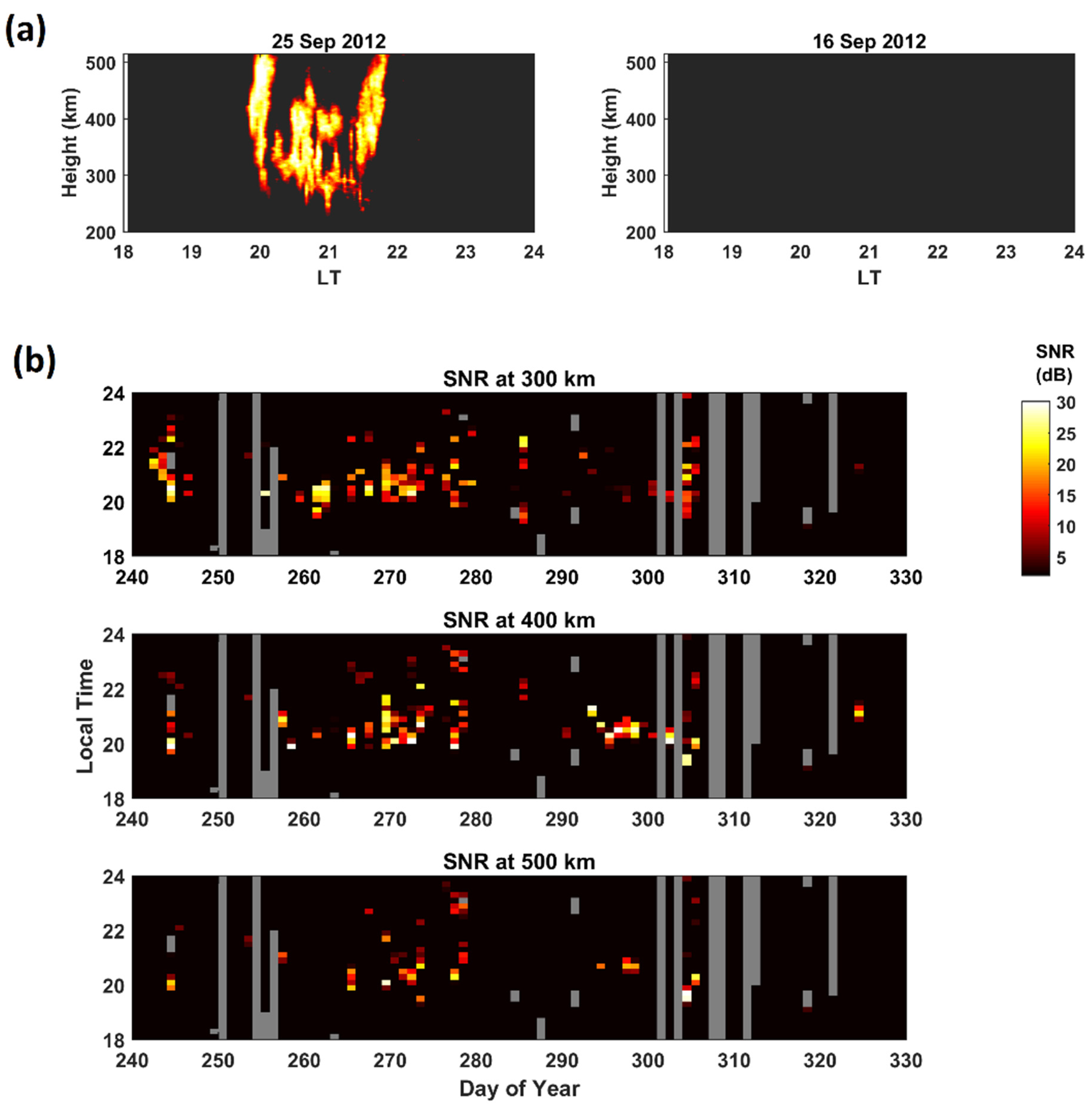
3.1. Intra-Seasonal Variation in Nighttime F-Region Irregularities

Figure 2a presents the day-of-year variation in nocturnal F-region echo SNR from the 300 km height bin. Characteristic seasonal variation can be seen. The onset of EPBs can be seen around the post-sunset period in the equinoctial months and around midnight hours in the summer months. The midnight generation of EPBs in the summer months continues to puzzle researchers. It is widely believed that these are caused by a very sharp vertical electron density gradient in the bottom side of the F-region and the midnight reversal of the zonal electric field [30,31]. While the seasonal variability has already been extensively studied, the intra-seasonal variability of EPBs remains another pertinent topic requiring further studies. Within a season, EPBs display day-to-day and also periodic planetary-scale variations. To study these scales, the day-of-year time series of nocturnal average SNR have been derived for a periodicity analysis. Figure 2b presents the nocturnal average SNR at 300 km. A few days of data gap can be seen sporadically in the series. To perform a wavelet analysis, these gaps are filled using spline interpolation. The interpolated day-of-year series of nocturnal SNR is shown in Figure 2c. The wavelet scalogram that was derived using the day series of average SNR is presented in Figure 2d. A wide range of periods can be seen in that. The interesting aspect is the persistent presence of long-period non-transient variability. Such periods are less likely (though still possible) to be driven by atmospheric planetary-scale activity, for example, Kelvin and fast Kelvin planetary-scale waves. Such periods are generally seen in geomagnetic variables, such as those driven by quasi-27-day solar rotation periodicity. The solar irradiance proxy (f10.7) and geomagnetic variables are also subjected to the wavelet analysis. Figure 2e,f presents the wavelet scalogram of daily F10.7 and the AE index, respectively. These also indicate the very significant presence of long-period non-transient variability.
Another tool for the periodicity analysis of two distinct geophysical time series is the wavelet coherence analysis. The cross wavelet transform of two distinct time series xn and yn can be defined as WXY = WXWY*, in which * denotes the complex conjugate of a series. The cross-wavelet transform results in a complex spectrum. The cross-wavelet power indicates the regions of high common power in the two geophysical series. A vital parameter obtained from the wavelet is coherence, which can be defined as the square of the cross-spectrum normalized by the individual power spectra. Thus, it results in a quantity between zero and one, and can be used as a measure of the cross-correlation between two geophysical time series, but as a function of frequency or time period. A wavelet coherence analysis of the day-of-year series of SNR with f10.7 and the AE index has been carried out to evaluate the extent of coherence in these quantities. The wavelet coherence analysis of the day-of-year series of SNR with f10.7 and an AE index is presented in Figure 3. Panels (a) and (b) present the wavelet coherence of SNR with F10.7 and the AE index, respectively. Magnitude-squared wavelet coherence is a measure of the correlation between the two parameters in the time-frequency (period) plane. In this analysis, the SNR shows significant coherence with the two parameters. Of particular interest is the remarkable coherence seen between SNR and AE in the autumnal equinox months in 2012.

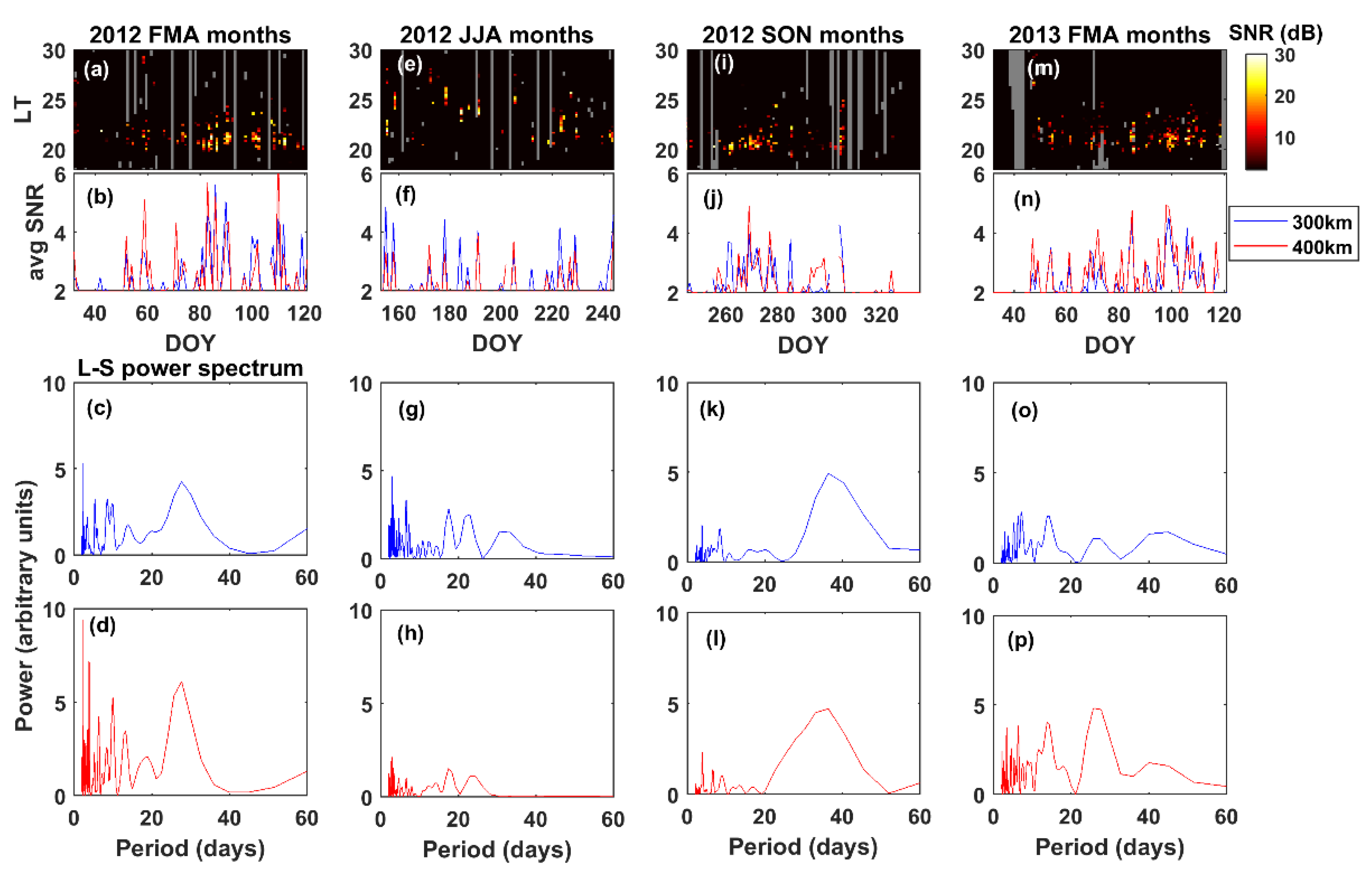
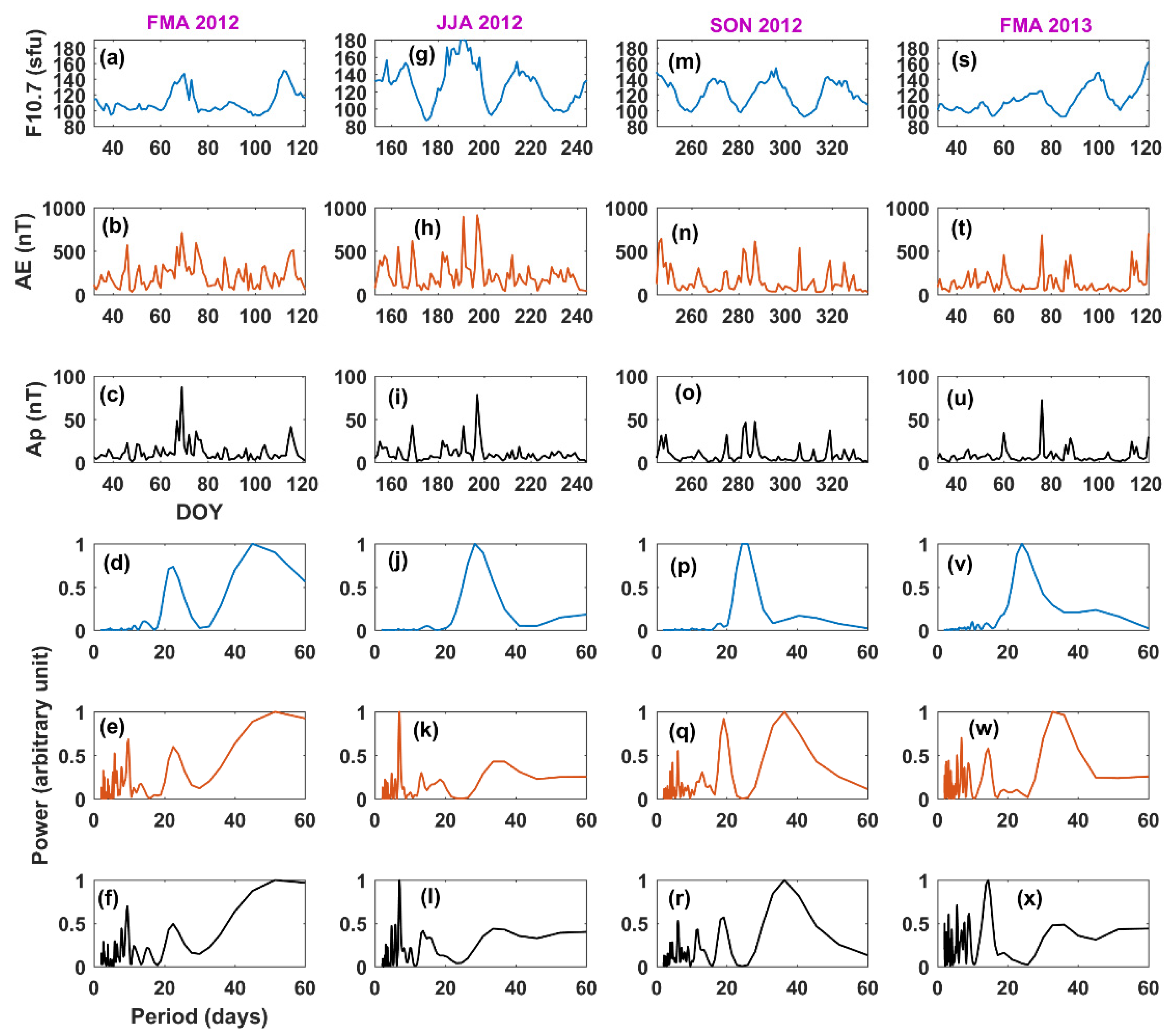
3.2. Intra-Seasonal Periodicities in Equinox and Summer Months

Figure 4 presents the F-region SNR variation in the equinox (Vernal: Febuary, March, April, and Autumnal: September, October, November) and summer (June, July, August) months. The top row (panels a, e, i, and m) shows SNR variation at the height of 300 km. The row below (panels b, f, j, and n) shows nocturnal average SNR at 300 km (blue) and 400 km (red) in different seasons. The last two rows present corresponding Lomb–Scargle (LS) power spectra calculated using the day series of the nocturnal average SNR at 300 km and 400 km, respectively, in different seasons arranged column-wise. The L–S spectrum, which is based on a sinusoidal fit on the time series, provides an efficient method of deriving periodicities. It can be effectively used to derive periodicity information, even if the time series is not larger than the period of interest. The L–S technique offers better frequency resolution than the FFT and can be effectively utilized in the areas in which the exact period is required to be extracted from a time series not significantly longer than the period of interest [9,32]. The L–S technique can even be used when gaps exist in the data or when the sampling is not periodic (unlike FFT, in which periodic sampling is required). The L–S spectra presented in Figure 4 indicate the prevalence of planetary-scale periodicities in all seasons. Spectral peaks greater than a 20-day period are identifiable and the shapes of the spectra are similar at both height levels.
The F10.7 and geomagnetic variations with their corresponding L–S spectra in equinox (Vernal: Febuary, March, April, and Autumnal: September, October, November) and summer (June, July, August) months are shown in Figure 5. Panels indicating seasons are arranged column-wise, and row-wise they indicate different indices and the corresponding L–S spectra. The top three rows present f10.7, AE, and Ap indices, respectively, in different months. The bottom three rows present their corresponding L–S spectra, respectively. Planetary-scale variations can be seen in these parameters and their periodicity has a reasonable resemblance to those of the SNR shown in Figure 4, though not identical in every case.
Having examined the spectra of the concerned parameters, it may be important to examine the day series, piece-wise. Thus, the day series of SNR, AE, and F10.7 is visually examined for each season. Figure 6 presents the day series of nocturnal average SNR at 300 km, the AE index, and f10.7 in the equinoctial and summer months. Figure 6a–d shows these parameters for each set of months (Vernal Equinox: Febuary, March, April; Summer: June, July, August; and Autumnal Equinox: September, October, November). In each of these panels, the nocturnal average SNR (300 km), AE index, and F10.7 are presented in the top, middle, and bottom sub-panels, respectively. A distinct relation may not appear from such comparisons; however, some broad features can be seen. For example, in panel (a), the clusters of high-SNR days can generally be seen as having a lesser value of the AE index. In panel (a), the SNR is generally low (high) during the 60–80th (80–100th) days of the year in 2012, while the pattern of the AE index is the opposite. Such variability may have different scales. Additionally, in the summer months (June, July, and August) shown in Panel (b), the high-SNR cases are not clustered, but rather sporadic. Any periodic comparison between the SNR and the geomagnetic variability may not match one-to-one, because there is also an inherent or day-to-day variability of EPBs, which may not be driven by geomagnetic activity.

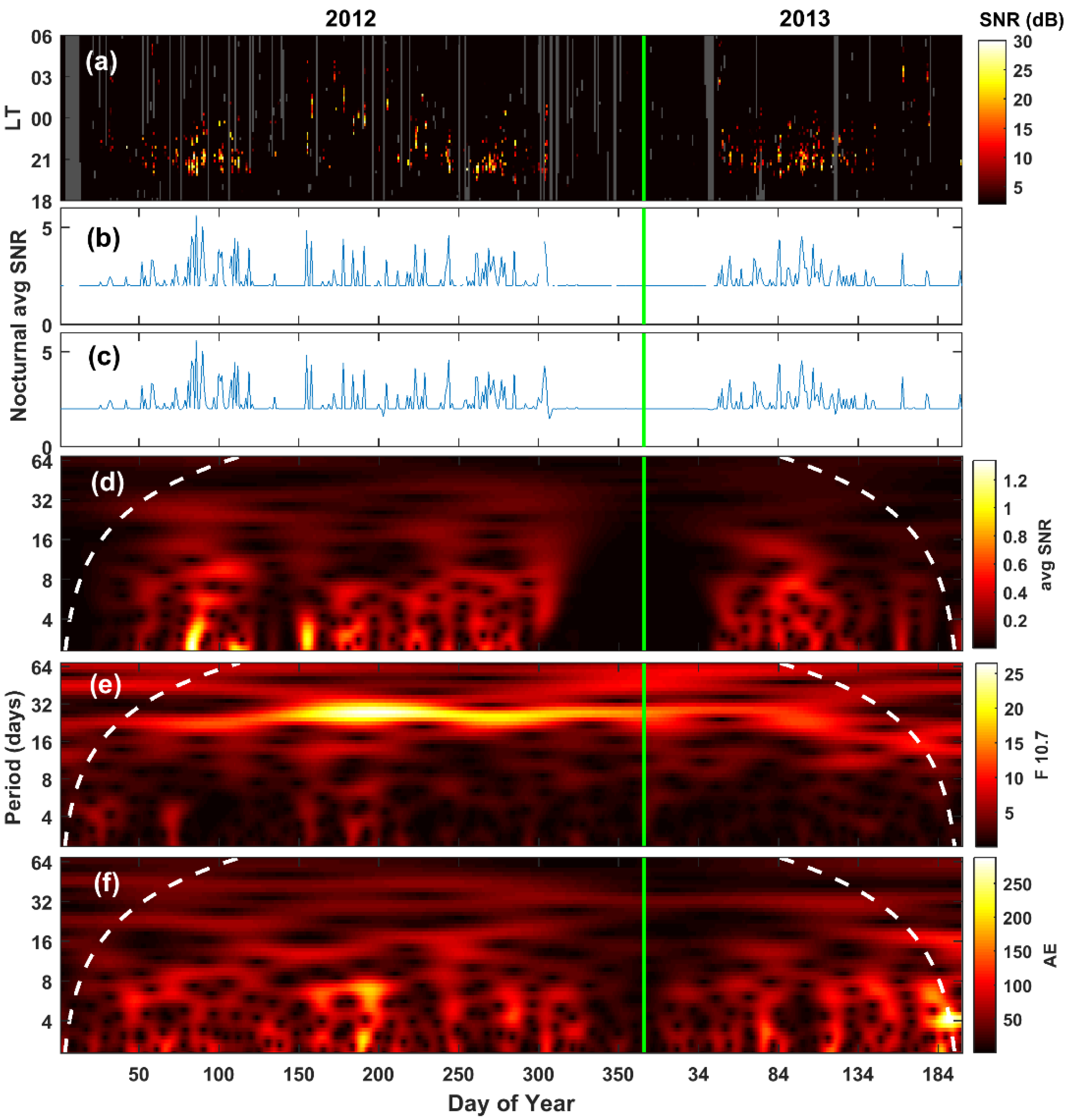
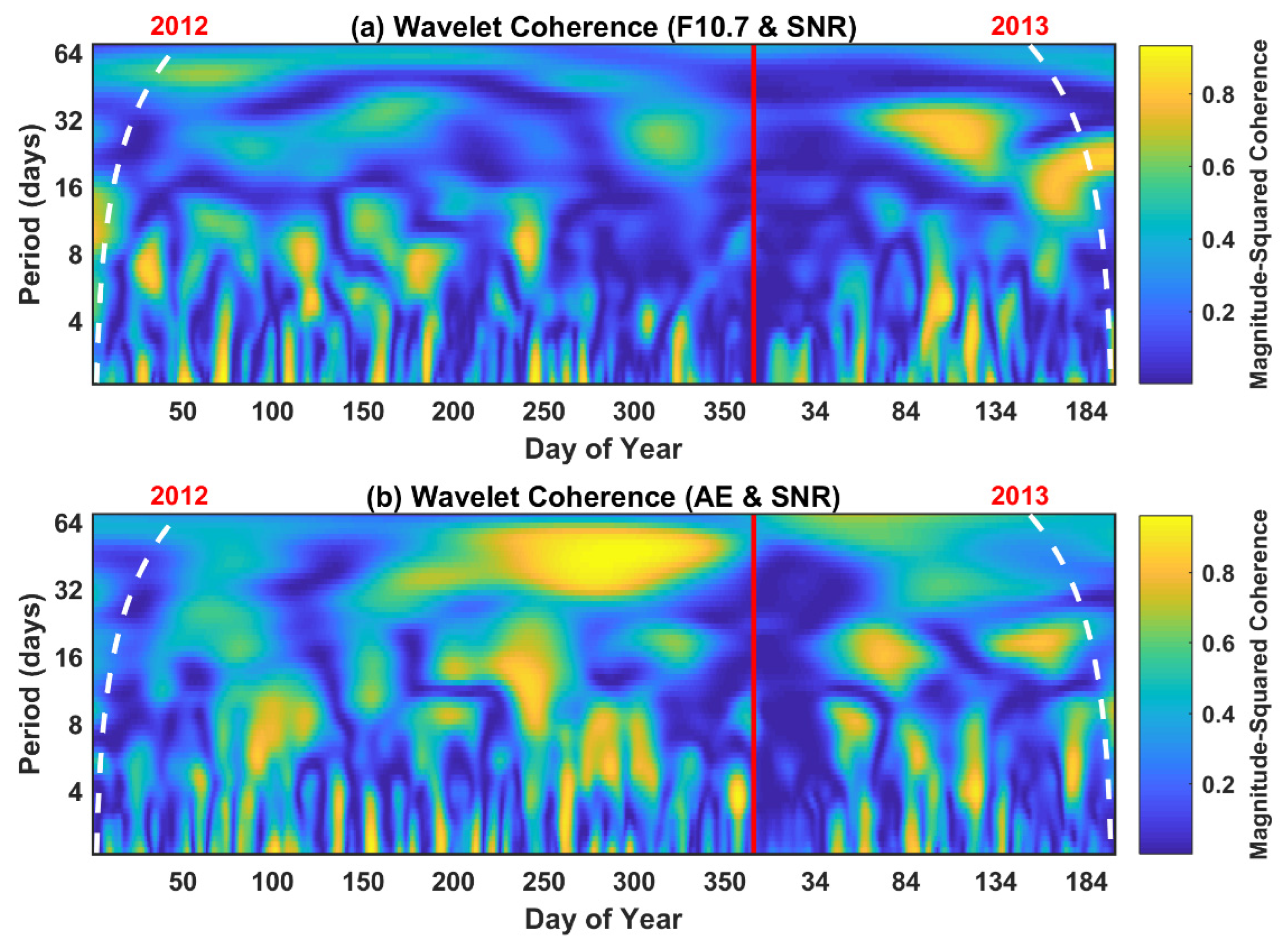
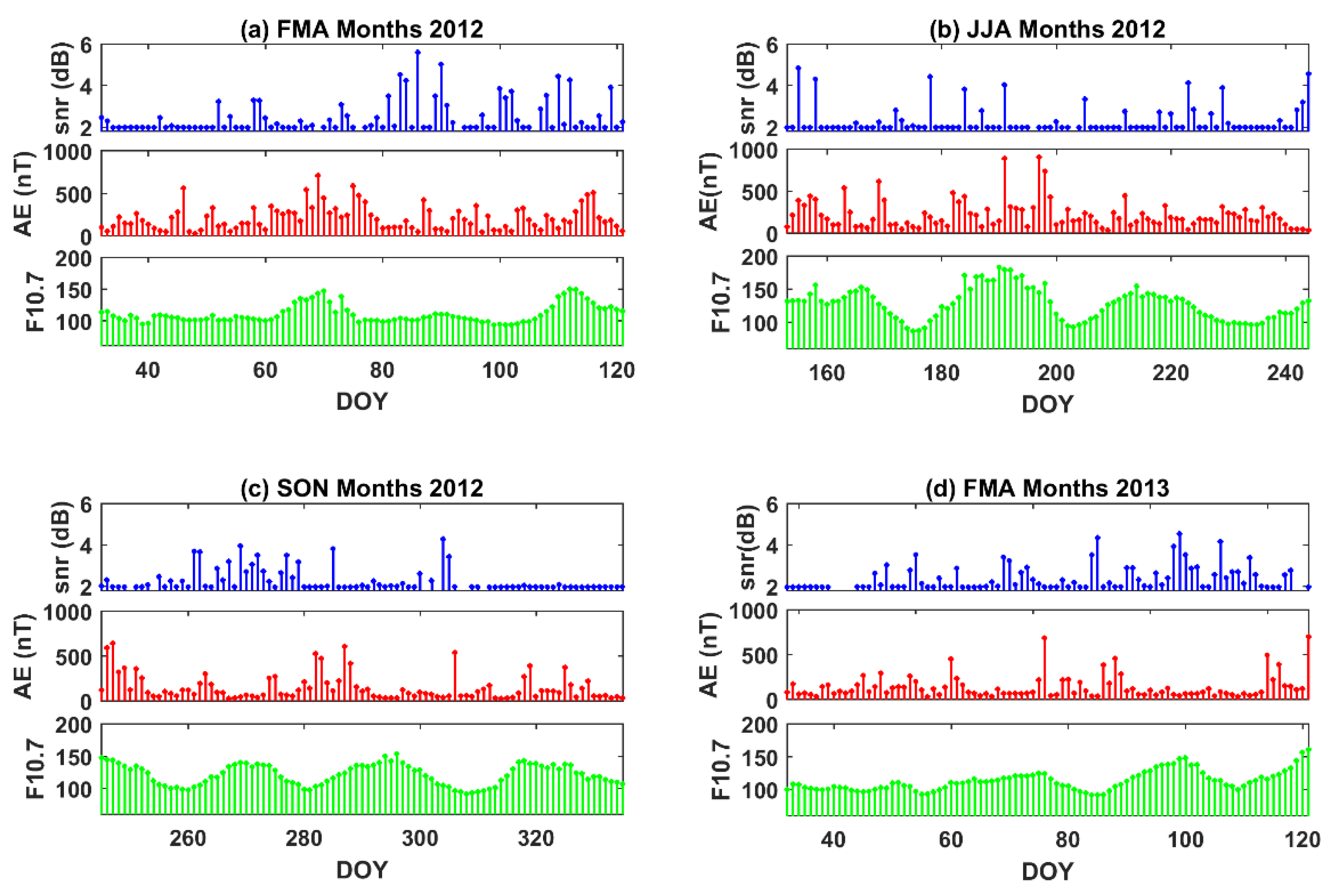
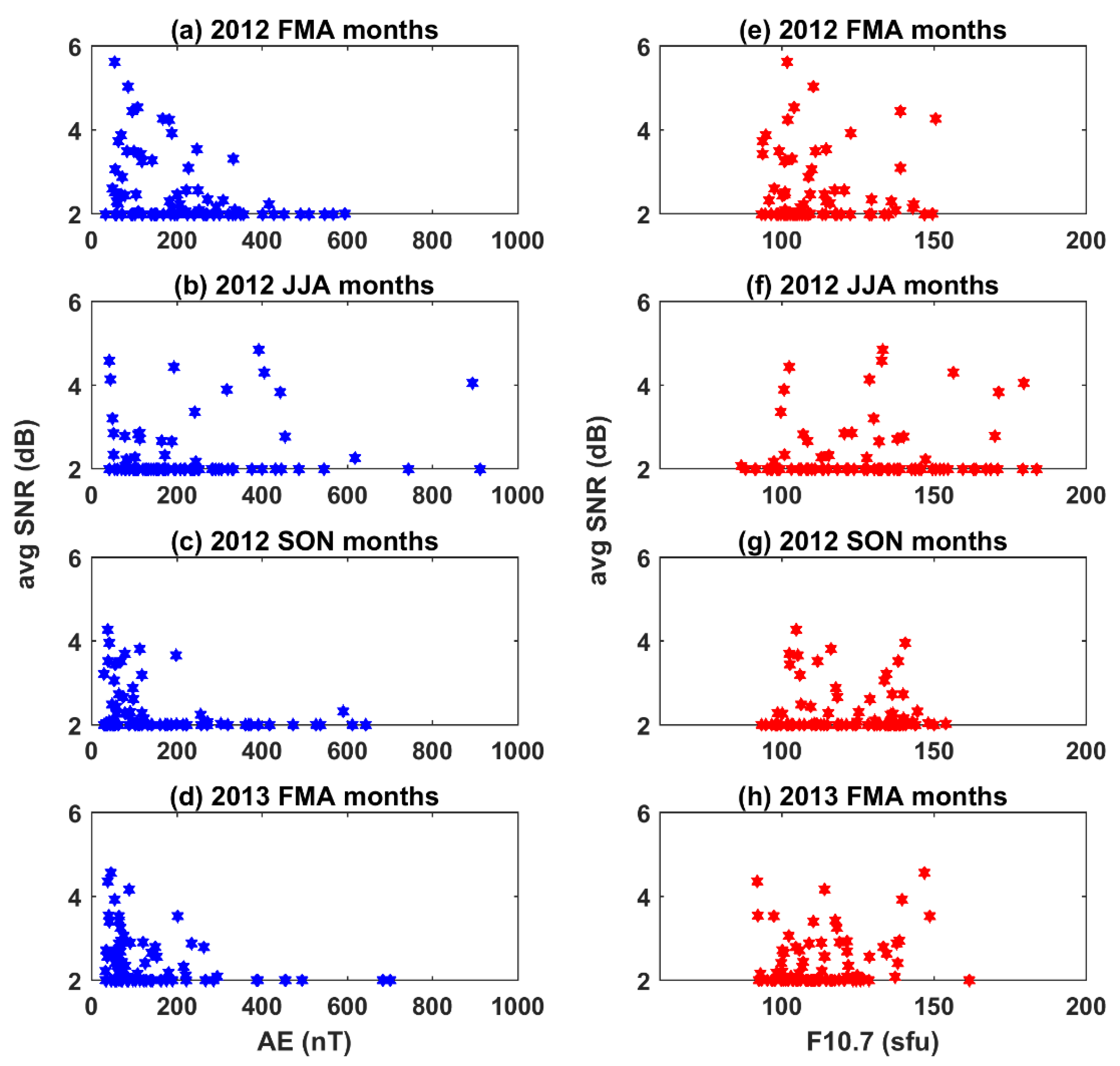
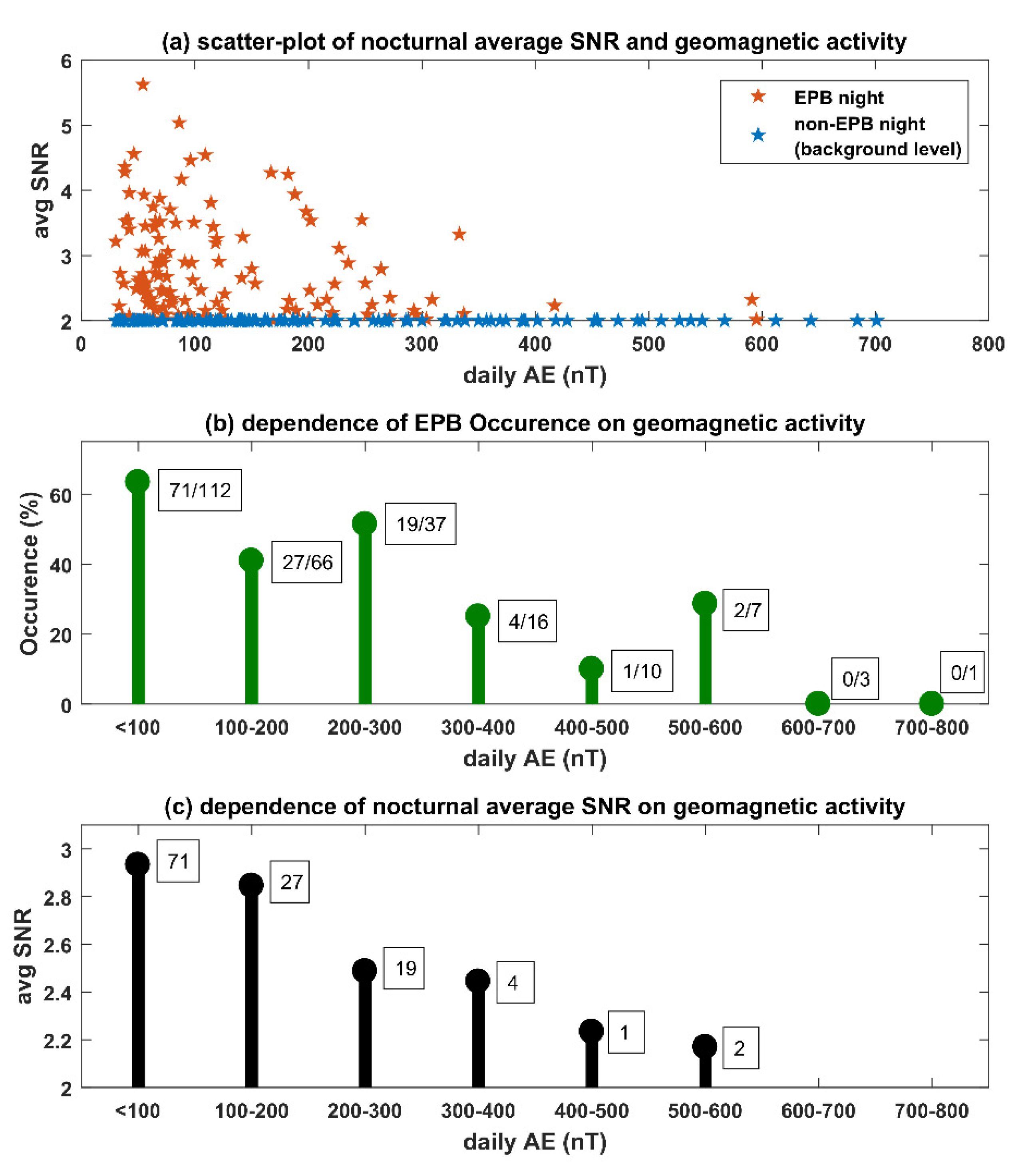
3.3. Relation of SNR with AE Index and F10.7 in Different Seasons

To evaluate the relation of nocturnal average SNR driven by geomagnetic and solar irradiance variability, a scatter plot analysis has been performed. In that, the nocturnal average SNR (300 km) is plotted on the y-axis and the geomagnetic/irradiance proxy parameter is plotted on the x-axis. Figure 7a–d presents a scatter analysis of the nocturnal average SNR with the AE index in the equinox (vernal and autumnal) and summer months. Figure 7e–h presents the same, but for the nocturnal average SNR with F10.7. This analysis shows that (a) in the equinox months, geomagnetic quiet days had higher nocturnal SNR; (b) in the summer months, the geomagnetic activity did not display any systematic relation to nocturnal SNR; and, (c) that it is hard to figure out any systematic relation of F10.7 to nocturnal average SNR.
The relation between nocturnal SNR and AE index, in all the equinoctial months (Febuary–April and September–November) combined, is further evaluated from the perspective of EPB occurrence and nocturnal average SNR during EPB nights. Figure 8a shows the scatter plot of nocturnal SNR at 300 km with the AE index in all the equinox seasons combined. Here, the orange (blue) color indicates EPB (non-EPB) nights. Besides having higher SNR (higher than background level), EPB nights have also been verified by carefully examining the Height–Time–SNR map of individual nights. The nocturnal SNR indicates an inverse relation with geomagnetic activity. Figure 8b presents a bar plot of the EPB occurrence in piece-wise incremental geomagnetic activity in terms of the AE index, with 100 nT steps. For calculating the occurrence in each step, the number of EPB nights is divided by the total number of nights (EPB and non-EPB) and then multiplied by 100 to obtain the percentage. The EPB occurrence is >60% for the AE < 100. In Figure 8b, the box adjacent to each stem indicates the number of EPB cases/total cases for that particular AE step. The number of cases in each AE step is not the same and decreases with the level of AE. The largest number of observations corresponds to an AE indices less than 100. Occurrence, however, shows a trend. In general, the occurrence shows a systematic decrease with an increase in the value of the AE index. Figure 8c presents the bar plot of nocturnal average SNR at 300 km (of the EPB cases only) in piece-wise incremental geomagnetic activity in terms of the AE index, with 100 nT steps. The box adjacent to each stem indicates the number of EPB cases for that particular AE step. It may be noted that only the EPB nights have been considered when calculating the nocturnal average SNR for each AE index step. A clear decrease in nocturnal SNR can be seen with an increase in the value of the AE index. This shows that geomagnetic activity not only influences the occurrence of EPBs, but also that of the echo SNR. A higher nocturnal SNR may indicate the presence of strong plasma irregularities.

4. Discussion

The variability of equatorial F-region irregularities and their time scales have been a long-standing subject of investigation. The prediction of EPBs, which are considered detrimental for satellite-based navigation/communication, continues to remain a challenging task for the research community. Of particular interest has been the planetary-scale variability of EPBs [17,18,19,20,21,22,23,24]. A deeper understanding of the planetary-scale variability can contribute significantly to the development of the EPB prediction model. Such an information can be utilized to separate contiguous clusters of days that have a higher probability of EPB occurrence from those with a lower probability, thus facilitating extended range prediction. For that, knowledge of the prevailing periodicities of planetary-scale waves becomes a prerequisite. A wide spectrum of planetary-scale variabilities of EPBs has been reported with periods in the ranges of 4–8 days, 10–15 days, and more. Most of the investigations have, however, focused on 4–8 day waves which are considered to be due to the Kelvin and fast Kelvin waves that originate in the lower atmosphere. Such scales can also be seen in the EAR observations presented in this study. In the present investigation, however, the F-region SNR indicates the significant presence of long-period planetary-scale variability. Past investigations have reported planetary-scale variability of equatorial ionospheric irregularities driven by geomagnetic activity [9,26,27]. The interesting aspect of this investigation is that the variability of EPBs and geomagnetic activity are out of phase. The present results seem to suggest that the periodic geomagnetic activity has caused the planetary-scale variability of EPBs by suppressing the generation of EPBs. EPBs displayed a much higher occurrence on days with AE indices < 300 nT in comparison to higher levels of AE indices. For the characterization of the role of geomagnetic activity in suppressing the generation of EPBs, the AE index has been regarded as a measure of geomagnetic activity (Figure 8). While the periodic observation is also consistent in other geomagnetic indices, the AE index represents an amplified version of geomagnetic activity with a higher range of the magnitude of variability. The AE index is derived from observations in the auroral electrojet region, where energy deposition due to Joule heating takes place. This might also highlight possible thermospheric heating associated with the periodic variability of geomagnetic activity, even though the observations are consistent with other indices (except for the Dst index, representing the ring current variability, which does not highlight planetary-scale processes, such as quasi-27-day solar rotation).
The role of high-latitude magnetic activity on transient (relatively short term in comparison to planetary time scale) low-latitude processes has already been extensively studied. For example, the roles of the prompt penetration electric field (PPEF) and the ionospheric disturbance dynamo on equatorial RT instability are already known. The PPEF influences the equatorial processes over a time scale of a few minutes to more than an hour, while the disturbance dynamo influences the low-latitude processes over a time scale of a few hours to more than a day. Enhanced energy deposition due to geomagnetic activity can also modify thermospheric energetics, thereby impacting the ion-neutral collision and composition. Going beyond the purview of transient geomagnetic events, the planetary-scale variability of geomagnetic activity can also impact low-latitude ionospheric irregularities. Because the two are out of phase, it suggests that the non-transient enhancement in geomagnetic activity suppresses the genesis of EPBs. One possible explanation is related to the enhancement of the ion-neutral collision frequency in the ionosphere-thermosphere system, driven by enhanced geomagnetic activity which in turn impacts the RT instability over a planetary scale. While it just remains a hypothesis, this requires further investigation.
The planetary-scale variability of equatorial ionospheric irregularities in the context of geomagnetic activity has been studied by Carter et al. [33]. Based on TIEGCM model simulations, they reported that the geomagnetic activity causes an enhancement of high-latitude joule heating, which results in the suppression of the low-latitude F-region dynamo and subsequently the F-layer uplift. A recent report based on continuous measurements of ionospheric irregularities using Jicamarca radar has also indicated a close relationship between the ionospheric irregularities and the auroral electrojet [34]. The relationship was not limited to transient geomagnetic processes and displayed periodic behavior. In the present investigation, the time series of the daily averaged values of the geomagnetic parameters and their spectra indicates that space weather conditions can be quite periodic in nature. Such periodic geomagnetic activity may induce the large-scale variability in the ionosphere–thermosphere system over low latitudes. The AE index is considered proportional to the Joule heating in high latitudes [35]. High-latitude joule heating can influence ionospheric processes in several ways. Disturbance dynamos that are associated with the high-latitude Joule heating during intense space weather events such as geomagnetic storms usually have time scales of 4 to 30 h. Another outcome associated with high-latitude Joule heating is large-scale traveling ionospheric disturbances (LSTIDs). Going beyond the purview of intense space weather events, the planetary-scale variability of the auroral electrojet can possibly create a similar variability in high latitude Joule heating. This in turn can affect the background thermospheric/ionospheric circulation and composition over a similar time scale, influencing the low-latitude ionospheric instability processes. In this hypothesis, low-latitude variability is only an effect, the cause of which is planetary-scale geomagnetic forcing.
As presented in the scatter-plot analysis, the nocturnal average SNR displayed a systematic relation with the AE index in the equinoctial months. However, the SNR during the summer months did not show any systematic relation with the AE or F10.7. This seems to indicate that the summer-time irregularities are not impacted by periodic planetary-scale variations in geomagnetic activity as they are in the equinoctial period. Unlike in the equinoctial months, the summer-time EPBs are generated during the midnight hours (e.g., [30,31]). The causative mechanism of summer-time EPBs is quite different from that in the equinoctial period [36]. Summer-time EPBs are generally considered to be driven by the midnight reversal of the zonal electric field, causing an upliftment of the F layer. This, together with a very sharp vertical gradient in the F-layer bottom-side electron density during the midnight hours, enhances the growth rate of the RT instability [31]. Unlike in the equinoctial months, when the enhancement in geomagnetism results in the suppression of the F-region dynamo [33], in the summer months the vertical uplift of the F layer in the midnight hours may have different drivers. A recent investigation has suggested that the midnight reversal of the zonal electric field that uplifts the F layer can actually be driven by migrating semidiurnal tides [37]. Thus, the mechanism for the post-sunset uplift of the F layer in equinoctial months is totally non-identical to that for the midnight uplift during summer months. Therefore, the periodic planetary-scale variation in geomagnetic activity may have a non-identical impact on the EPBs in the summer and equinoctial periods. The relation of SNR with F10.7 did not display any systematic behavior, unlike with geomagnetic activity. F10.7 is considered to be a proxy for solar ionizing radiation, which can drive changes in the background ionization. It remains somewhat unclear as to why the periodic planetary-scale variation in F10.7 did not drive a systematic variation in the F-region SNR.
The Lomb–Scargle analysis has been utilized to understand the prevailing periodicity in equinoctial and summer months. The geomagnetic activity and SNR variability indicated a broadly similar range. The exact periods of the two may not match in the LS spectra, as the EPBs will also have their intrinsic variability, which may influence the periodicity. The broad relationship, however, suggests that geomagnetic activity has a significant impact on the planetary-scale variability of the EPBs. The variability of the EPBs can manifest in terms of both its occurrence and the average SNR. Figure 8b,c suggests that geomagnetic activity influences both of these aspects. The occurrence of EPBs relates to the presence of field-aligned irregularities, while the nocturnal average SNR refers to the strength of field-aligned irregularities.

5. Summary

The vital aspects of the present investigation may be summarized as follows:
(a) Nocturnal F-region irregularities in EAR observations have indicated the presence of strong planetary-scale variability. (b) The geomagnetic AE index and F10.7 also presented long-period planetary-scale variabilities in them. (c) The planetary-scale variability of ionospheric irregularity was out of phase with respect to geomagnetic activity. (d) Careful analysis suggested that the role of geomagnetic activity in driving the variability of ionospheric irregularity was predominantly linked with the suppression of RT instability. (e) Geomagnetic activity not only influences the occurrence of EPBs but also the strength of the irregularities as determined by the nocturnal average SNR. The present study highlights that an EPB prediction scheme must take into account the planetary-scale variability of EPBs and their driving mechanisms.

Author Contributions

Conceptualization, L.M.J., L.-C.T. and S.-Y.S.; methodology, L.M.J. and L.-C.T.; validation, L.M.J., L.-C.T. and S.-Y.S.; investigation, L.M.J. and L.-C.T.; resources, L.M.J. and L.-C.T.; visualization, L.M.J. and A.D.; project administration, L.M.J.; funding acquisition, L.M.J. All authors have read and agreed to the published version of the manuscript.

Funding

This work is supported by the Ministry of Science and Technology (MOST) of Taiwan. Funding grant number MOST-110-2111-M-008 -006 -MY3.

Institutional Review Board Statement

Not applicable.

Informed Consent Statement

Not applicable.

Data Availability Statement

EAR data used in this paper (2012–2013) can be accessed from the EAR data repository (http://www.rish.kyoto-u.ac.jp/ear/index-e.html, accessed on 12 September 2022). The analyzed datasets generated for this study are available on request from the lead author.

Acknowledgments

EAR data are provided by the Research Institute for Sustainable Humanosphere of Kyoto University. EAR data used in this paper (2012–2013) can be accessed from the EAR data repository (http://www.rish.kyoto-u.ac.jp/ear/index-e.html, accessed on 12 September 2022). Geomagnetic and F10.7 cm flux data used in the study (2012–2013) were downloaded from the Omni web data repository (https://omniweb.gsfc.nasa.gov/form/dx1.html, accessed on 12 September 2022).

Conflicts of Interest

The authors declare no conflict of interest.

References

  1. Jin, Y.; Spicher, A.; Xiong, C.; Clausen, L.B.N.; Kervalishvili, G.; Stolle, C.; Miloch, W.J. Ionospheric plasma irregularities characterized by the Swarm satellites: Statistics at high latitudes. J. Geophys. Res. Space Phys. 2019, 124, 1262–1282. [Google Scholar] [CrossRef]
  2. Crowley, G.; Carlson, H.C.; Basu, S.; Denig, W.F.; Buchau, J.; Reinisch, B.W. The dynamic ionospheric polar hole. Radio Sci. 1993, 28, 401–413. [Google Scholar] [CrossRef]
  3. Oksavik, K.; Barth, V.L.; Moen, J.; Lester, M. On the entry and transit of high-density plasma across the polar cap. J. Geophys. Res. 2010, 115, A12308. [Google Scholar] [CrossRef]
  4. Lamarche, L.J.; Makarevich, R.A. Radar observations of density gradients, electric fields, and plasma irregularities near polar cap patches in the context of the gradient-drift instability. J. Geophys. Res. Space Phys. 2017, 122, 3721–3736. [Google Scholar] [CrossRef]
  5. Abdu, M.A.; Batista, I.S.; Bertoni, F.; Reinisch, B.W.; Kherani, E.A.; Sobral, J.H.A. Equatorial ionosphere responses to two magnetic storms of moderate intensity from conjugate point observations in Brazil. J. Geophys. Res. 2012, 117, A05321. [Google Scholar] [CrossRef]
  6. Joshi, L.M.; Sripathi, S.; Singh, R. Simulation of low-latitude ionospheric response to 2015 St. Patrick's Day super geomagnetic storm using ionosonde-derived PRE vertical drifts over Indian region. J. Geophys. Res. Space Phys. 2016, 121, 2489–2502. [Google Scholar] [CrossRef]
  7. Kakad, B.; Surve, G.; Tiwari, P.; Yadav, V.; Bhattacharyya, A. Disturbance dynamo effects over low-latitude F region: A study by network of VHF spaced receivers. J. Geophys. Res. Space Phys. 2017, 122, 5670–5686. [Google Scholar] [CrossRef]
  8. Blanc, M.; Richmond, A. The ionospheric disturbance dynamo. J. Geophys. Res. 1980, 85, 1669–1686. [Google Scholar] [CrossRef]
  9. Joshi, L.M.; Tsai, L.-C.; Su, S.-Y.; Caton, R.G.; Groves, K.M.; Lu, C.-H. On the nature of the intraseasonal variability of nighttime ionospheric irregularities over Taiwan. J. Geophys. Res. Space Phys. 2019, 124, 3609–3622. [Google Scholar] [CrossRef]
  10. Nishioka, M.; Saito, A.; Tsugawa, T. Occurrence characteristics of plasma bubble derived from global ground-based GPS receiver networks. J. Geophys. Res. 2008, 113, A05301. [Google Scholar] [CrossRef]
  11. Joshi, L.M.; Patra, A.K.; Rao, S.V.B. Equatorial F-region irregularities during low and high solar activity conditions. Indian J. Radio Space Phys. 2012, 41, 208–219. [Google Scholar]
  12. Smith, J.; Heelis, R.A. Equatorial plasma bubbles: Variations of occurrence and spatial scale in local time, longitude, season, and solar activity. J. Geophys. Res. Space Phys. 2017, 122, 5743–5755. [Google Scholar] [CrossRef]
  13. Tsunoda, R.T. Satellite traces: An ionogram signature for large-scale wave structure and a precursor for equatorial spread F. Geophys. Res. Lett. 2008, 35, L20110. [Google Scholar] [CrossRef]
  14. Hysell, D.L.; Chun, J.; Chau, J.L. Bottom-type scattering layers and equatorial spread F. Ann. Geophys. 2004, 22, 4061–4069. [Google Scholar] [CrossRef]
  15. Joshi, L.M. LSWS linked with the low-latitude Es and its implications for the growth of the R-T instability. J. Geophys. Res. Space Phys. 2016, 121, 6986–7000. [Google Scholar] [CrossRef]
  16. Nugent, L.D.; Elvidge, S.; Angling, M.J. Comparison of low-latitude ionospheric scintillation forecasting techniques using a physics-based model. Space Weather 2021, 19, e2020SW002462. [Google Scholar] [CrossRef]
  17. Abdu, M.A.; Ramkumar, T.K.; Batista, I.S.; Brum, C.G.M.; Takahashi, H.; Reinisch, B.W.; Sobral, J.H.A. Planetary wave signatures in the equatorial atmosphere–ionosphere system, and mesosphere- E- and F region coupling. J. Atmos. Sol.-Terr. Phys. 2006, 68, 509–522. [Google Scholar] [CrossRef]
  18. Abdu, M.A.; Brum, C.G.M. Electrodynamics of the vertical coupling processes in the atmosphere–ionosphere system of the low latitude region. Earth Planets Space 2009, 61, 385–395. [Google Scholar] [CrossRef]
  19. Bertoni, F.C.P.; Sahai, Y.; Raulin, J.P.; Fagundes, P.R.; Pillat, R.V.G.; Gimenez deCastro, C.G.W.; Lima, L.C. Equatorial spread-F occurrence observed at two near equatorial stations in the Brazilian sector and its occurrence modulated byplanetary waves. J. Atmos. Sol.-Terr. Phys. 2011, 73, 457–463. [Google Scholar] [CrossRef]
  20. Fagundes, P.R.; Bittencourt, J.A.; Abalde, J.R.; Sahai, Y.; Bolzan, M.J.A.; Pillat, V.G.; Lima, W.L.C. F layer postsunset height rise due to electric field prereversal enhancement: 1. Traveling planetary wave ionospheric disturbance effects. J. Geophys. Res. Space Phys. 2009, 114, A12321. [Google Scholar] [CrossRef]
  21. Takahashi, H.; Wrasse, C.M.; Pancheva, D.; Abdu, M.A.; Batista, I.S.; Lima, L.M.; Batista, P.P.; Clemesha, B.R.; Shiokawa, K. Signatures of 3–6 day planetary waves in the equatorial mesosphere and ionosphere. Ann. Geophys. 2006, 24, 3343–3350. [Google Scholar] [CrossRef] [Green Version]
  22. Takahashi, H.; Abdu, M.A.; Wrasse, C.M.; Fechine, J.; Batista, I.S.; Pancheva, D.; Lima, L.M.; Batista, P.P.; Clemesha, B.R.; Shiokawa, K.; et al. Possible influence of ultra-fast Kelvin wave on the equatorial ionosphere evening uplifting. Earth Planets Space 2009, 61, 455–462. [Google Scholar] [CrossRef]
  23. Liu, G.; Immel, T.J.; England, S.L.; Frey, H.U.; Mende, S.B.; Kumar, K.K.; Ramkumar, G. Impacts of atmospheric ultrafast Kelvin waves on radio scintillations in the equatorial ionosphere. J. Geophys. Res. Space Phys. 2013, 118, 885–891. [Google Scholar] [CrossRef]
  24. de Abreu, A.J.; Fagundes, P.R.; Bolzan, M.J.A.; de Jesus, R.; Pillat, V.G.; Abalde, J.R.; Lima, W.L.C. The role of the traveling planetary wave ionospheric disturbances on the equatorial F region post-sunset height rise during the last extreme low solar activity and comparison with high solar activity. J. Atmos. Sol.-Terr. Phys. 2014, 113, 47–57. [Google Scholar] [CrossRef]
  25. Ogawa, T.; Miyoshi, Y.; Otsuka, Y.; Nakamura, T.; Shiokawa, K. Equatorial GPS ionospheric scintillations over Kototabang, Indonesia and their relation to atmospheric waves from below. Earth Planets Space 2009, 61, 397–410. [Google Scholar] [CrossRef]
  26. Carter, B.A.; Retterer, J.M.; Yizengaw, E.; Groves, K.; Caton, R.; McNamara, L.; Bridgwood, C.; Francis, M.; Terkildsen, M.; Norman, R.; et al. Geomagnetic control of equatorial plasma bubble activity modeled by the TIEGCM with Kp. Geophys. Res. Lett. 2014, 41, 5331–5339. [Google Scholar] [CrossRef]
  27. Shinagawa, H.; Jin, H.; Miyoshi, Y.; Fujiwara, H.; Yokoyama, T.; Otsuka, Y. Daily and seasonal variations in the linear growth rate of the Rayleigh-Taylor instability in the ionosphere obtained with GAIA. Prog. Earth Planet. Sci. 2018, 5, 16. [Google Scholar] [CrossRef]
  28. Fukao, S.; Hashiguchi, H.; Yamamoto, M.; Tsuda, T.; Nakamura, T.; Yamamoto, M.K.; Sato, T.; Hagio, M.; Yabugaki, Y. Equatorial Atmosphere Radar (EAR): System description and first results. Radio Sci. 2003, 38, 1053. [Google Scholar] [CrossRef]
  29. Tsunoda, R.T. Control of the seasonal and longitudinal occurrence of equatorial scintillations by the longitudinal gradient in integrated E region Pedersen conductivity. J. Geophys. Res. 1985, 90, 447–456. [Google Scholar] [CrossRef]
  30. Patra, A.K.; Phanikumar, D.V.; Pant, T.K. Gadanki radar observations of F region field-aligned irregularities during June solstice of solar minimum: First results and preliminary analysis. J. Geophys. Res. 2009, 114, A12305. [Google Scholar] [CrossRef]
  31. Ajith, K.K.; Ram, S.T.; Li, G.Z.; Yamamoto, M.; Hozumi, K.; Yatimi, C.Y.; Supnithi, P. On the solar activity dependence of midnight equatorial plasma bubbles during June solstice periods. Earth Planet. Phys. 2021, 5, 378–386. [Google Scholar] [CrossRef]
  32. Zhu, Z.; Luo, W.; Lan, J.; Chang, S. Features of 3–7-day planetary-wave-type oscillations in F-layer vertical drift and equatorial spread F observed over two low-latitude stations in China. Ann. Geophys. 2017, 35, 763–776. [Google Scholar] [CrossRef]
  33. Carter, B.A.; Yizengaw, E.; Retterer, J.M.; Francis, M.; Terkildsen, M.; Marshall, R.; Norman, R.; Zhang, K. An analysis of the quiet time day-to-day variability in the formation of postsunset equatorial plasma bubbles in the Southeast Asian region. J. Geophys. Res. Space Phys. 2014, 119, 3206–3223. [Google Scholar] [CrossRef]
  34. Rodrigues, F.S.; Hickey, D.A.; Zhan, W.; Martinis, C.R.; Fejer, B.G.; Milla, M.A.; Arratia, J.F. Multi-instrumented observations of the equatorial F-region during June solstice: Large-scale wave structures and spread-F. Prog. Earth Planet. Sci. 2018, 5, 14. [Google Scholar] [CrossRef]
  35. Scherliess, L.; Fejer, B. Storm time dependence of equatorial disturbance dynamo zonal electric fields. J. Geophys. Res. 1997, 102, 24037–24046. [Google Scholar] [CrossRef]
  36. Yizengaw, E.; Retterer, J.; Pacheco, E.E.; Roddy, P.; Groves, K.; Caton, R.; Baki, P. Postmidnight bubbles and scintillations in the quiet-time June solstice. Geophys. Res. Lett. 2013, 40, 5592–5597. [Google Scholar] [CrossRef]
  37. Sridharan, S.; Meenakshi, S. Semidiurnal tidal influence on the occurrence of postmidnight F region FAI radar echoes. J. Geophys. Res. Space Phys. 2020, 125, e2019JA027700. [Google Scholar] [CrossRef]
Figure 1. (a) Height–Time–SNR maps of night-time EAR observation recorded on 25 September 2012 and 16 September 2012. Radar plumes representing plasma bubbles were observed on 25 September, while on 16 September plasma bubbles were not observed. (b) Nocturnal (18–24 LT) SNR variability during days 240–330 in 2012. Here, the grey region indicates the data gap.
Atmosphere 13 01517 g001
Figure 2. (a) Local-time day-of-year map of radar SNR from a height of 300 km in 2012–2013 (rill mid-July). (b) Day-of-Year variation in nocturnal average SNR for the same period. (c) Same as (b), but with data gaps filled with spline interpolation. (d) Wavelet scalogram of SNR derived from day series in panel (c). (e,f) Wavelet scalogram of F10.7 and the AE index, respectively. White dashed lines indicate the cone of influence.
Atmosphere 13 01517 g002
Figure 3. Wavelet coherence between terrestrial driver proxies and nocturnal average SNR at 300 km. (a) Wavelet coherence between F10.7 and SNR. (b) Wavelet coherence between the AE index and SNR. White dashed lines indicate the cone of influence.
Atmosphere 13 01517 g003
Figure 4. Intra-seasonal variation in nocturnal SNR in equinoctial and summer months. (a) Nocturnal variation in SNR at 300 km in vernal equinox months (Febuary, March, and April) in 2012. (b) The day-of-year series of nocturnal average SNR in vernal equinox months at 300 km and 400 km is indicated in blue and red, respectively. (c,d) The Lomb–Scargle spectra of SNR variation at 300 km and 400 km, respectively, are presented and derived using the DOY series shown in (b). (eh) present the same as (ad), but for the summer months (June, July, and Augst) in 2012. (il) present the same as (ad), but for the autumnal equinox months (September, October, and November) in 2012. (mp) present the same as (ad), but for the vernal equinox months in 2013.
Atmosphere 13 01517 g004
Figure 5. Lomb–Scargle spectra of geomagnetic and solar irradiance proxies. (ac) present daily average F10.7, AE, and Ap, respectively, during the vernal equinox period in 2012. (df) presents the Lomb–Scargle spectrum of F10.7, AE, and Ap, respectively, derived from the DOY series shown in (ac). (gl) present the same as (af), but for the summer months in 2012. (mr) present the same as (af), but for the autumnal equinox months in 2012. (sx) present the same as (af), but for the vernal equinox months in 2012.
Atmosphere 13 01517 g005
Figure 6. Day-of-year variation in nocturnal average SNR at 300 km, daily averaged AE and F10.7 during (a) FMA 2012, (b) JJA 2012, (c) SON 2012, and (d) FMA 2013. Top, middle, and bottom sub-panels in each of these show SNR, AE, and F10.7, respectively.
Atmosphere 13 01517 g006
Figure 7. (ad) scatter plot analysis of AE and SNR (nocturnal average, 300 km) for FMA 2012, JJA 2012, SON 2012, and FMA 2013, respectively. (eh) Same, but for F10.7 and SNR.
Atmosphere 13 01517 g007
Figure 8. (a) Scatter plot of daily AE and nocturnal average SNR at 300 km for the entire equinoctial period considered in the study. Orange and blue colors indicate EPB and non-EPB nights, respectively. (b) EPB occurrence in the piece-wise incremental level of daily AE. Note, the box adjacent to each stem indicates the no. of EPB cases/total cases in each window. (c) Nocturnal average SNR (300 km) in the piece-wise incremental level of daily AE. Note that the average SNR is calculated only by considering EPB nights (no. indicated in adjacent box).
Atmosphere 13 01517 g008
Publisher’s Note: MDPI stays neutral with regard to jurisdictional claims in published maps and institutional affiliations.

