Article

Using Daylight Saving Time Clock Changes to Study the Impact of Meteorology on Air Pollution

1
Civil and Environmental Engineering, Technion, Israel Institute of Technology, Haifa 3200003, Israel
2
Israel Meteorological Service, P.O. Box 25, Bet Dagan 5025001, Israel
*
Author to whom correspondence should be addressed.
Atmosphere 2022, 13(9), 1458; https://doi.org/10.3390/atmos13091458
Submission received: 7 August 2022 / Revised: 2 September 2022 / Accepted: 5 September 2022 / Published: 8 September 2022
(This article belongs to the Special Issue Feature Papers in Atmosphere Science)

Abstract

:
Implementation of Daylight Savings Time (DST) started in various jurisdictions during the first half of the 20th century. Much debate on the merits of the twice-yearly change in the official local time has ensued since then regarding energy usage, sleep patterns, health outcomes, traffic safety, etc. The DST switch in the official time abruptly shifts anthropogenic emissions that are related to human activities relative to the Coordinated Universal Time (UTC) but does not affect meteorological processes that disperse them, which day-to-day variability is affected by longer time scales. Here, we utilized the DST clock changes as a repeating biannual experiment to study the impact of meteorology on air pollution. We analyzed traffic volume data and up to 20 years of nitrogen oxides (NOx), fine particulate matter (PM2.5), ozone (O3) and carbon monoxide (CO) concentrations, observed at different air quality monitoring (AQM) stations in Israel, demonstrating a clear and significant impact of the daily meteorological cycle on traffic related air pollution (TRAP). In particular, traffic emissions are prerequisite for TRAP, but meteorology was found to dominate the daily patterns of the NOx, O3 and CO concentration fields in the study area. On the other hand, the impact of vehicle emissions on PM2.5 concentrations seems to be very small. Our results highlight the multiscale interplay between pollutant emissions and dispersion processes, especially for pollutants that are emitted near the surface. We demonstrate that while DST clock changes do not affect the emissions intensity, nor the meteorological processes vigor, they do shift human activity-related emissions with respect to the DST-blind dispersion processes. This results in short-term effects on primary traffic-related pollutant concentrations that cancel out over the day, and a consistent yet small effect on secondary traffic-related pollutant concentrations (O3).

Graphical Abstract

1. Introduction

Daylight saving time (DST) is the practice of setting the clock forward in the spring, so that sunrises and sunsets occur at later hours of the day during the long summer days. The clock is then set back to standard time (Coordinated Universal Time, UTC) in the autumn. Early implementations of DST in Canada, the United Kingdom and Germany took place in the first decades of the 20th century, aiming at saving electricity. The energy crisis of the 1970s prompted adoption of the practice in most European countries and North America, and in some other jurisdictions, affecting population of more than 1.5 billion in 2017 [1]. Many studies examined the actual energy saving which results from practicing DST. In most cases the benefits were found to be quite small. Havranek et al. [1] surveyed 162 estimates from 44 studies and found that the mean reported impact indicated only slight electricity savings (0.34%) during the days when DST was applied, with the electricity savings increasing in countries that are located farther away from the equator. The abrupt change in the timing of daily activities on the days of DST clock change has been shown to result in different health effects, e.g., increased rate of acute myocardial infarction [2], increased daily mortality [3], and excess risk of fatal road accidents [4]. On the other hand, positive health effects/benefits were reported due to increased time for leisure activities in the summer evenings [5].
DST clock changes affect also the daily patterns of pollutant concentrations. Traffic-related air pollution (TRAP) has a typical daily cycle, driven by local emissions of pollutants in response to the traffic volume and the driving speed but strongly modulated by meteorological factors that govern the atmospheric stability near the surface and the dispersion intensity. Traffic volumes are commonly lower at night and higher during daytime. Similarly, during the day dispersion processes are very efficient due to the atmospheric boundary layer (ABL) instability, which is usually accompanied by vigorous winds, turbulence and photochemical reactions. Generally, these conditions result in suppression of concentrations of primary pollutants, e.g., NOx [6,7,8], and increase in the formation of secondary pollutants, e.g., O3. In contrast, the strong nocturnal atmospheric stability, weaker winds, low turbulence and lack of photochemical reactions promote buildup of high concentrations of primary pollutants and of their oxidation produces the night. An interesting scientific question, with considerable air resources management implications, is the relative impact of emissions vs atmospheric processes on the observed pollutant concentrations. As common in environmental data, the processes that govern emission-dispersion-transformation-removal span numerus spatiotemporal scales. Hence, studying the contribution of each process, based on the observed pollutant concentrations, is often difficult due to lack of high spatiotemporally resolved emissions and meteorological data [9]. An opportunity to assess the relative impact of emissions and meteorology on observed pollutant concentrations is provided by the DST clock change. The latter serves as a natural experiment that enables examining the impact of the timing of anthropogenic emissions that are affected by DST clock changes (e.g., traffic emissions), unlike anthropogenic emissions that supposedly occur 24/7 (e.g., from heavy industry), and of the concurrently occurring meteorological conditions that promote or suppress pollutant dispersion (which are not affected by DST clock changes). This natural experiment has been used to study the role of early morning daylight/evening twilight in fatal road accidents [10], and to look at serum cortisol levels following DST changes [11].
In the early 1990s, concerns regarding possible impacts of summer clock implementation on air pollution have been raised [12,13], emphasizing both the impact on the concentrations of primary pollutants, like NOx and volatile organic compounds (VOC), and the downstream impact of secondary pollutants, e.g., ozone and peroxyacetyl nitrate (PAN) [13]. Muñoz [9] examined the impact of DST on PM10 concentrations in Santiago, Chile, demonstrating the interplay between emissions and the morning and evening transitions of the atmospheric boundary layer stability in determining the diurnal patterns of urban air pollutant concentrations. Here, we expanded that work from a city scale to the country scale, accounting for a few (rather than only one) pollutants that originate from different sources and are characterized by distinct atmospheric lifetimes. We also accounted for traffic volume data, which enabled zooming in on the dynamics of TRAP.

2. Materials and Methods

2.1. Study Area

The study area (ca. 150 × 75 km) lies along the eastern Mediterranean shore (Figure 1) and is composed of the coastal strip (width: 10–20 km) and the western slopes of few mountains ranges with elevation reaching about 1000 m a.s.l. A dense road and rail network connects the three large conurbations (Tel Aviv, Jerusalem, and Haifa) and extends to the rest of the country. Traffic emissions dominate the observed concentrations of several locally emitted pollutants, with small but notable contributions of heavy industry and electricity production, especially in rural areas [14]. The littoral geography results in a vigorous but shallow sea–land breeze cycle which, combined with strong daytime atmospheric instability, maintains good ventilation of the lower atmosphere during daytime [15,16]. At night, strong atmospheric stability and weak winds are associated with poor nocturnal ventilation conditions [7,8].
DST has been practiced in Israel since the 1940s, with the timing of DST clock changes varying from year to year. The main consideration in determining the dates of the DST changes from winter to summertime and back was the major Jewish holidays, which fall around the spring and the autumn equinoxes. However, since 2013 the DST period was set by law to begin on the Friday before the last Sunday of March and to end on the last Sunday of October. Figure 2 shows the 2000–2020 the dates of the DST clock-changes. It also shows the spring and autumn holiday periods, which are generally characterized by lower traffic volumes and include many statutory holiday days with traffic patterns and volumes similar to those during weekends.

2.2. Data

2.2.1. Air Pollution and Meteorological Observations

Air quality data, observed by a network of air quality monitoring (AQM) stations and supervised since 2011 by the Israeli Ministry of Environmental Protection were used in this study. Most AQM stations are classified as general/population-type stations, used for monitoring urban or rural/background air quality. These AQM stations comply with the EU Council Directive 1999/30/EC for protection of human health. The other AQM stations are deployed close major roads and are designated as traffic/transportation AQM stations. Monitoring instruments in both AQM station types comply and are operated according to US EPA guidelines. The AQM data were obtained from the Technion Center of Excellence in Exposure Science and Environmental Health’s air pollution monitoring database after they have passed in-house quality assurance/quality control processing [7,8,14]. This study uses the half-hourly observations of NOx, PM2.5, O3 and CO. There is a trade-off between the desire to maximize the length of the data series and the number of AQM stations for which long enough records are available. To obtain optimal statistical sampling of the DST effect, we considered NOx, PM2.5 and O3 records from AQM stations that operated for at least 15 years, and CO records from AQM stations that operated for at least 10 years. The locations of the AQM stations from which data were obtained are shown in Figure 1.
Meteorological data at 10-min resolution were obtained from the Bet Dagan meteorological station, located 7 km east of the Mediterranean shoreline at the center of the coastal area, and operated by the Israeli Meteorological Service (Figure 1). Observations of the 2 m temperature and the 10 m wind speed and direction were obtained for the whole study period (2000–2020). Solar radiation observations were available only from 2006. The instruments and measurement procedures comply with the World Meteorological Organization guidelines.

2.2.2. Road Traffic Data

During the study period, the road network and the traffic volumes continually increased in a proportional manner to the population growth. For the purpose of this work, we used traffic volume data from 2012, when over 2 million private cars, 30,000 buses, and 50,000 trucks were registered in Israel [17]. The traffic volumes were obtained from Decell Technologies, which collected 2012 GPS data from traffic fleets fitted with GPS transducers and extrapolated the measurements to the full national vehicle volume using traffic counts obtained from the Israeli Central Bureau of Statistics [18]. Vehicle volumes were obtained on a 250 × 250 m grid, covering most of Israel’s populated areas. In each grid cell, Decell’s products included the mean volume of buses, trucks and private vehicles. The volume data were provided for different periods of the year and for 11 daily time windows, with more granular separation in hours with high traffic volumes. The bus volumes were found to be unreliable [18] and were not used.

2.3. Analysis Methods

Daylight length and meteorological conditions vary considerably around the DST clock change times. To eliminate the impact of these seasonal, intermittent variations, we studied data averaged over short time periods (five full working days, Sunday to Thursday in Israel) before and after the DST clock changes. We defined the DST effect as the impact of the clock change, calculating it as the differences in the observed statistics of the pollutant concentrations before and after the clock change, at the same hour of the day. Given a minimal length of 10 years of records and a maximal length of 20 years of records, the sample size for each hour of the day, before and after the DST clock change, contained 50–100 data points. Data from Fridays, Saturday, statutory holidays and their eves were not used. We looked also at longer periods of 10, 20 and 30 working days before and after the DST change but found that the five days period, used also by [9], provided sufficiently large samples while in most cases were still fully within the holiday periods or avoiding them altogether (Figure 2). Daily cycles of NOx, PM2.5 and O3 were calculated using the median values of the data samples. The CO data spanned in most cases a narrow range of values and thus the means of the samples were used, resulting in more interpretable daily cycle curves. The statistical significance of the differences between the two time-series observed in each AQM station before and after the DST clock change was calculated using the Mann-Whitney test [19]. Probability smaller than 0.01 was considered sufficient for rejecting the null hypothesis of equal medians of the samples, suggesting a statistically significant difference.

3. Results

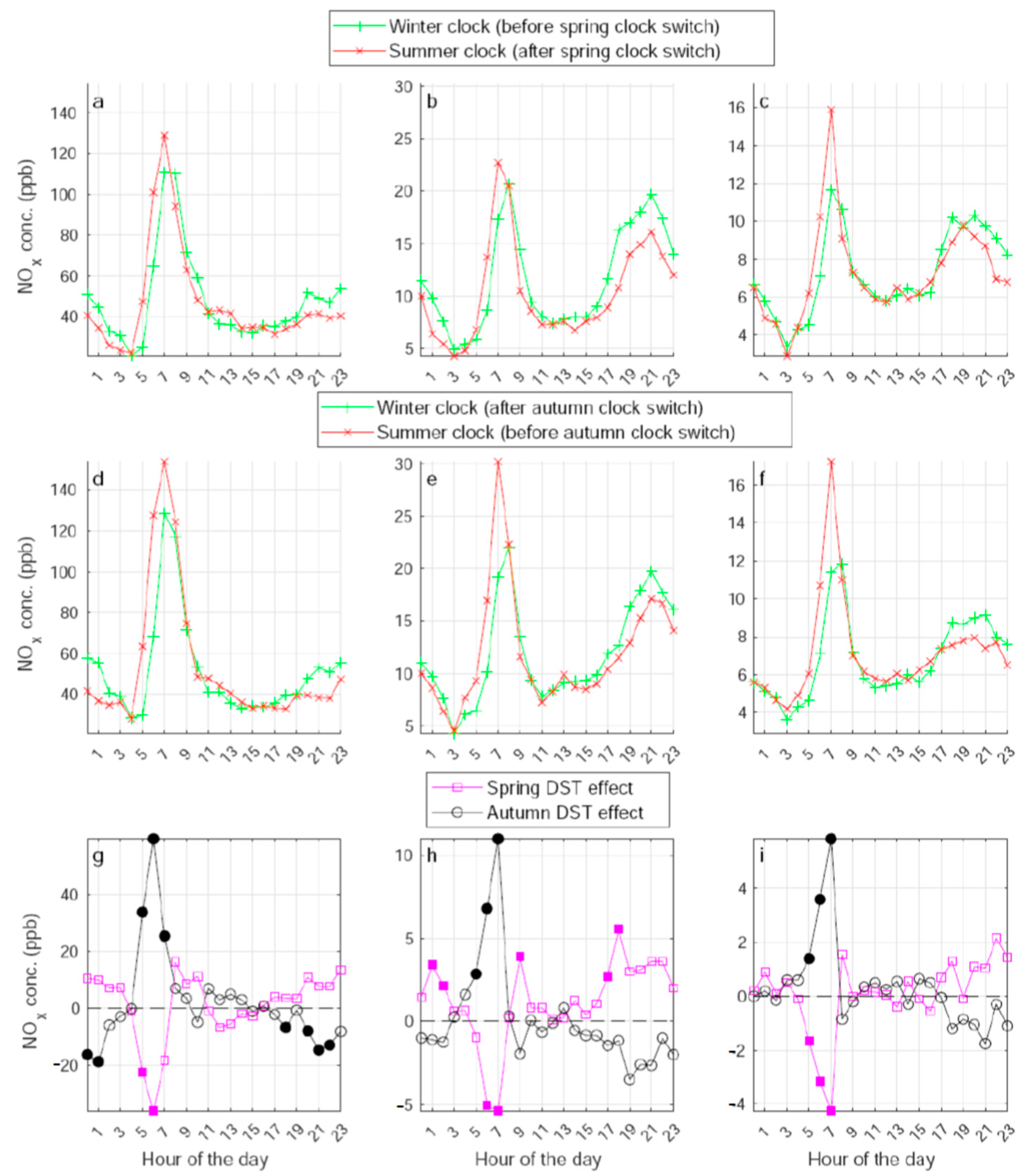
Figure 3 depicts the DST effect on NOx concentrations in three AQM stations, showing daily cycles of average NOx concentrations in five working days before and after the spring and autumn DST clock changes. The Remez AQM station (left column in Figure 3) is a transportation AQM station at the heart of Israel’s largest conurbation—Gush Dan, situated five km from the shoreline at elevation of 20 m a.s.l. The AQM station surrounding area experienced morning to late afternoon car and truck volumes of about 3500 and 250 vehicles per hour, respectively. The Bet Shemesh AQN station (middle column) is located in a mid-size city (population 140,000 in 2018), 35 km from the shoreline and at elevation of 305 m a.s.l. The AQM station experienced a morning (around 08:00 a.m.) peak of car and truck volumes of about 900 and 50 vehicles per hour, respectively. The Karmiel AQM station is the northern AQM station examined in this study, situated in a small city in the western Galilee (population 45,000 in 2018) at elevation of 350 m a.s.l. It experienced a 08:00 a.m. peak volumes of 500 and 50 cars and trucks per hour, respectively. Nonetheless, despite the very different characteristics of the three AQM stations and the very large differences in NOx concentrations which they observed, the shapes of the daily NOx concentration cycles are very similar. Specifically, the NOx concentrations at the three AQM stations show a steep increase in the morning, followed by a similar sharp decrease towards noon. A second but much smaller NOx concentration peak is noted at the three AQM stations in the evening, characterized by a more gradual concentrations increase and decline. As could be expected, the summertime concentration cycles are shifted an hour earlier compared to the winter ones. Interestingly, summertime concentrations in the morning were much higher than the comparable wintertime concentrations. In contrast, in the evening they were lower, although the difference was smaller. It is noteworthy that the shapes of the DST effects in the three AQM stations (Figure 3g–i) were very similar. Table 1 demonstrates that the shapes of the DST effects were similar at other AQM stations as well, with the median correlation between the NOx DST effect curves across all pairs of AQM stations with sufficient data being 0.63 and 0.71 for the spring and autumn DST clock changes, respectively.
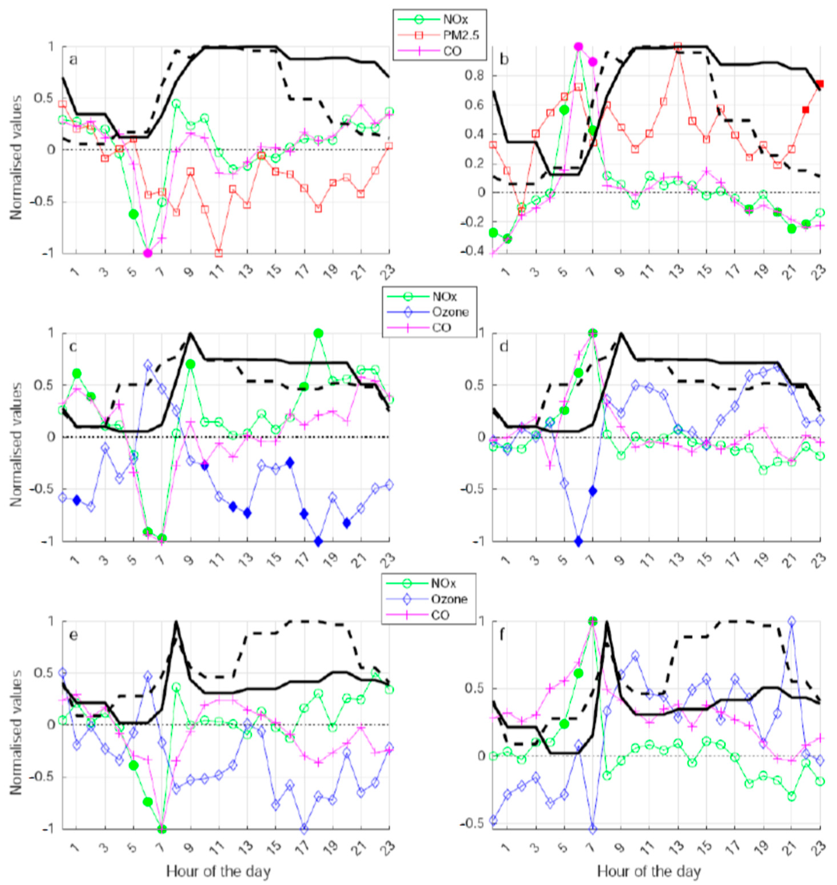
Figure 4 presents the DST effect for NOx, CO, O3 and PM2.5 in AQM stations Remez, Bet Shemesh and Karmiel (the same stations whose data were shown in Figure 3). Each of these AQM stations has observed only three of the studied pollutants for long enough time periods to be included in this analysis. Also shown in Figure 4 are the daily cycles of car and truck volumes near the AQM stations. To present all the daily cycles in each plot using a common y-axis, the variables were normalized by dividing the original values of each variable by its maximal value. The curves of the normalized NOx and CO DST effects are quite similar, with their morning extrema occurring at the same time. The curves that depict the DST effect of O3 (middle and lower rows in Figure 4) show an opposite pattern to the general patterns of the NOx and CO DST effects. The PM2.5 DST effect in AQM station Remez (upper row in Figure 4) does not show much association with those of the two other pollutants. Table 2 shows that the correlations between the DST effect of NOx and that of each of the other pollutants (Figure 4) are consistent across the whole study area. The correlations between the NOx and CO DST effects in AQM stations that observe both pollutants were moderate–high and positive. The correlations between the NOx and O3 DST effects were moderate–high and negative. The correlations between the NOx and PM2.5 DST effects were much lower. It is well-known that in areas where O3 formation takes place under a VOC-limited regime, i.e., where ambient levels of VOC rather than those of NOx govern the ambient ozone levels, similar negative correlations are observed [20]. In general, ozone formation in the study area was found to take place under a VOC-limited regime [21,22,23].
Most notable in Figure 4 is that the timing of the peaks and troughs in the DST effect curves, which occurred almost simultaneously for NOx, CO and O3, did not coincide with the daily cycles of the car and truck volumes. For example, in AQM station Remez the peaks (autumn) and troughs (spring) of the DST effects of NOx and CO occurred at 06:00 a.m., when the car and truck volumes were still at, or very close to, their minimum levels. In general, local emissions of NOx and CO in the study area emanate from diesel trucks and petrol cars, respectively. Yet, it is clear from Figure 4 that the observed concentrations of NOx and CO have been affected also by other factors that occurred at similar times all over the study area (i.e., not locally). In particular, the variability in the normalized NOx and CO concentrations in the morning hours around the spring and autumn DST clock changes could not have been resulted solely by abrupt time shifts in traffic volumes (i.e., due to the effect of DST change on anthropogenic emissions). Meteorology is an additional factor that could result in the observed DST effects.
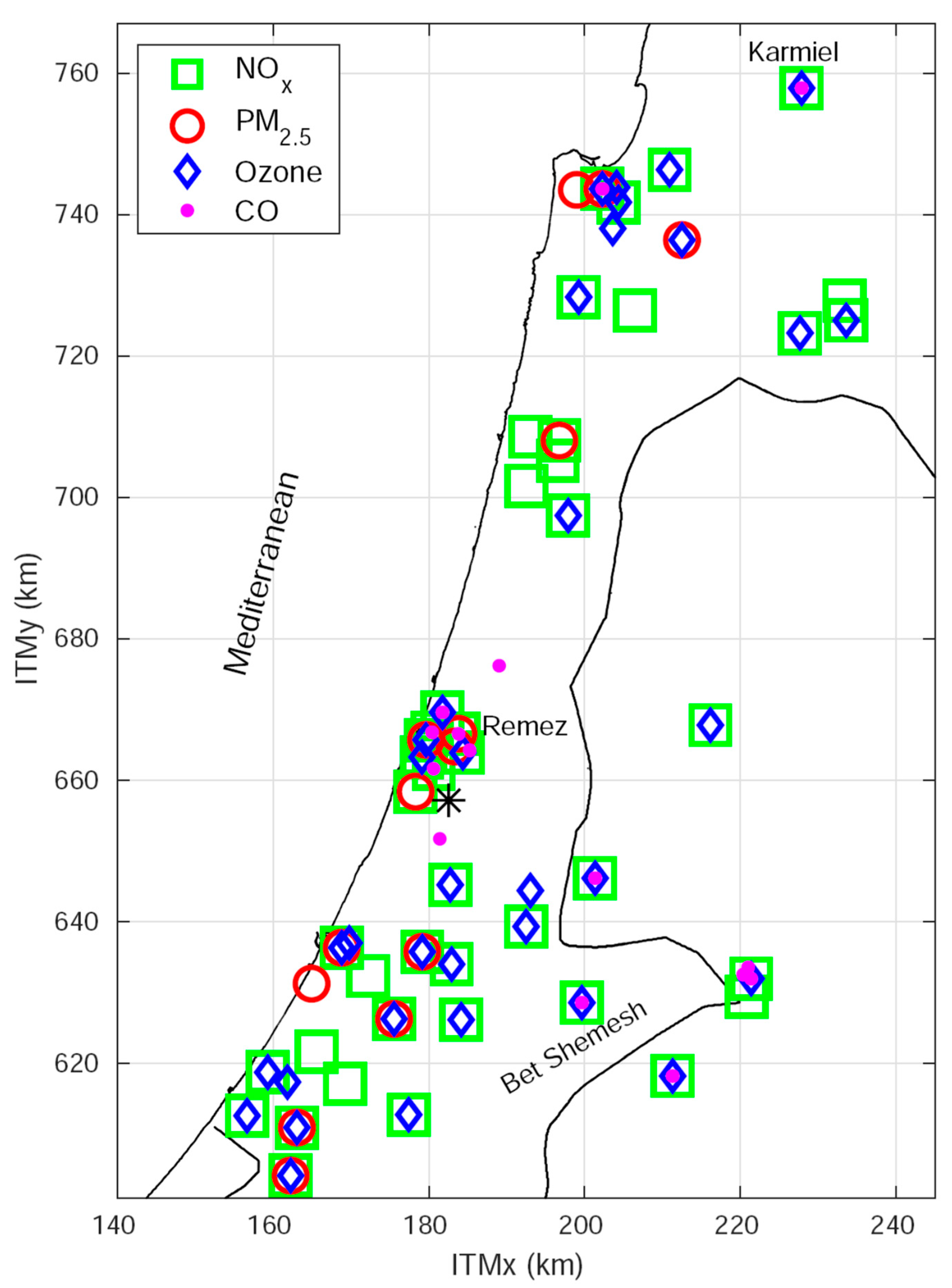
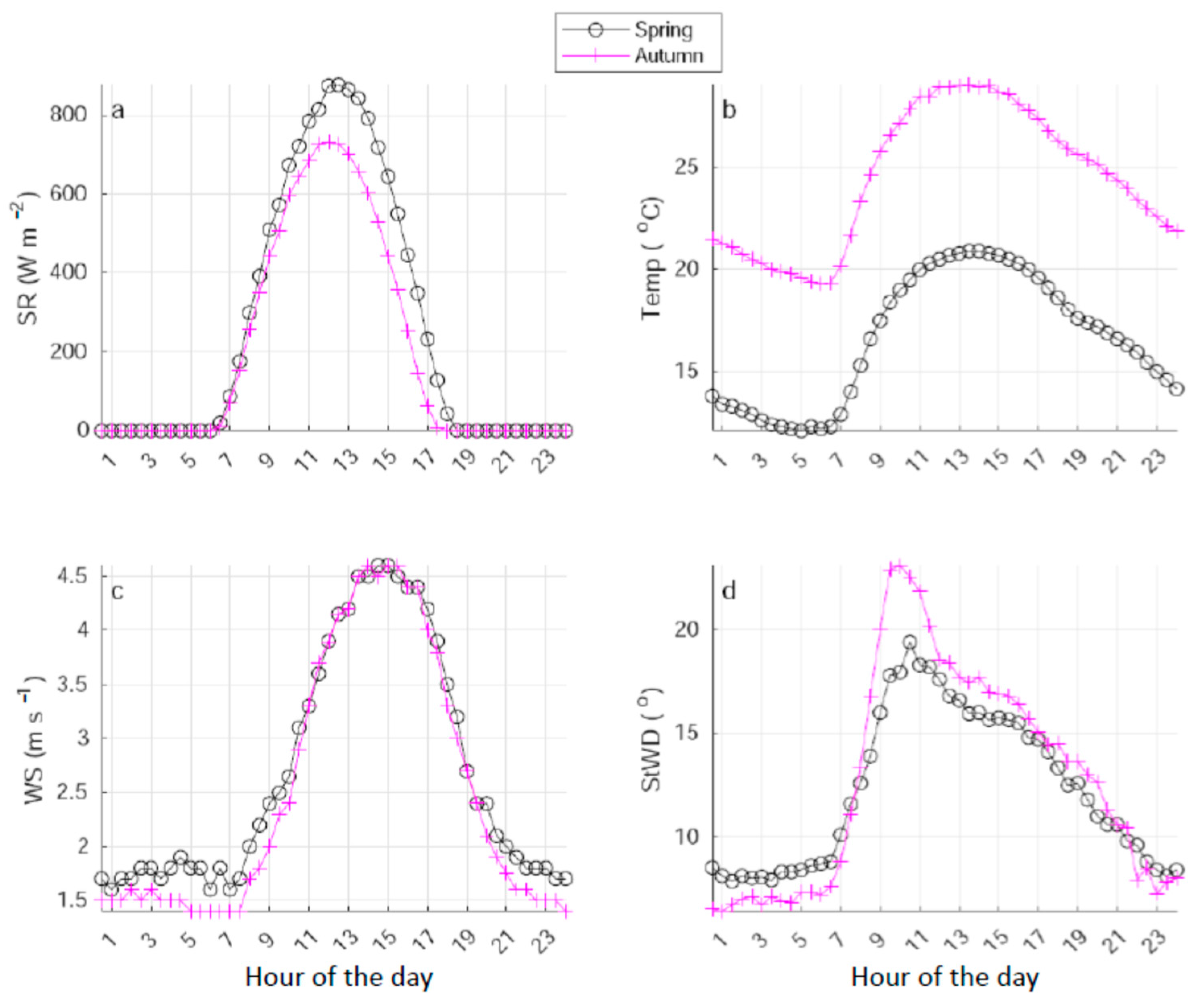
Figure 5 shows the daily cycles of the temperature, solar radiation, wind speed and standard deviation of the wind direction at the Bet Dagan meteorological station, which is located at the center of the study area (Figure 1). Sunrise at both DST clock change days is around 07:00 a.m. The ambient temperature is at its minimum just before sunrise and starts to increase rapidly immediately after. The temperature in the morning is highly correlated with the temperature lapse rate, which has been shown to have a strong negative association with primary pollutant concentrations in the study area [7]. The wind speed and the standard deviation of the wind direction are two common proxies of turbulence, which was also shown to be negatively associated with pollutant concentrations [8], and which also starts to rapidly intensify after sunrise. Thus, the strong morning DST effect coincides with rapid changes in three meteorological factors that are commonly associated with pollutant dispersion: lapse rate/buoyancy, turbulence, and wind shear. The more subtle evening DST effect is probably due to the more gradual afternoon decrease in the intensities of these meteorological factors (Figure 5). Both the morning and evening DST effects are opposite in sign in the spring and in the autumn due to the opposite DST clock changes. The NOx and CO DST effects (Figure 4) seem to be impacted by meteorology beyond the effect of the morning and evening peak traffic emissions shift one hour ahead or backward.
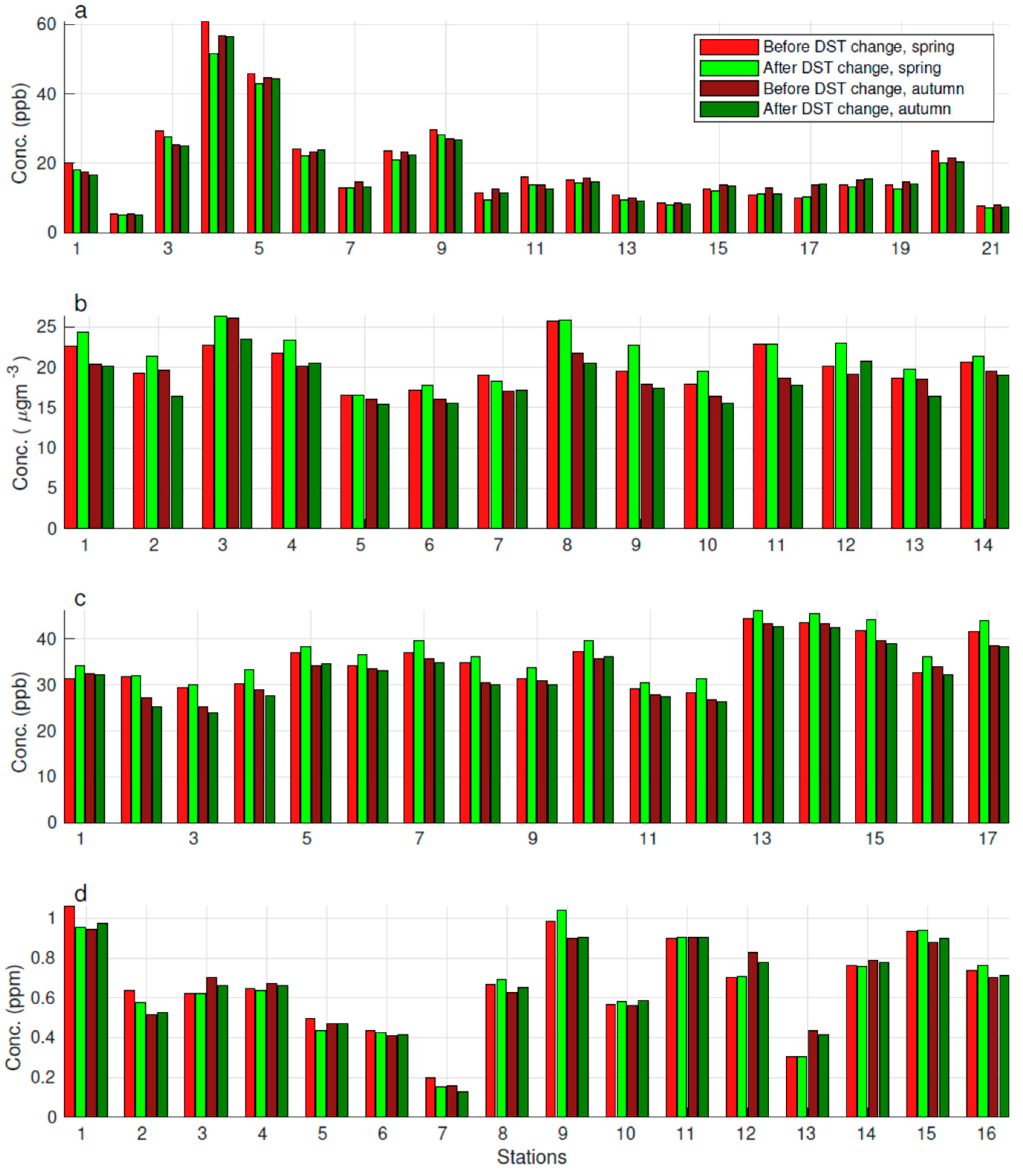
While Figure 3 depicts a strong but short morning DST effect, and a longer, opposite in sign, and less intense evening DST effect, Figure 6 shows that the morning and evening DST effects tend to cancel out each other such that at most AQM stations and for most of the pollutants examined the mean daily pollutant concentrations experienced before either of the DST changes were very similar to those experienced after the DST changes. The only consistent exception is the spring daily mean O3 concentrations, which are always higher after the DST clock change than before it. This probably results from the rapid spring-time temperature change, which affects the rates of photochemical and oxidation reactions that participate in O3 formation and destruction. However, even in this case the differences between the concentrations before and after the DST change are small.

4. Discussion

Variation in traffic emissions is the main anthropogenic contributor to the temporal variability in NOx and CO concentrations in Israel. Due to traffic-related VOC emissions in parallel to the NOx emissions, the variability in traffic volumes is also responsible for spatial variation in daytime O3 concentrations. Namely, the early morning rise in traffic volumes initiates a corresponding rise in NOx and CO concentrations, and a decrease in O3 concentration due to titration of its background values (i.e., ozone is consumed during the oxidation of NO to NO2). Our results demonstrate that while DST clock changes do not affect the intensity of emissions nor of dispersion processes, they do affect observed traffic related air pollution (TRAP) concentrations beyond what could have been expected. This is due to the shift in the emissions one hour forward or backward, with respect to UTC. Unlike the timing of anthropogenic emissions, the timing of dispersion processes is blind to DST changes. It is well-known that primary (secondary) pollutants attain their ambient concentrations as a result of delicate interactions between their emissions (formation) and co-occurring dispersion conditions and removal processes. In particular, TRAP results not only by (DST-modified) rush hour vehicle emissions but also by (DST-neutral) dispersion-reaction processes, which are governed to a large degree by the prevailing meteorological conditions.
Yuval et al. [7] showed that pre-sunrise pollutant levels are mainly determined by the intensity of the nocturnal atmospheric stability. The current work demonstrates that while the DST-affected traffic emissions are prerequisite for TRAP, the daily dynamics of TRAP patterns, in particular the timing of the peak concentrations, is synergistically related to various meteorological conditions, in particular the sunrise time. This is most noticeable around the autumn DST clock change (Figure 4 right column), when the NOx DST effect in the morning rises considerably before sunrise (Figure 5a, i.e., higher concentrations before the wintertime clock change than after it) while there is no change (and even decrease) in diesel vehicle volumes, which are the main source of traffic NOx emissions. Similarly, around the spring DST clock change (Figure 4 left column) the CO DST effect in the morning falls considerably before sunrise even at AQM stations where petrol vehicle volumes, the main source of traffic CO emissions, were soaring. Moreover, the timing of the morning peak (trough) of the O3 DST effect in the spring (autumn) DST daily cycle (Figure 4), which is negatively correlated with those of the primary pollutants (since ozone is a secondary pollutant), also attest on the major impact of meteorological variables, especially the sunrise time, on ambient pollutant concentrations.
The DST effect was noted in all the urban AQM stations where peak vehicle volumes exceeded 200 cars or 20 trucks per hour and was significant enough to be noted also in the concentrations of O3. However, in some of the rural AQM stations, mostly away from the coast, the effect was negligible or not noted at all. We believe that at these sites, the DST effect is masked by pollutant concentrations that are transported by the daytime westerly winds from upwind urban centers, which are situated in Israel mostly along the shoreline. Moreover, we did not notice a clear PM2.5 DST effect, which suggests relatively little impact of traffic emissions on PM2.5 concentrations in Israel, in agreement with [8]. A large fraction of the observed PM2.5 in the eastern Mediterranean is due to transboundary transport from Europe, North Africa, and the Arabian Peninsula [24], and naturally these sources are not impacted by DST clock changes in Israel.
The daily average concentrations of the examined pollutants have not changed significantly following the DST clock changes. The general population is thus probably unaffected by exposure-related DST changes. Yet, people that are exposed to outdoor pollutants mostly in the morning or in the evening might experience a notable effect. For example, pupils and staff, especially of schools that are located near busy roads, may be exposed to much higher morning NOx and CO concentrations during summer DST clock (Figure 3), while commuting to school, with the effect not cancelled out if they spend most of their evening hours indoors or in residential neighborhoods with low traffic volumes. On the other hand, the health benefits of longer leisure time, enabled by the spring DST clock change, especially when sport activities are exercised, are probably enhanced due to the lower summer DST clock evening pollutant concentrations. Furthermore, the DST effects which we noted in spring and autumn probably become less significant as time proceed towards the solstices, especially at high latitudes. In the summer, the reason for this is the early sunrise that results in breaking of the stable nocturnal atmospheric boundary layer, and a higher daytime turbulence early in the morning. Both processes result in destruction of pollutant concentrations buildup. An opposite effect occurs in winter, since meteorological processes that enable effective pollutant dispersion do not commence early enough to destruct the accumulation of pollutant near the surface, which results in noticeable concentration peaks even when inchoate morning traffic volume conditions are experienced.

5. Conclusions

This study exploits the natural experiments enabled by the DST clock changes twice a year, to better understand the interplay between pollutant emissions and meteorological processes that govern pollutant dispersion and removal. The DST clock changes introduce a perturbation (abrupt time shift) into the pollutant emission-dispersion processes, with the former DST-affected and the latter DST-blind. We found a strong correlation between the DST effect and traffic-related primary pollutant (NOx and CO) concentrations, which could not be explained by the shift in vehicle volumes in response to the DST impact on daily human activities (vehicle emissions are the main local source of these pollutants). Moreover, while a DST effect was found also for ambient O3 concentrations (a secondary pollutant), a PM2.5 DST effect has not been found. This suggests that traffic emissions have a relatively little impact on PM2.5 concentrations in Israel, in agreement with [8]. In the eastern Mediterranean transboundary transport is a major source of PM2.5. While meteorology is basically DST-blind, anthropogenic emissions that do not emanate 24/7 are by-nature DST-affected. Together, these factors act in synergy and their effects show considerable spatiotemporal variability.
We found no clear impact of DST clock changes on the overall daily mean concentrations of the four pollutants examined (NOx, CO, O3, PM2.5), with possible disadvantages (benefits) for specific population groups that spend distinct time-intervals outdoors or during commute. In many countries, the practice of DST is under debate, with the tendency to cancel its obligatory adoption [25]. Our findings suggest that canceling the DST clock change practice will probably cause negligible effects on the daily average pollutant concentrations, as well as on the averages of pollutant concentrations over longer periods. Yet, (repeating) short-term exposure may result in small and varied effects in certain population subgroups, depending on their specific time-location-activity trajectories. The tools and viewpoint presented in this work, once applied on local data, may serve as an additional input to decision makers while considering whether to continue the DST practice, and if the choice is to adopt a fixed clock which one to choose: winter or summer. For Israel, our study area, we found that DST changes are not expected to affect the overall daily exposure to TRAP and, as such, may not contribute, by itself, to the decision where to continue the practice of DST clock changes. However, our neutral results may support a decision to halt DST clock changes due to other reasons and, instead, adopt a fixed clock (which would probably be the DST/summertime).

Author Contributions

Conceptualization, Y., Y.L. and D.M.B.; methodology, Y.; software, Y.; validation, Y., Y.L. and D.M.B.; formal analysis, Y.; investigation, Y.; resources, D.M.B.; data curation, Y.; writing—original draft preparation, Y.; writing—review and editing, Y., Y.L. and D.M.B.; visualization, Y.; supervision, D.M.B.; project administration, D.M.B. All authors have read and agreed to the published version of the manuscript.

Funding

This research received no external funding.

Institutional Review Board Statement

Not applicable.

Informed Consent Statement

Not applicable.

Data Availability Statement

The air quality data presented in this study are available from the Israeli Air Quality Monitoring Center website, http://www.svivaaqm.net/Default.rtl.aspx, accessed on 1 March 2022. The meteorological data were obtained from the Israeli Meteorological Service website, https://ims.data.gov.il/ims/7, accessed on 1 March 2022. The traffic volumes were obtained from Decell Technologies and can be provided upon request.

Acknowledgments

This research was performed at the Technion Center of Excellence in Exposure Science and Environmental Health (TCEEH).

Conflicts of Interest

The authors declare no conflict of interest.

References

  1. Havranek, T.; Herman, D.; Irsova, Z. Does Daylight Saving Save Electricity? A Meta-Analysis. Energy J. 2018, 39, 35–61. [Google Scholar] [CrossRef]
  2. Toro, W.; Tigre, R.; Sampaio, B. Daylight Saving Time and incidence of myocardial infarction: Evidence from a regression discontinuity design. Econ. Lett. 2015, 136, 1–4. [Google Scholar] [CrossRef]
  3. Poteser, M.; Moshammer, H. Daylight saving time transitions: Impact on total mortality. Int. J. Environ. Res. Public Health 2020, 17, 1611. [Google Scholar] [CrossRef]
  4. Prats–Uribe, A.; Tobías, A.; Prieto–Alhambra, D. Excess risk of fatal road trac accidents on the day of daylight saving time change. Epidemiology 2018, 29, e44–e45. [Google Scholar] [CrossRef]
  5. Goodman, A.; Page, A.S.; Cooper, A.R. Daylight saving time as a potential public health intervention: An observational study of evening daylight and objectively–measured physical activity among 23,000 children from 9 countries. Int. J. Behav. Nutr. Phys. Act. 2014, 11, 84. [Google Scholar] [CrossRef] [PubMed]
  6. Seo, J.; Park, D.R.; Kim, J.Y.; Youn, D.; Lim, Y.B.; Kim, Y. Effects of meteorology and emissions on urban air quality: A quantitative statistical approach to long–term records (1999–2016) in Seoul, South Korea. Atmos. Chem. Phys. 2018, 18, 16121–16137. [Google Scholar] [CrossRef]
  7. Yuval; Levi, Y.; Dayan, U.; Levy, I.; Broday, D.M. On the association between characteristics of the atmospheric boundary layer and air pollution concentrations. Atmos. Res. 2020, 231, 104675. [Google Scholar] [CrossRef]
  8. Yuval; Trischer, T.; Raz, R.; Levi, Y.; Levy, I.; Broday, D.M. Emissions vs. turbulence and atmospheric stability: A study of their relative importance in determining air pollutant concentrations. Sci. Total Environ. 2020, 733, 139300. [Google Scholar] [CrossRef]
  9. Muñoz, R. Relative roles of emissions and meteorology in the diurnal pattern of urban PM10: Analysis of the daylight saving time effect. J. Air Waste Manag. Assoc. 2012, 62, 642–650. [Google Scholar] [CrossRef]
  10. Sullivan, J.M.; Flannagan, M.J. The role of ambient light level in fatal crashes: Inferences from daylight saving time transitions. Accid. Anal. Prev. 2002, 34, 487–498. [Google Scholar] [CrossRef]
  11. Hadlow, N.C.; Brown, S.; Wardrop, R.; Henley, D. The effects of season, daylight saving and time of sunrise on serum cortisol in a large population. J. Biol. Med. Rhythm Res. 2014, 31, 243–251. [Google Scholar] [CrossRef] [PubMed]
  12. Cohen, J. A statistical analysis of the effect of time shifting automobile emissions on ambient ozone concentrations. In Proceedings of the Transactions of the 5th International Specialty Conference on Ozone, Los Angeles, CA, USA, 19–22 March 1990; pp. 850–861. [Google Scholar]
  13. Hecq, W.; Borisov, Y.; Totte, M. Daylight saving time effect on fuel consumption and atmospheric pollution. Sci. Total Environ. 1993, 133, 249–274. [Google Scholar] [CrossRef]
  14. Chen, S.; Yuavl; Broday, D.M. Re–framing the Gaussian dispersion model as a nonlinear regression scheme for retrospective air quality assessment at a high spatial and temporal resolution. Environ. Model. Softw. 2020, 125, 104620. [Google Scholar] [CrossRef]
  15. Dayan, U.; Levy, I. Relationship between synoptic-scale atmospheric circulation and ozone concentration over Israel. J. Geophys. Res. Atmos. 2002, 107, ACL-31. [Google Scholar] [CrossRef]
  16. Levy, I.; Mahrer, Y.; Dayan, U. Coastal and synoptic recirculation affecting air pollutants dispersion: A numerical study. Atmos. Environ. 2009, 43, 1991–1999. [Google Scholar] [CrossRef]
  17. Bekhor, S.; Lotan, T.; Gitelman, V.; Morik, S. Free–flow travel speed analysis and monitoring at the national level using global positioning system measurements. J. Transp. Eng. 2013, 139, 1235–1243. [Google Scholar] [CrossRef]
  18. Chen, S.; Yuavl; Broday, D.M. Aggregated GPS tracking of vehicles and its use as a proxy of traffic-related air pollution emissions. Atmos. Environ. 2016, 142, 351–359. [Google Scholar] [CrossRef]
  19. Gibbons, J.D.; Chakraborti, S. Nonparametric Statistical Inference, 5th ed.; CRC Press, Taylor & Francis Group: Boca Raton, FL, USA, 2011. [Google Scholar]
  20. Seinfeld, J.H.; Pandis, S.N. Atmospheric Chemistry and Physics: From Air Pollution to Climate Change, 3rd ed.; John Wiley & Sons: New York, NY, USA, 2016. [Google Scholar]
  21. Yuval; Broday, D.M. High resolution spatial patterns of long-term mean air pollutants concentrations in Haifa Bay area. Atmos. Environ. 2006, 40, 3653–3664. [Google Scholar] [CrossRef]
  22. Yuval; Flicstein, B.; Broday, D.M. The impact of reduced traffic volumes on urban air pollution. Atmos. Environ. 2008, 42, 428–440. [Google Scholar] [CrossRef]
  23. Yuval; Broday, D.M. Studying the time scale dependence of environmental variables predictability using fractal analysis. Environ. Sci. Technol. 2010, 44, 4629–4634. [Google Scholar]
  24. Kalderon–Asael, B.; Erel, Y.; Sandler, A.; Dayan, U. Mineralogical and chemical characterization of suspended atmospheric particles over the east Mediterranean based on synoptic scale circulation patterns. Atmos. Environ. 2009, 43, 3963–3970. [Google Scholar] [CrossRef]
  25. Commission of the European Communities. Proposal for a Directive of the European Parliament and of the Council Discontinuing Seasonal Changes of Time and Repealing Directive 2000/84/EC. COM/2018/639 2018, Final; European Commission: Brussels, Belgium, 2018. [Google Scholar]
Figure 1. The study area and the spatial distribution of the air quality monitoring (AQM) stations from which the observations of NOx, PM2.5, O3 and CO were gathered. The black asterisk denotes the location of the Bet Dagan meteorological station. The coordinates are in the Israeli Transverse Mercator (ITM) projection.
Atmosphere 13 01458 g001
Figure 2. The 2000–2020 dates of DST clock changes (red dots), with five days periods before and after them marked by thin black lines (see Section 2.3) and the Jewish holiday periods marked by thick cyan lines. (a) Spring DST; (b) autumn DST. The vertical dotted lines denote the spring and autumn equinox days.
Atmosphere 13 01458 g002
Figure 3. Daily cycles of NOx, averaged over five working days before and after the DST clock changes, at AQM stations Remez (left column), Bet Shemesh (middle column), and Karmiel (right column) (see Figure 1). Upper row (ac)—daily NOx concentration cycles in the spring; middle row (df)—daily NOx concentration cycles in the autumn; lower row (gi)—daily cycles of the DST effect (the difference between the median NOx concentrations before and after the DST clock change at corresponding hours of the day). Filled symbols denote differences that are statistically significant at the p = 0.01 level.
Atmosphere 13 01458 g003
Figure 4. Normalized daily cycles of the DST effect of all the pollutants observed at AQM stations Remez (upper row, subfigures (a,b)), Bet Shemesh (middle row, subfigures (c,d)) and Karmiel (lower row, subfigures (e,f)). Only cycles based on at least 15 years (10 in the case of CO) were considered. Filled markers denote time points where the DST effect was statistically significant at the p = 0.01 level. Normalized daily cycles of car (continuous black line) and truck (dashed black line) volumes near the AQM stations are also shown. Left column: spring DST clock change, and right column: autumn DST clock change.
Atmosphere 13 01458 g004
Figure 5. Daily cycles of meteorological variables, averaged over five working days before and after the spring and autumn DST clock changes in 2000–2020. The meteorological variables, (a)—solar radiation (SR), (b)—temperature (Temp), (c)—wind speed (WS) and (d)—standard deviation of the wind direction (SWD), were observed at the Bet Dagan meteorological station, which is located at the center of the study area (Figure 1).
Atmosphere 13 01458 g005
Figure 6. Mean concentrations during five working days before and after the DST changes. (a) NOx, (b) PM2.5, (c) O3 and (d) CO. For visual purposes, the x-axes labels of the NOx and O3 plots contain only odd numbers.
Atmosphere 13 01458 g006
Table 1. Medians of the correlations between the DST effects observed at different AQM station pairs. The distribution of the correlations for each pollutant contains the correlations between all the combinations of AQM station pairs (N) that experienced peak traffic volumes of at least 200 cars or 20 trucks per hour.
PollutantNo. of AQM StationsNMedian Corr. SpringMedian Corr. Autumn
NOx283780.630.71
CO14910.570.74
Ozone232530.430.47
PM2.510450.200.05
Table 2. Median correlation between the DST effect of NOx and of the other pollutants. NOx is observed at most of the AQM stations in the study area. Its spring and autumn DST effects in each AQM station were correlated with the corresponding DST effects of the other pollutants that were observed at the same AQM station. At least 15 years (10 in the case of CO) of data were required for the AQM station data to be included in the analysis.
PM2.5O3CO
No. of pollutant pairs102911
Spring DST effect0.10−0.720.75
Autumn DST effect0.27−0.760.83
Publisher’s Note: MDPI stays neutral with regard to jurisdictional claims in published maps and institutional affiliations.

