
Modeling PM2.5 and PM10 Using a Robust Simplified Linear Regression Machine Learning Algorithm


Abstract
:1. Introduction
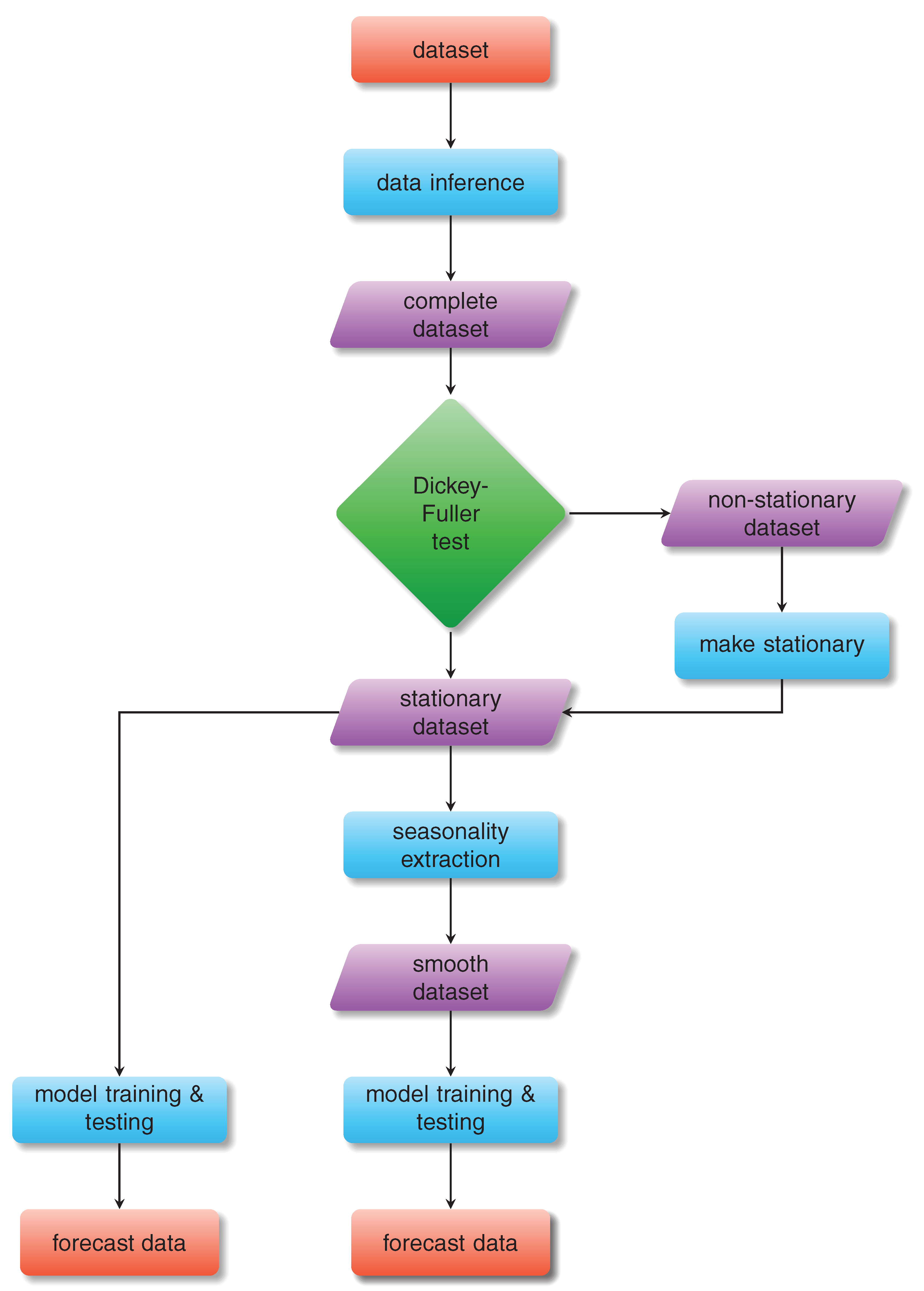
2. Data and Methods
| Algorithm 1: Multiple-input multiple-output linear regression algorithm. |
 |
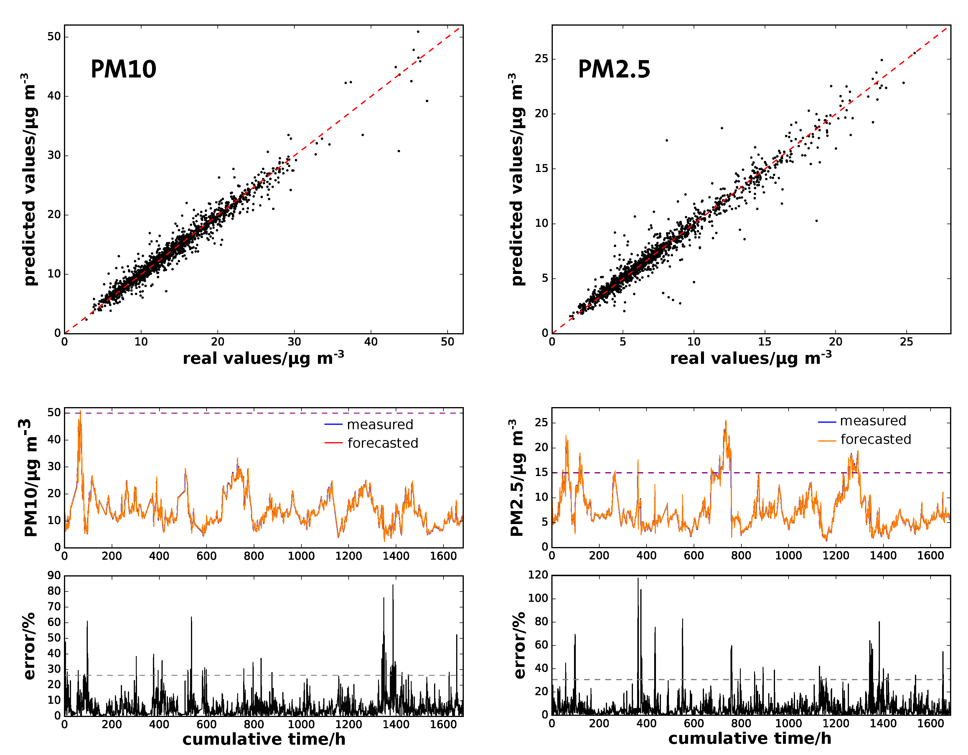
3. Results and Discussion
3.1. Original Data
3.2. Seasonal Decomposed Data
3.3. Statistical Analysis
4. Conclusions
Author Contributions
Funding
Institutional Review Board Statement
Informed Consent Statement
Data Availability Statement
Conflicts of Interest
References
- World Health Statistics 2022: Monitoring Health for the SDGs, Sustainable Development Goals; World Health Organization: Geneve, Switzerland, 2022.
- Wang, L.; Zhong, B.; Vardoulakis, S.; Zhang, F.; Pilot, E.; Li, Y.; Yang, L.; Wang, W.; Krafft, T. Air Quality Strategies on Public Health and Health Equity in Europe—A Systematic Review. Int. J. Environ. Res. Public Health 2016, 13, 1196. [Google Scholar] [CrossRef] [PubMed] [Green Version]
- Chu, Y.; Liu, Y.; Li, X.; Liu, Z.; Lu, H.; Lu, Y.; Mao, Z.; Chen, X.; Li, N.; Ren, M.; et al. A Review on Predicting Ground PM2.5 Concentration Using Satellite Aerosol Optical Depth. Atmosphere 2016, 7, 129. [Google Scholar] [CrossRef] [Green Version]
- Leung, D.Y. Outdoor-indoor air pollution in urban environment: Challenges and opportunity. Front. Environ. Sci. 2015, 2, 69. [Google Scholar] [CrossRef]
- Katsouyanni, K. Ambient air pollution and health. Br. Med. Bull. 2003, 68, 143–156. [Google Scholar] [CrossRef] [Green Version]
- Macintyre, H.L.; Heaviside, C.; Neal, L.S.; Agnew, P.; Thornes, J.; Vardoulakis, S. Mortality and emergency hospitalizations associated with atmospheric particulate matter episodes across the UK in spring 2014. Environ. Int. 2016, 97, 108–116. [Google Scholar] [CrossRef]
- Xie, R.; Sabel, C.E.; Lu, X.; Zhu, W.; Kan, H.; Nielsen, C.P.; Wang, H. Long-term trend and spatial pattern of PM 2.5 induced premature mortality in China. Environ. Int. 2016, 97, 180–186. [Google Scholar] [CrossRef]
- De Mattos Neto, P.S.; Cavalcanti, G.D.; Madeiro, F.; Ferreira, T.A. An Approach to Improve the Performance of PM Forecasters. PLoS ONE 2015, 10, e0138507. [Google Scholar] [CrossRef] [Green Version]
- Gautam, S.; Yadav, A.; Tsai, C.J.; Kumar, P. A review on recent progress in observations, sources, classification and regulations of PM2.5 in Asian environments. Environ. Sci. Pollut. Res. 2016, 23, 21165–21175. [Google Scholar] [CrossRef]
- Fajersztajn, L.; Veras, M.; Barrozo, L.V.; Saldiva, P. Air pollution: A potentially modifiable risk factor for lung cancer. Nat. Rev. Cancer 2013, 13, 674–678. [Google Scholar] [CrossRef]
- Feng, J.; Yang, W. Effects of Particulate Air Pollution on Cardiovascular Health: A Population Health Risk Assessment. PLoS ONE 2012, 7, e33385. [Google Scholar] [CrossRef] [Green Version]
- Kim, H.; Kim, W.H.; Kim, Y.Y.; Park, H.Y. Air Pollution and Central Nervous System Disease: A Review of the Impact of Fine Particulate Matter on Neurological Disorders. Front. Public Health 2020, 8, 921. [Google Scholar] [CrossRef]
- Sîrbu, C.A.; Stefan, I.; Dumitru, R.; Mitrica, M.; Manole, A.M.; Vasile, T.M.; Stefani, C.; Ranetti, A.E. Air Pollution and Its Devastating Effects on the Central Nervous System. Healthcare 2022, 10, 1170. [Google Scholar] [CrossRef]
- Breitner, S.; Schneider, A.; Devlin, R.B.; Ward-Caviness, C.K.; Diaz-Sanchez, D.; Neas, L.M.; Cascio, W.E.; Peters, A.; Hauser, E.R.; Shah, S.H.; et al. Associations among plasma metabolite levels and short-term exposure to PM2.5 and ozone in a cardiac catheterization cohort. Environ. Int. 2016, 97, 76–84. [Google Scholar] [CrossRef] [Green Version]
- Gozzi, F.; Della Ventura, G.; Marcelli, A. Mobile monitoring of particulate matter: State of art and perspectives. Atmos. Poll. Res. 2016, 7, 228–234. [Google Scholar] [CrossRef]
- Marcazzan, G.M.; Vaccaro, S.; Valli, G.; Vecchi, R. Characterisation of PM10 and PM2.5 particulate matter in the ambient air of Milan (Italy). Atmos. Environ. 2001, 35, 4639–4650. [Google Scholar] [CrossRef]
- Wallace, L.; Bi, J.; Ott, W.R.; Sarnat, J.; Liu, Y. Calibration of low-cost PurpleAir outdoor monitors using an improved method of calculating PM2.5. Atmos. Environ. 2021, 256, 118432. [Google Scholar] [CrossRef]
- Spurny, K.R. Aerosol Filstration and Sampling. In Advances in Aerosol Filtration; Spurny, K.R., Ed.; CRC Press: Boca Raton, FL, USA, 1998; p. 415. [Google Scholar]
- Harrison, R.M.; Deacon, A.R.; Jones, M.R.; Appleby, R.S. Sources and processes affecting concentrations of PM10 and PM2.5 particulate matter in Birmingham (U.K.). Atmos. Environ. 1997, 31, 4103–4117. [Google Scholar] [CrossRef]
- Querol, X.; Alastuey, A.; Ruiz, C.R.; Artiñano, B.; Hansson, H.C.; Harrison, R.M.; Buringh, E.; Ten Brink, H.M.; Lutz, M.; Bruckmann, P.; et al. Speciation and origin of PM10 and PM2.5 in selected European cities. Atmos. Environ. 2004, 38, 6547–6555. [Google Scholar] [CrossRef]
- Wilks, D.S. Statistics. Stat. Methods Atmos. Sci. 2011, 100, 100. [Google Scholar]
- Lynch, P. The origins of computer weather prediction and climate modeling. J. Comp. Phys. 2008, 227, 3431–3444. [Google Scholar] [CrossRef] [Green Version]
- Nazif, A.; Mohammed, N.I.; Malakahmad, A.; Abualqumboz, M.S. Application of Step Wise Regression Analysis in Predicting Future Particulate Matter Concentration Episode. Water Air Soil Pollut. 2016, 227, 117. [Google Scholar] [CrossRef]
- Ben Taieb, S.; Bontempi, G.; Atiya, A.F.; Sorjamaa, A. A review and comparison of strategies for multi-step ahead time series forecasting based on the NN5 forecasting competition. Expert Syst. Appl. 2012, 39, 7067–7083. [Google Scholar] [CrossRef] [Green Version]
- Pérez, P.; Trier, A.; Reyes, J. Prediction of PM2.5 concentrations several hours in advance using neural networks in Santiago, Chile. Atmos. Environ. 2000, 34, 1189–1196. [Google Scholar] [CrossRef]
- Sfetsos, A.; Vlachogiannis, D. Time Series Forecasting of Hourly PM10 Using Localized Linear Models. J. Soft. Eng. App. 2010, 3, 374–383. [Google Scholar] [CrossRef] [Green Version]
- Cabaneros, S.M.; Calautit, J.K.; Hughes, B.R. A review of artificial neural network models for ambient air pollution prediction. Environ. Mod. Soft. 2019, 119, 285–304. [Google Scholar] [CrossRef]
- Kalajdjieski, J.; Zdravevski, E.; Corizzo, R.; Lameski, P.; Kalajdziski, S.; Pires, I.M.; Garcia, N.M.; Trajkovik, V. Air Pollution Prediction with Multi-Modal Data and Deep Neural Networks. Remote Sens. 2020, 12, 4142. [Google Scholar] [CrossRef]
- Fan, J.; Li, Q.; Hou, J.; Feng, X.; Karimian, H.; Lin, S. A spatiotemporal prediction framework for air pollution based on deep RNN. ISPRS Ann. Photogramm. Remote Sens. Spat. Inf. Sci. 2017, 4, 15. [Google Scholar] [CrossRef] [Green Version]
- Yi, X.; Zhang, J.; Wang, Z.; Li, T.; Zheng, Y. Deep distributed fusion network for air quality prediction. In Proceedings of the 24th ACM SIGKDD International Conference on Knowledge Discovery & Data Mining, London, UK, 19–23 August 2018; pp. 965–973. [Google Scholar]
- Liu, B.; Yan, S.; Li, J.; Qu, G.; Li, Y.; Lang, J.; Gu, R. A sequence-to-sequence air quality predictor based on the n-step recurrent prediction. IEEE Access 2019, 7, 43331–43345. [Google Scholar] [CrossRef]
- Ceci, M.; Corizzo, R.; Japkowicz, N.; Mignone, P.; Pio, G. Echad: Embedding-based change detection from multivariate time series in smart grids. IEEE Access 2020, 8, 156053–156066. [Google Scholar] [CrossRef]
- Li, X.; Peng, L.; Hu, Y.; Shao, J.; Chi, T. Deep learning architecture for air quality predictions. Environ. Sci. Poll Res. 2016, 23, 22408–22417. [Google Scholar] [CrossRef] [PubMed]
- Kök, I.; Şimşek, M.U.; Özdemir, S. A deep learning model for air quality prediction in smart cities. In Proceedings of the 2017 IEEE International Conference on Big Data (Big Data), Boston, MA, USA, 11–14 December 2017; IEEE: Piscataway, NJ, USA, 2017; pp. 1983–1990. [Google Scholar] [CrossRef]
- Qi, Z.; Wang, T.; Song, G.; Hu, W.; Li, X.; Zhang, Z. Deep air learning: Interpolation, prediction, and feature analysis of fine-grained air quality. IEEE Trans. Knowl. Data Eng. 2018, 30, 2285–2297. [Google Scholar] [CrossRef] [Green Version]
- Li, T.; Shen, H.; Yuan, Q.; Zhang, X.; Zhang, L. Estimating ground-level PM2.5 by fusing satellite and station observations: A geo-intelligent deep learning approach. Geophys. Res. Lett. 2017, 44, 11–985. [Google Scholar] [CrossRef] [Green Version]
- Yin, L.; Wang, L.; Huang, W.; Tian, J.; Liu, S.; Yang, B.; Zheng, W. Haze Grading Using the Convolutional Neural Networks. Atmosphere 2022, 13, 522. [Google Scholar] [CrossRef]
- Kow, P.Y.; Chang, L.C.; Lin, C.Y.; Chou, C.C.; Chang, F.J. Deep neural networks for spatiotemporal PM2.5 forecasts based on atmospheric chemical transport model output and monitoring data. Environ. Pollut. 2022, 306, 119348. [Google Scholar] [CrossRef]
- Justus, D.; Brennan, J.; Bonner, S.; McGough, A.S. Predicting the Computational Cost of Deep Learning Models. In Proceedings of the 2018 IEEE International Conference on Big Data, Big Data 2018, Seattle, WA, USA, 10–13 December 2018; pp. 3873–3882. [Google Scholar] [CrossRef] [Green Version]
- Gardner-Frolick, R.; Boyd, D.; Giang, A. Selecting Data Analytic and Modeling Methods to Support Air Pollution and Environmental Justice Investigations: A Critical Review and Guidance Framework, 2022. Environ. Sci. Technol. 2022, 56, 2843–2860. [Google Scholar] [CrossRef]
- Kaur, H.; Pannu, H.S.; Malhi, A.K. A systematic review on imbalanced data challenges in machine learning: Applications and solutions, 2019. ACM Comput. Surv. 2020, 52, 79. [Google Scholar] [CrossRef] [Green Version]
- Ramsundar, B.; Zadeh, R.B. TensorFlow for Deep Learning: From Linear Regression to Reinforcement Learning; O’Reilly Media: Beijing, China, 2018. [Google Scholar]
- Juneng, L.; Latif, M.T.; Tangang, F. Factors influencing the variations of PM10 aerosol dust in Klang Valley, Malaysia during the summer. Atmos. Environ. 2011, 45, 4370–4378. [Google Scholar] [CrossRef]
- Ng, K.Y.; Awang, N. Multiple linear regression and regression with time series error models in forecasting PM10 concentrations in Peninsular Malaysia. Environ. Monit. Assess. 2018, 190, 63. [Google Scholar] [CrossRef]
- Shams, S.R.; Jahani, A.; Kalantary, S.; Moeinaddini, M.; Khorasani, N. The evaluation on artificial neural networks (ANN) and multiple linear regressions (MLR) models for predicting SO2 concentration. Urban Clim. 2021, 37, 100837. [Google Scholar] [CrossRef]
- Okkaoğlu, Y.; Akdi, Y.; Ünlü, K.D. Daily PM10, periodicity and harmonic regression model: The case of London. Atmos. Environ. 2020, 238, 117755. [Google Scholar] [CrossRef]
- Bai, L.; Wang, J.; Ma, X.; Lu, H. Air Pollution Forecasts: An Overview. Int. J. Environ. Res. Public Health 2018, 15, 780. [Google Scholar] [CrossRef] [PubMed] [Green Version]
- Generated Using Copernicus Atmosphere Monitoring Service Information 2020. Available online: https://atmosphere.copernicus.eu/data (accessed on 20 January 2020).
- Galmarini, S.; Bianconi, R.; Klug, W.; Mikkelsen, T.; Addis, R.; Andronopoulos, S.; Astrup, P.; Baklanov, A.; Bartniki, J.; Bartzis, J.C.; et al. Ensemble dispersion forecasting—Part I: Concept, approach and indicators. Atmos. Environ. 2004, 38, 4607–4617. [Google Scholar] [CrossRef]
- Galmarini, S.; Bianconi, R.; Addis, R.; Andronopoulos, S.; Astrup, P.; Bartzis, J.C.; Bellasio, R.; Buckley, R.; Champion, H.; Chino, M.; et al. Ensemble dispersion forecasting—Part II: Application and evaluation. Atmos. Environ. 2004, 38, 4619–4632. [Google Scholar] [CrossRef]
- Marécal, V.; Peuch, V.H.; Andersson, C.; Andersson, S.; Arteta, J.; Beekmann, M.; Benedictow, A.; Bergström, R.; Bessagnet, B.; Cansado, A.; et al. A regional air quality forecasting system over Europe: The MACC-II daily ensemble production. Geosci. Model Dev. 2015, 8, 2777–2813. [Google Scholar] [CrossRef] [Green Version]
- Terry, W.R.; Lee, J.B.; Kumar, A. Time series analysis in acid rain modeling: Evaluation of filling missing values by linear interpolation. Atmos. Environ. 1986, 20, 1941–1943. [Google Scholar] [CrossRef]
- Dickey, D.A.; Fuller, W.A. Distribution of the Estimators for Autoregressive Time Series with a Unit Root. J. Amer. Stat. Ass. 1979, 74, 427–431. [Google Scholar] [CrossRef]
- Spiegel, M.R.; Stephens, L.J. Schaum’s Outline of Theory and Problems of Probability and Statistics; McGraw-Hill: New York, NY, USA, 2008. [Google Scholar] [CrossRef]
- Bontempi, G. Long term time series prediction with multi-input multi-output local learninge. In Proceedings of the 2nd ESTSP 2008, Porvoo, Finland, 17–19 September 2008; pp. 145–154. [Google Scholar]
- Ben Taieb, S.; Sorjamaa, A.; Bontempi, G. Multiple-output modeling for multi-step-ahead time series forecasting. Neurocomputing 2010, 73, 1950–1957. [Google Scholar] [CrossRef]
- Bontempi, G.; Ben Taieb, S.; Le Borgne, Y.A. Machine learning strategies for time series forecasting. Lect. Notes Bus. Infor. Proc. 2013, 138, 62–77. [Google Scholar] [CrossRef]
- Qin, J.; Guo, J.; Xu, X.; Kong, T.; Wang, X.; Ma, L.; Wurm, M. A universal and fast method to solve linear systems with correlated coefficients using weighted total least squares. Meas. Sci. Technol. 2021, 33, 015017. [Google Scholar] [CrossRef]
- Sanders, R. The pareto principle: Its use and abuse. J. Serv. Mark. 1987, 1, 37–40. [Google Scholar] [CrossRef]
- Shao, J. Linear model selection by cross-validation. J. Am. Stat. Assoc. 1993, 88, 486–494. [Google Scholar] [CrossRef]
- Fushiki, T. Estimation of prediction error by using K-fold cross-validation. Stat. Comput. 2009, 21, 137–146. [Google Scholar] [CrossRef]
- Makridakis, S. Accuracy measures: Theoretical and practical concerns. Int. J. Forecast. 1993, 9, 527–529. [Google Scholar] [CrossRef]
- Savitzky, A.; Golay, M.J. Smoothing and Differentiation of Data by Simplified Least Squares Procedures. Anal. Chem. 1964, 36, 1627–1639. [Google Scholar] [CrossRef]
- Air Quality in Europe 2021; Technical Report; European Environment Agency: Copenhagen, Denmark, 2022. [CrossRef]
- Gehrig, R.; Buchmann, B. Characterising seasonal variations and spatial distribution of ambient PM10 and PM2.5 concentrations based on long-term Swiss monitoring data, 2003. Atmos. Environ. 2003, 37, 2571–2580. [Google Scholar] [CrossRef]
- Chow, J.C.; Watson, J.G. Review of PM2.5 and PM10 apportionment for fossil fuel combustion and other sources by the Chemical Mass Balance receptor model. Energy Fuels 2002, 16, 222–260. [Google Scholar] [CrossRef]
- Khashei, M.; Bijari, M. A novel hybridization of artificial neural networks and ARIMA models for time series forecasting. Appl. Soft. Comput. 2011, 11, 2664–2675. [Google Scholar] [CrossRef]
- Kumar, R.; Kumar, P.; Kumar, Y. Multi-step time series analysis and forecasting strategy using ARIMA and evolutionary algorithms. Int. J. Inf. Technol. 2022, 14, 359–373. [Google Scholar] [CrossRef]


| Original Data | Weekly Decomp. | Monthly Decomp. | |||
|---|---|---|---|---|---|
| iter. 1 | 26.8 | 27.2 | 27.3 | ||
| iter. 2 | 26.6 | 30.0 | 27.0 | ||
| MAPE | iter. 3 | 26.3 | 39.7 | 27.0 | |
| PM10 | mean | 26.6 | 32.3 | 27.1 | |
| SD | 0.2 | 6.5 | 0.2 | ||
| hazard level | coherence | 99.9 | 100 | 99.9 | |
| false positives | 0.06 | - | 0.06 | ||
| iter. 1 | 32.5 | 29.7 | 32.8 | ||
| iter. 2 | 31.3 | 33.8 | 31.6 | ||
| MAPE | iter 3 | 30.7 | 33.4 | 31.1 | |
| PM2.5 | mean | 31.5 | 32.3 | 31.8 | |
| SD | 0.9 | 2.2 | 0.9 | ||
| hazard level | coherence | 98.5 | 98.1 | 98.4 | |
| false positives | 0.8 | 1.0 | 0.8 |
Publisher’s Note: MDPI stays neutral with regard to jurisdictional claims in published maps and institutional affiliations. |
© 2022 by the authors. Licensee MDPI, Basel, Switzerland. This article is an open access article distributed under the terms and conditions of the Creative Commons Attribution (CC BY) license (https://creativecommons.org/licenses/by/4.0/).
Share and Cite
Gregório, J.; Gouveia-Caridade, C.; Caridade, P.J.S.B. Modeling PM2.5 and PM10 Using a Robust Simplified Linear Regression Machine Learning Algorithm. Atmosphere 2022, 13, 1334. https://doi.org/10.3390/atmos13081334
Gregório J, Gouveia-Caridade C, Caridade PJSB. Modeling PM2.5 and PM10 Using a Robust Simplified Linear Regression Machine Learning Algorithm. Atmosphere. 2022; 13(8):1334. https://doi.org/10.3390/atmos13081334
Chicago/Turabian StyleGregório, João, Carla Gouveia-Caridade, and Pedro J. S. B. Caridade. 2022. "Modeling PM2.5 and PM10 Using a Robust Simplified Linear Regression Machine Learning Algorithm" Atmosphere 13, no. 8: 1334. https://doi.org/10.3390/atmos13081334