
Using an Ensemble Filter to Improve the Representation of Temporal Source Variations in a Volcanic Ash Forecasting System

Abstract
:1. Introduction
2. Methodology
2.1. Ensemble Generation in Control Experiments
2.2. Accounting for Temporal Source Variations
2.3. Ensemble Filtering
3. Eruption Case Study, Experimental Setup, and Verification Methods
3.1. Case Study
3.2. Experimental Setup
3.3. Verification Methods
4. Results
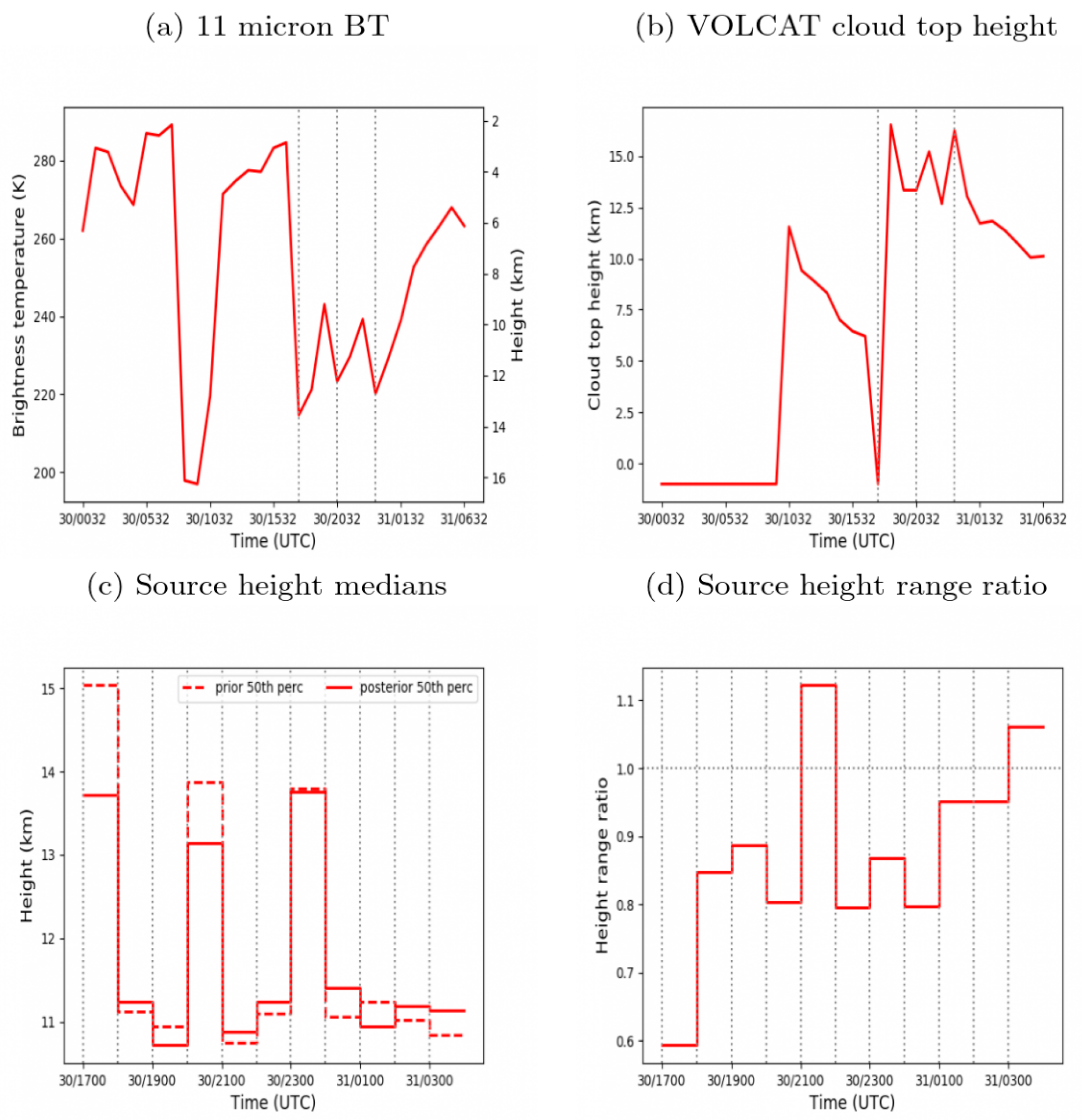
4.1. Source Term
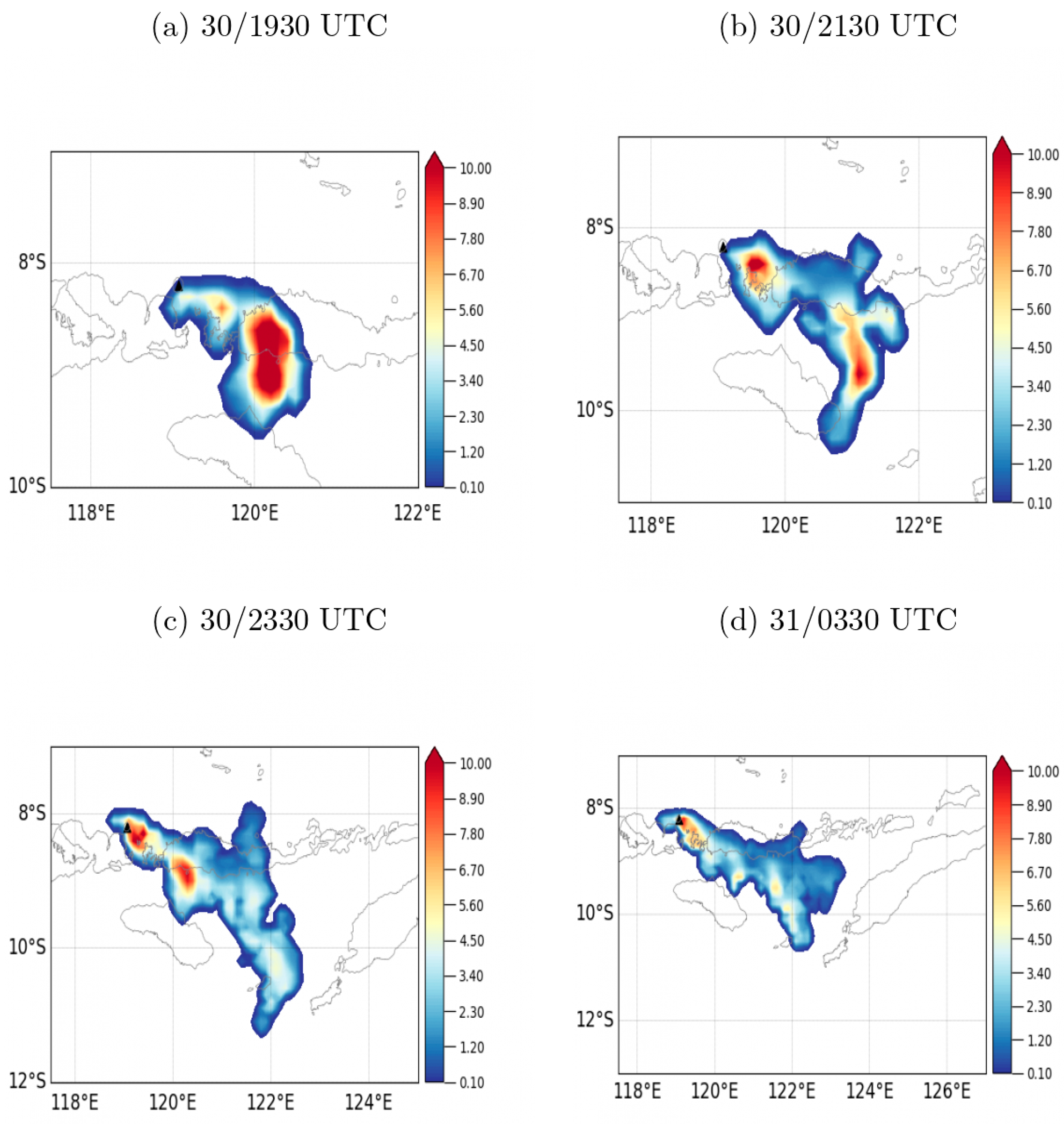
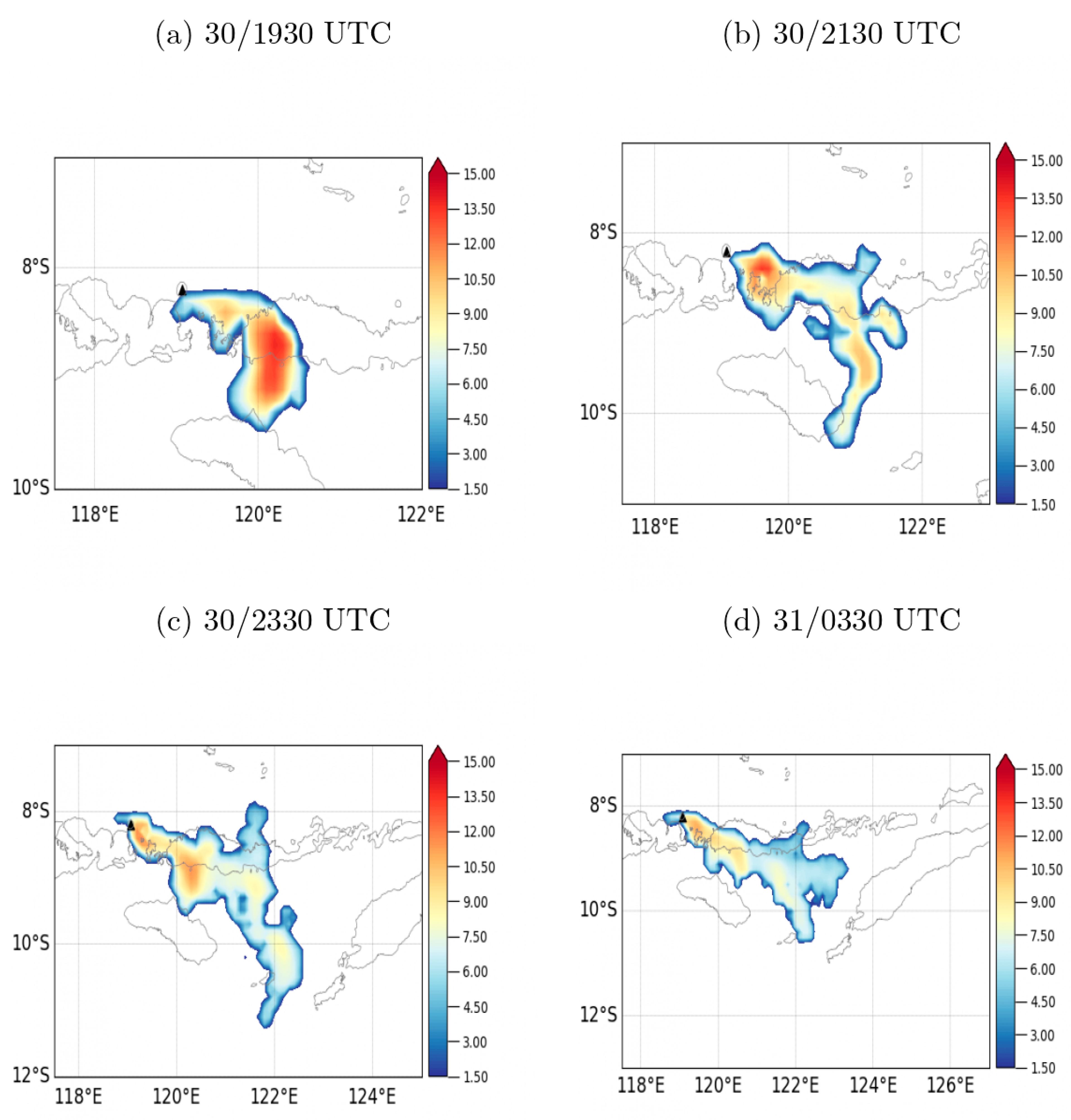
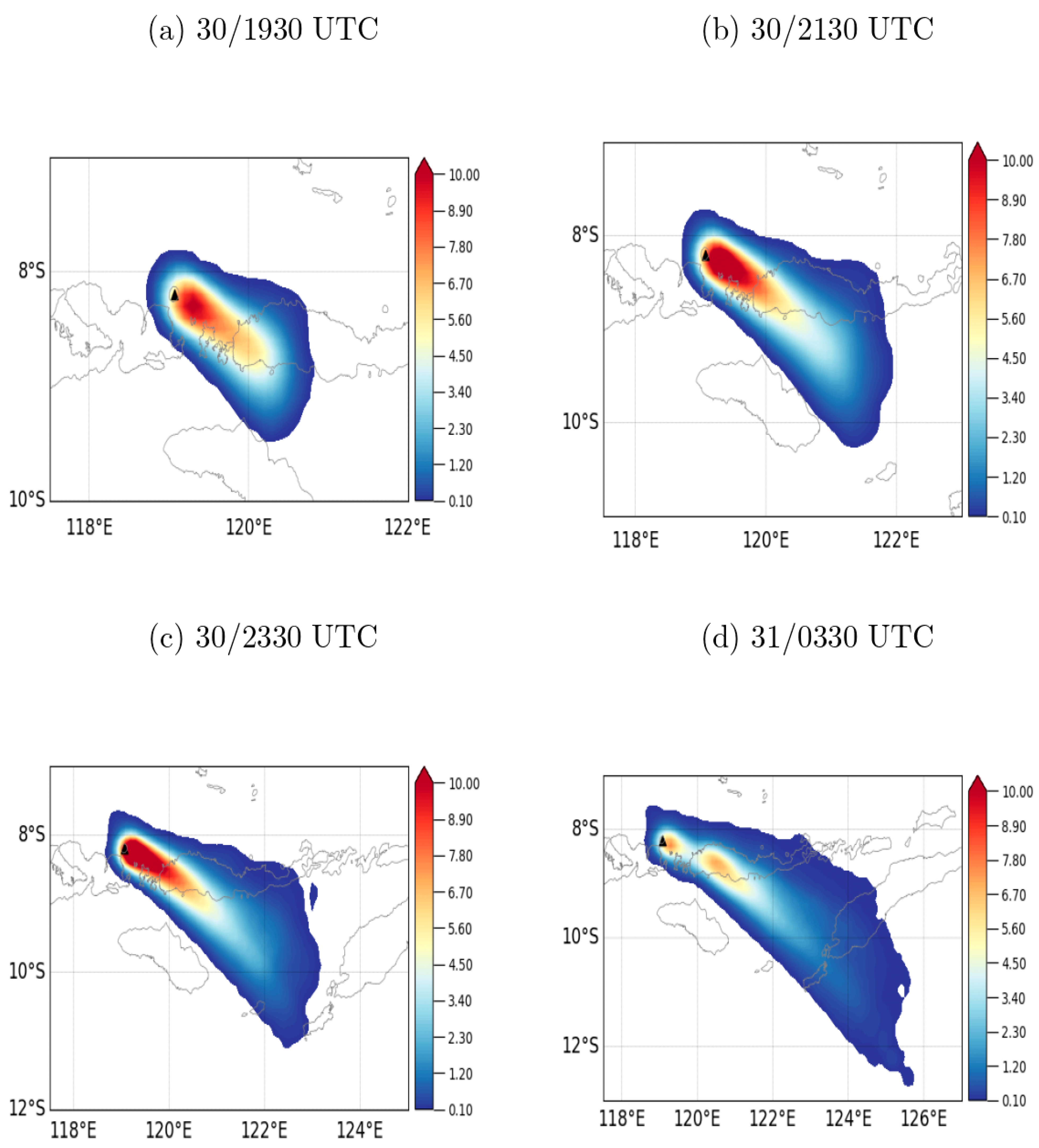
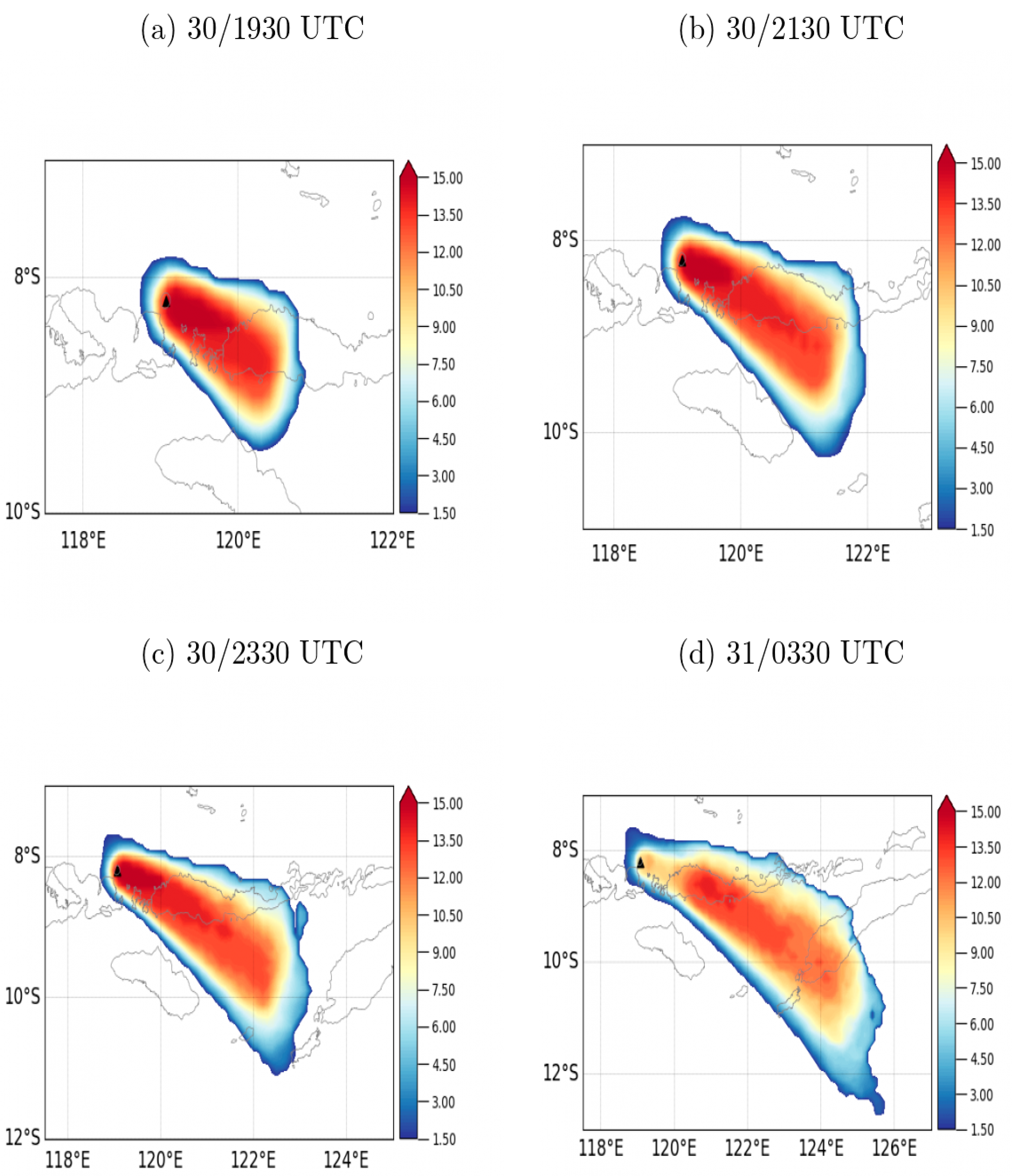
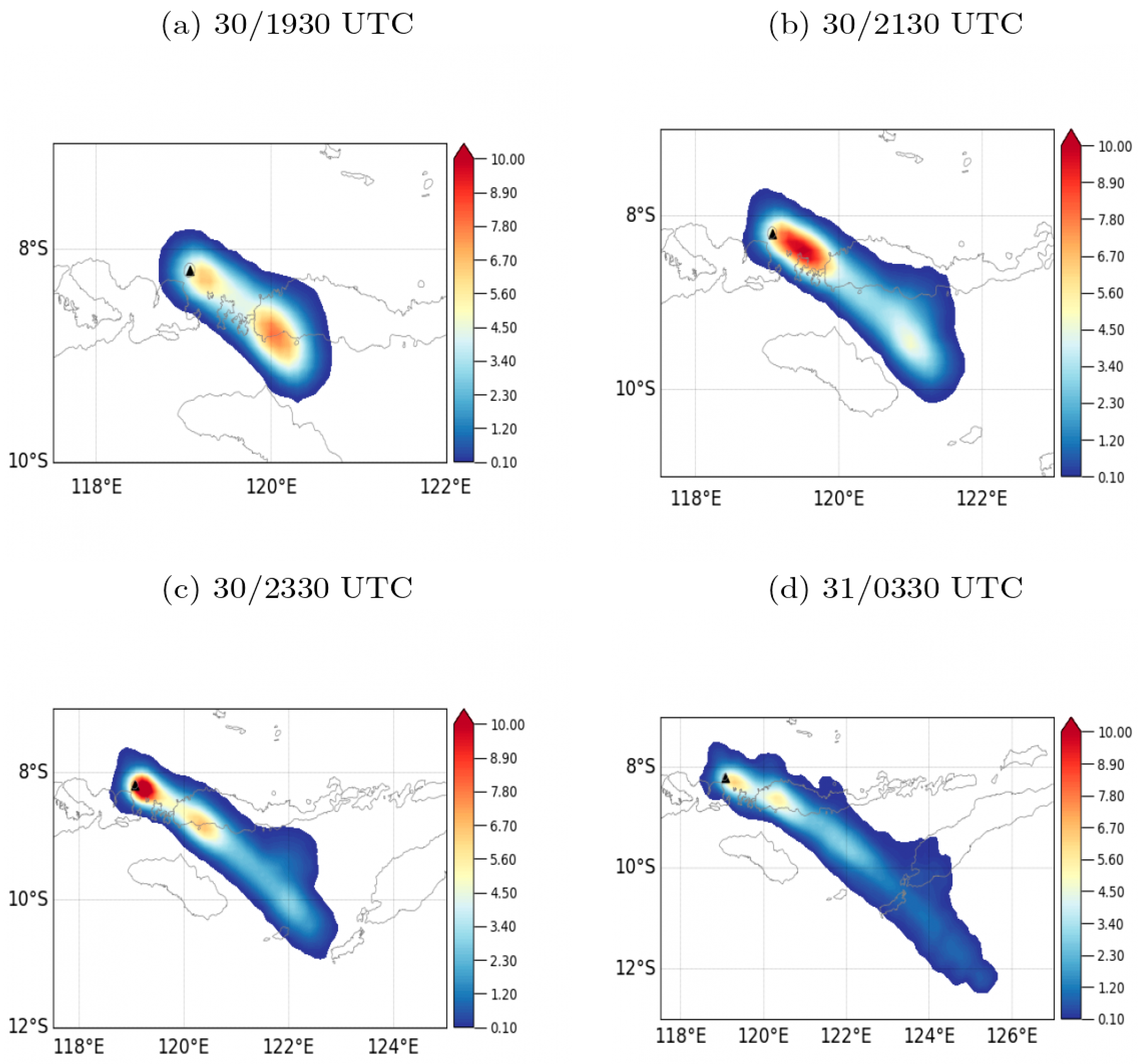
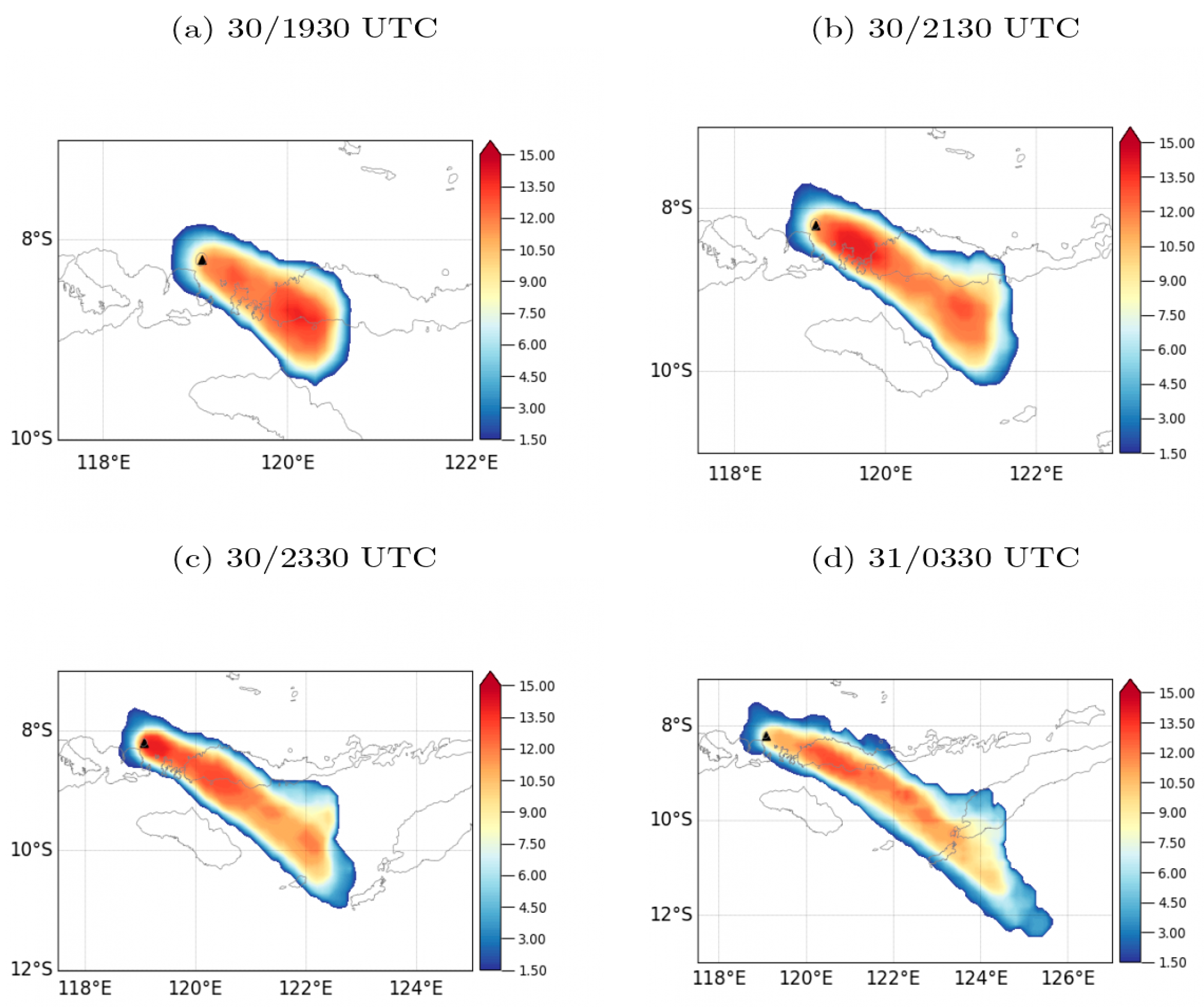
4.2. Ensemble Mean Field Patterns
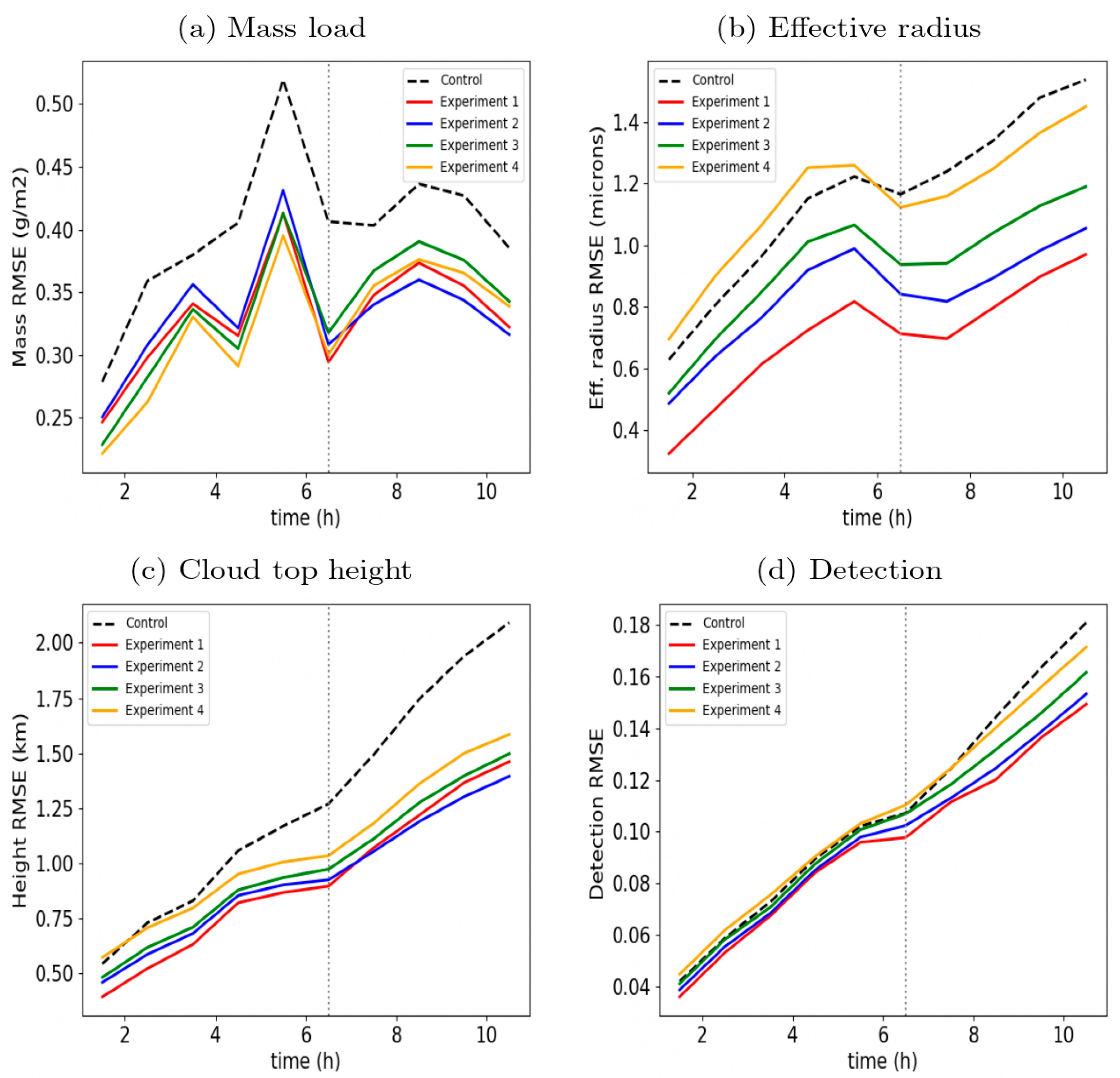
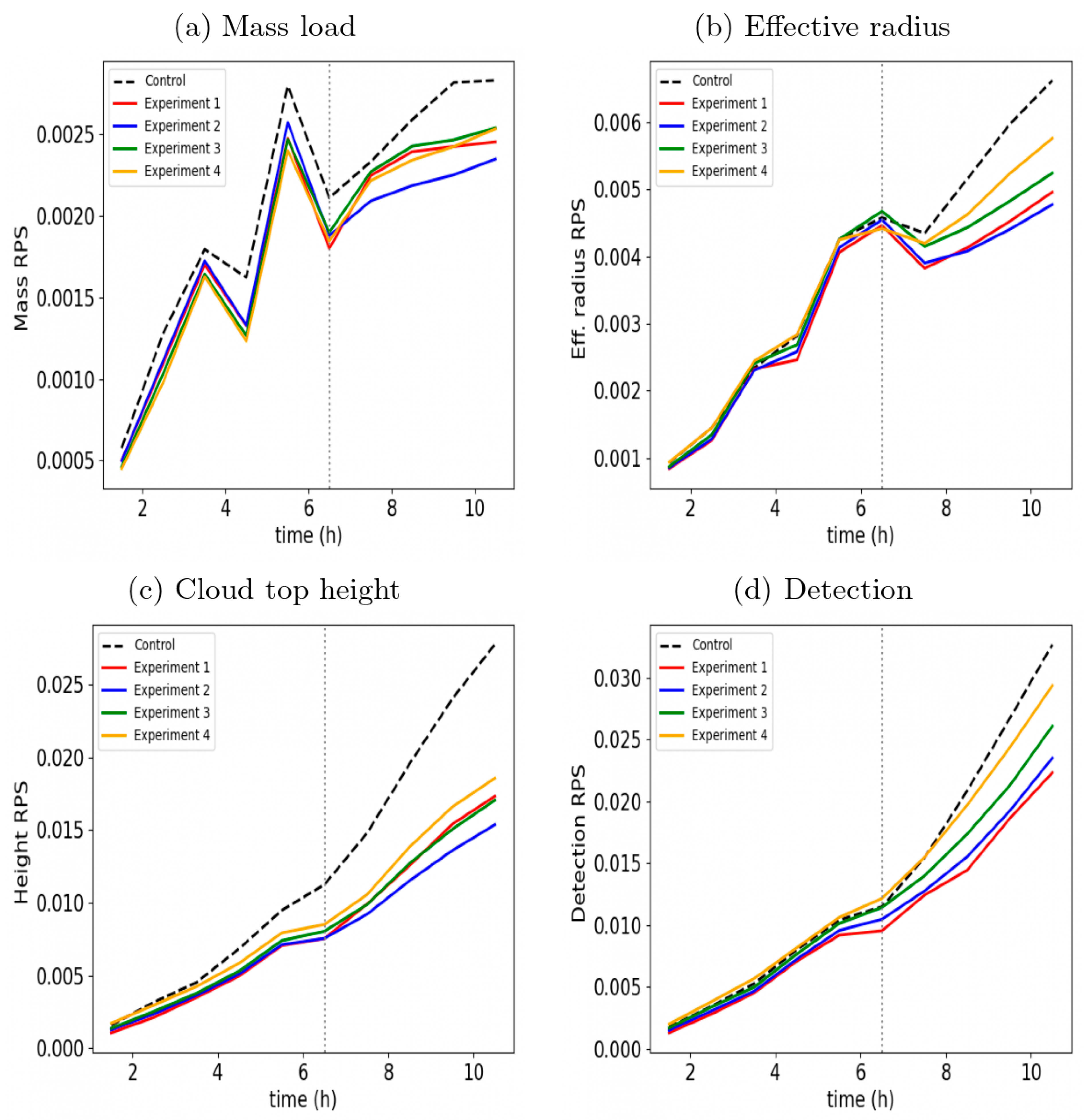
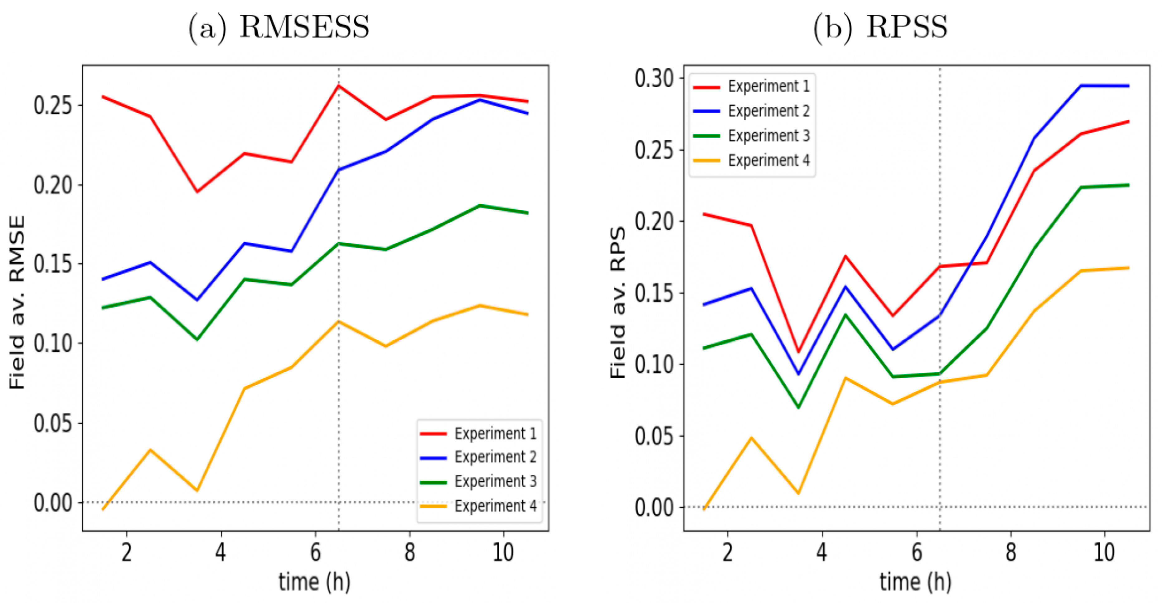
4.3. Verification Study
5. Discussion
6. Conclusions
Funding
Institutional Review Board Statement
Informed Consent Statement
Data Availability Statement
Conflicts of Interest
References
- Casadevall, T.J. Volcanic Ash and Aviation Safety: Proceedings of the First International Symposium on Volcanic Ash and Aviation Safety; DIANE Publishing: Collingdale, PA, USA, 1995; Volume 2047. [Google Scholar]
- O’Kane, T.J.; Naughton, M.J.; Xiao, Y. The Australian community climate and earth system simulator global and regional ensemble prediction scheme. ANZIAM J. 2008, 50, 385–398. [Google Scholar] [CrossRef] [Green Version]
- Bessho, K.; Date, K.; Hayashi, M.; Ikeda, A.; Imai, T.; Inoue, H.; Yoshida, R. An introduction to Himawari-8/9—Japan’s new-generation geostationary meteorological satellites. J. Meteorol. Soc. Jpn. 2016, 94, 151–183. [Google Scholar] [CrossRef] [Green Version]
- Corradini, S.; Merucci, L.; Prata, A.J.; Piscini, A. Volcanic ash and SO2 in the 2008 Kasatochi eruption: Retrievals comparison from different IR satellite sensors. J. Geophys. Res. 2010, 115. [Google Scholar] [CrossRef]
- Francis, P.N.; Cooke, M.C.; Saunders, R.W. Retrieval of physical properties of volcanic ash using Meteosat: A case study from the 2010 Eyjafjallajökull eruption. J. Geophys. Res. 2012, 117. [Google Scholar] [CrossRef]
- Pavolonis, M.J.; Heidinger, A.K.; Sieglaff, J. Automated retrievals of volcanic ash and dust cloud properties from upwelling infrared measurements. J. Geophys. Res. Atmos. 2013, 118, 1436–1458. [Google Scholar] [CrossRef]
- Pavolonis, M.J.; Sieglaff, J.; Cintineo, J. Spectrally Enhanced Cloud Objects—A generalized framework for automated detection of volcanic ash and dust clouds using passive satellite measurements: 1. Multispectral analysis. J. Geophys. Res. Atmos. 2015, 120, 7813–7841. [Google Scholar] [CrossRef]
- Pavolonis, M.J.; Sieglaff, J.; Cintineo, J. Spectrally Enhanced Cloud Objects—A generalized framework for automated detection of volcanic ash and dust clouds using passive satellite measurements: 2. Cloud object analysis and global application. J. Geophys. Res. Atmos. 2015, 120, 7842–7870. [Google Scholar] [CrossRef]
- Eckhardt, S.; Prata, A.J.; Seibert, P.; Stebel, K.; Stohl, A. Estimation of the vertical profile of sulfur dioxide injection into the atmosphere by a volcanic eruption using satellite column measurements and inverse transport modeling. Atmos. Chem. Phys. 2008, 8, 3881–3897. [Google Scholar] [CrossRef] [Green Version]
- Stohl, A.; Prata, A.J.; Eckhardt, S.; Clarisse, L.; Durant, A.; Henne, S. Determination of time-and height-resolved volcanic ash emissions and their use for quantitative ash dispersion modeling: The 2010 Eyjafjallajökull eruption. Atmos. Chem. Phys. 2011, 11, 4333–4351. [Google Scholar] [CrossRef] [Green Version]
- Kristiansen, N.I.; Prata, A.J.; Stohl, A.; Carn, S.A. Stratospheric volcanic ash emissions from the 13 February 2014 Kelut eruption. Geophys. Res. Lett. 2015, 42, 588–596. [Google Scholar] [CrossRef] [Green Version]
- Chai, T.; Crawford, A.; Stunder, B.; Pavolonis, M.J.; Draxler, R.; Stein, A. Improving volcanic ash predictions with the HYSPLIT dispersion model by assimilating MODIS satellite retrievals. Atmos. Chem. Phys. 2017, 17, 2865–2879. [Google Scholar] [CrossRef] [Green Version]
- Harvey, N.J.; Dacre, H.F.; Webster, H.N.; Taylor, I.A.; Khanal, S.; Grainger, R.G.; Cooke, M.C. He impact of ensemble meteorology on inverse modeling estimates of volcano emissions and ash dispersion forecasts: Grímsvötn 2011. Atmosphere 2020, 11, 1022. [Google Scholar] [CrossRef]
- Pelley, R.E.; Thomson, D.J.; Webster, H.N.; Cooke, M.C.; Manning, A.J.; Witham, C.S.; Hort, M.C. A Near-Real-Time Method for Estimating Volcanic Ash Emissions Using Satellite Retrievals. Atmosphere 2021, 12, 1573. [Google Scholar] [CrossRef]
- Mastin, L.G.; Guffanti, M.; Servranckx, R.; Webley, P.; Barsotti, S.; Dean, K. A multidisciplinary effort to assign realistic source parameters to models of volcanic ash-cloud transport and dispersion during eruptions. J. Volcanol. Geotherm. Res. 2009, 186, 10–21. [Google Scholar] [CrossRef]
- Zidikheri, M.J.; Lucas, C. Using satellite data to determine empirical relationships between volcanic ash source parameters. Atmosphere 2020, 11, 342. [Google Scholar] [CrossRef] [Green Version]
- Zidikheri, M.J.; Potts, R.J. A simple inversion method for determining optimal dispersion model parameters from satellite detections of volcanic sulfur dioxide. J. Geophys. Res. Atmos. 2015, 120, 9702–9717. [Google Scholar] [CrossRef]
- Zidikheri, M.J.; Potts, R.; Lucas, C. A probabilistic inverse method for volcanic ash dispersion modelling. ANZIAM J. 2014, 56, 194–209. [Google Scholar] [CrossRef] [Green Version]
- Zidikheri, M.J.; Lucas, C.; Potts, R. Estimation of optimal dispersion model source parameters using satellite detections of volcanic ash. J. Geophys. Res. Atmos. 2017, 122, 8207–8232. [Google Scholar] [CrossRef]
- Zidikheri, M.J.; Lucas, C.; Potts, R.J. Toward quantitative forecasts of volcanic ash dispersal: Using satellite retrievals for optimal estimation of source terms. J. Geophys. Res. Atmos. 2017, 122, 8187–8206. [Google Scholar] [CrossRef]
- Zidikheri, M.J.; Lucas, C.; Potts, R.J. Quantitative verification and calibration of volcanic ash ensemble forecasts using satellite data. J. Geophys. Res. Atmos. 2018, 123, 4135–4156. [Google Scholar] [CrossRef]
- Zidikheri, M.J.; Lucas, C. A computationally efficient ensemble filtering scheme for quantitative volcanic ash forecasts. J. Geophys. Res. Atmos. 2021, 126. [Google Scholar] [CrossRef]
- Zidikheri, M.J.; Lucas, C. Improving Ensemble Volcanic Ash Forecasts by Direct Insertion of Satellite Data and Ensemble Filtering. Atmosphere 2021, 12, 1215. [Google Scholar] [CrossRef]
- Draxler, R.R.; Hess, G.D. An overview of the HYSPLIT_4 modelling system for trajectories. Aust. Meteorol. Mag. 1998, 47, 295–308. [Google Scholar]
- Pavolonis, M.J.; Calvert, C.C.; Cintineo, J.; Sieglaff, J. Transforming satellite data to products in the era of big data. In Adding Value: Applications of Weather and Climate Services-Abstracts of the Eleventh CAWCR Workshop 27 November-1 December 2017, Melbourne, Australia; 2017. Available online: http://www.bom.gov.au/research/publications/cawcrreports/CTR_081.pdf (accessed on 3 August 2022).
- Ohkawara, N. Multifunctional Transport Satellite (MTSAT); Meteorological Satellite Center, Japan Meteorological Agency: Tokyo, Japan, 2003; pp. 1–8. [Google Scholar]


| Field Number (f) | Field Name and Units | Category Number (c) | Threshold Values |
|---|---|---|---|
| 1 | Mass load (g/m2) | 1 | 1.0 |
| 1 | “ | 2 | 10.0 |
| 1 | “ | 3 | 100.0 |
| 1 | “ | 4 | 1000.0 |
| 2 | Effective radius (μm) | 1 | 0.0 |
| 2 | “ | 2 | 5.0 |
| 2 | “ | 3 | 10.0 |
| 2 | “ | 4 | 15.0 |
| 2 | “ | 5 | 20.0 |
| 3 | Cloud top height (km) | 1 | 0.0 |
| 3 | “ | 2 | 5.0 |
| 3 | “ | 3 | 10.0 |
| 3 | “ | 4 | 15.0 |
| 3 | “ | 5 | 20.0 |
| 3 | “ | 6 | 25.0 |
| 4 | Detection (g/m2) | 1 | 0.1 |
| Experiment | |
|---|---|
| 0 (Control) | - |
| 1 | 0.0 |
| 2 | 0.5 |
| 3 | 0.7 |
| 4 | 0.9 |
Publisher’s Note: MDPI stays neutral with regard to jurisdictional claims in published maps and institutional affiliations. |
© 2022 by the author. Licensee MDPI, Basel, Switzerland. This article is an open access article distributed under the terms and conditions of the Creative Commons Attribution (CC BY) license (https://creativecommons.org/licenses/by/4.0/).
Share and Cite
Zidikheri, M.J. Using an Ensemble Filter to Improve the Representation of Temporal Source Variations in a Volcanic Ash Forecasting System. Atmosphere 2022, 13, 1243. https://doi.org/10.3390/atmos13081243
Zidikheri MJ. Using an Ensemble Filter to Improve the Representation of Temporal Source Variations in a Volcanic Ash Forecasting System. Atmosphere. 2022; 13(8):1243. https://doi.org/10.3390/atmos13081243
Chicago/Turabian StyleZidikheri, Meelis J. 2022. "Using an Ensemble Filter to Improve the Representation of Temporal Source Variations in a Volcanic Ash Forecasting System" Atmosphere 13, no. 8: 1243. https://doi.org/10.3390/atmos13081243