
Analysis of MONARC and ACTIVATE Airborne Aerosol Data for Aerosol-Cloud Interaction Investigations: Efficacy of Stairstepping Flight Legs for Airborne In Situ Sampling

 , , , , ,
Abstract
:1. Introduction
2. Methods
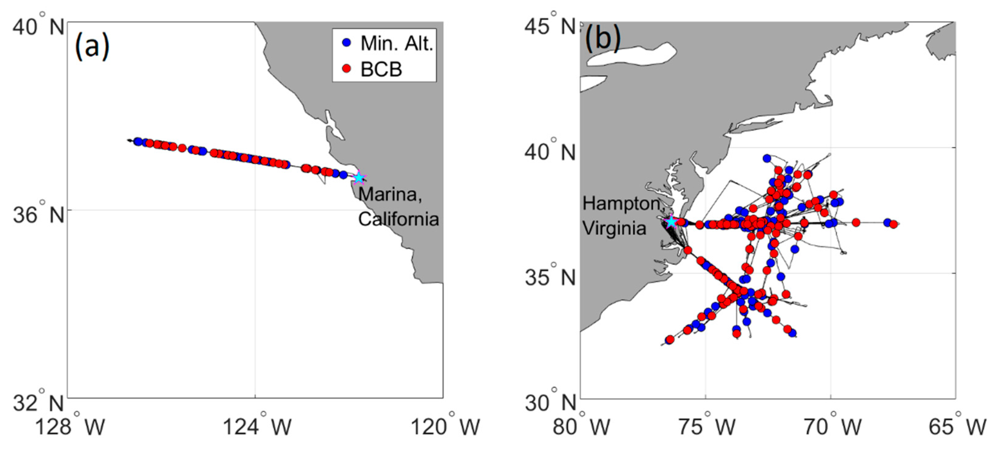
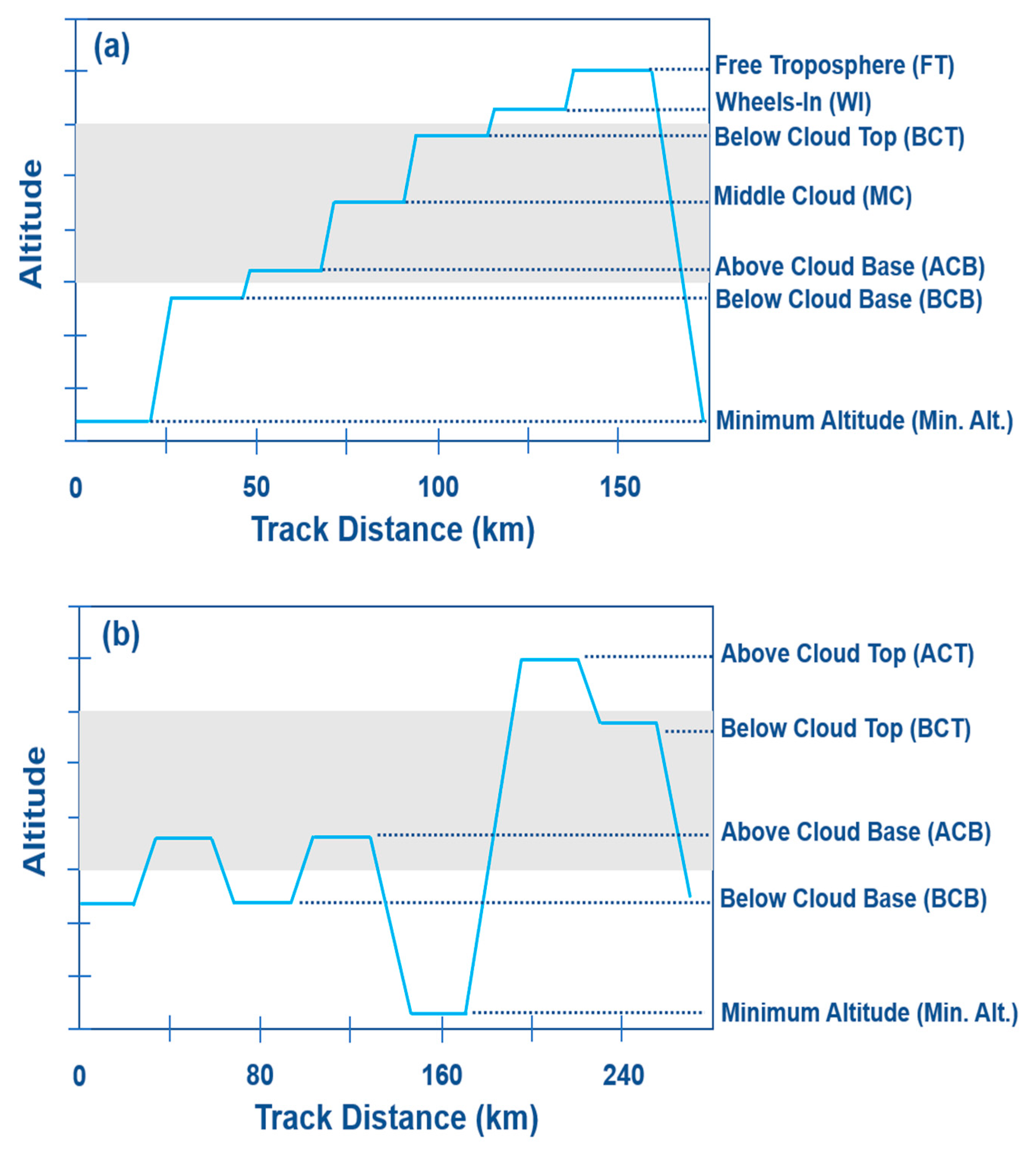
2.1. Field Campaigns and Flight Approach
2.2. Data Variables and Measurements
2.3. Calculations
- Aerosol variables (i.e., measurements provided by CPCs, LAS, PCASP) were screened to remove possible contamination due to the presence of cloud or rain. A strict approach was taken to omit aerosol data in a window of 2 s before and after when either liquid water content or rain water content exceeded 0.005 g m−3.
- In the case of more than one leg (typically 2) flown at the same vertical level in a single ensemble (e.g., two BCB legs in cloud ensembles of ACTIVATE), the one that was closer in distance to the Min. Alt. leg was selected for analyses requiring a comparison of adjacent Min. Alt. and BCB leg data.
- The distance between two legs was calculated based on the distance between the midpoints of the two legs using the great circle equation [22].
- As part of our analysis centers around how well measured values of common variables agree between different legs, statistical analysis was performed. First, linear regressions were performed to assess the degree of correlation between measured variables in two legs. Second, similarity between leg-mean values of specific variables (xi) between two legs was quantified using the mean absolute relative deviation (MARD):where n is the total number of leg pairs examined. MARD is unitless as its normalized by the averages of two legs. For variable values greater than zero, MARD is between 0 and 2 with values closer to 0 associated with more similarity between two legs.
- The standard deviation in horizontal wind speed (σwind) was calculated as a measure of turbulence in the MBL. Higher σwind values indicate more turbulence and likely greater vertical mixing in the MBL. Furthermore, potential temperature (θ) was derived using measurements from Table 1.
3. Results
3.1. Vertical Comparisons
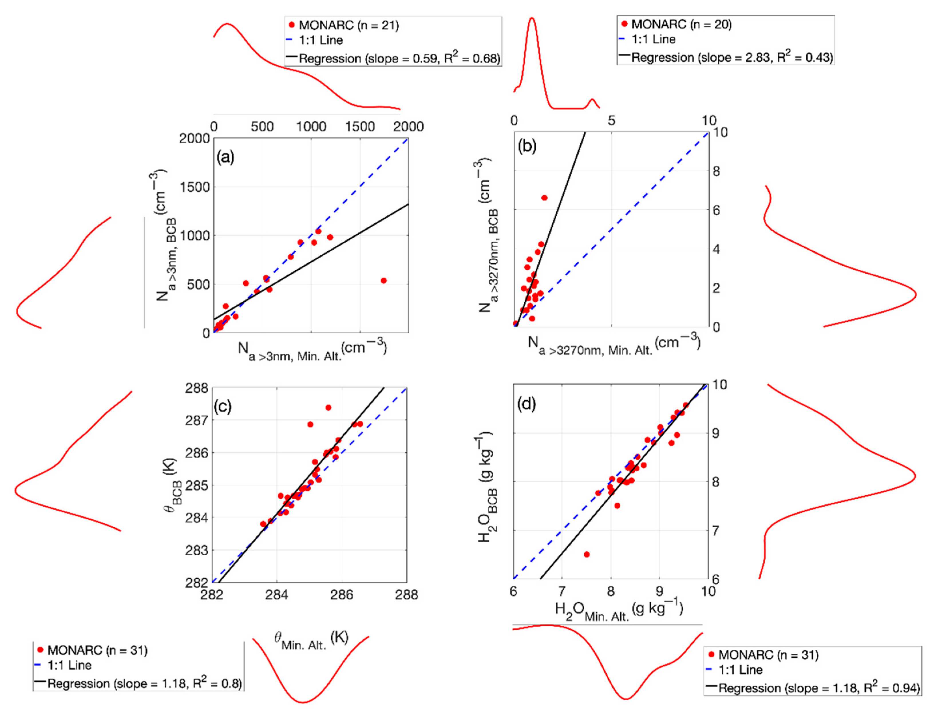
3.1.1. MONARC
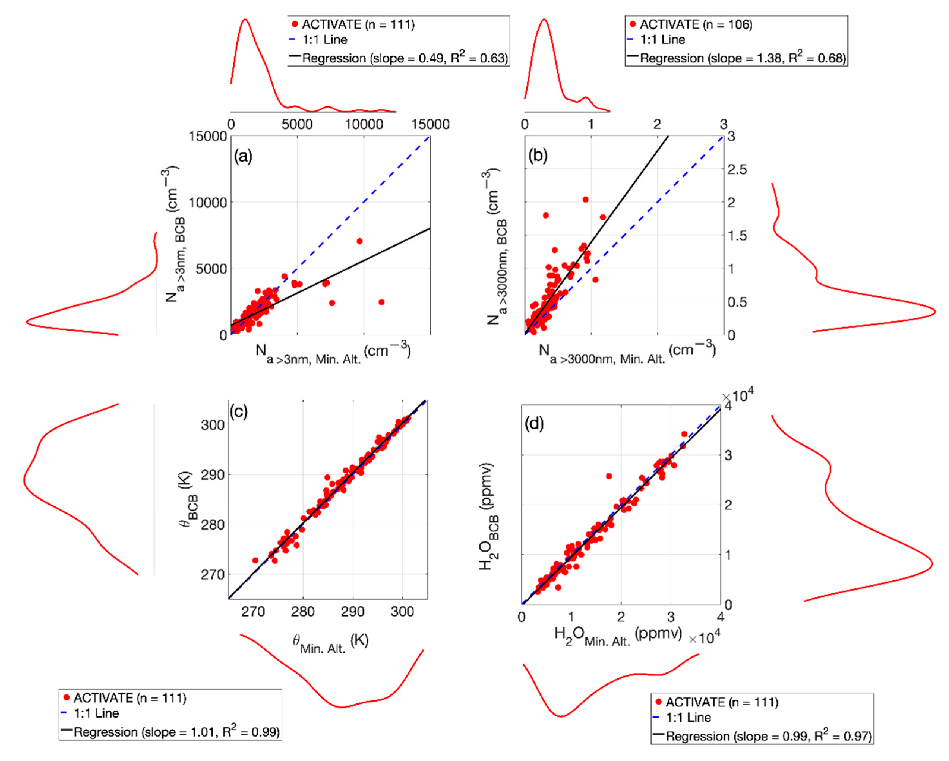
3.1.2. ACTIVATE
3.2. Horizontal Comparisons
4. Case Studies
4.1. Sharp Gradients along Level Legs
4.2. Heterogeneous Cloud Base/Top and Boundary Layer Top Heights
4.3. Poor Vertical Mixing and Multiple Cloud Layers
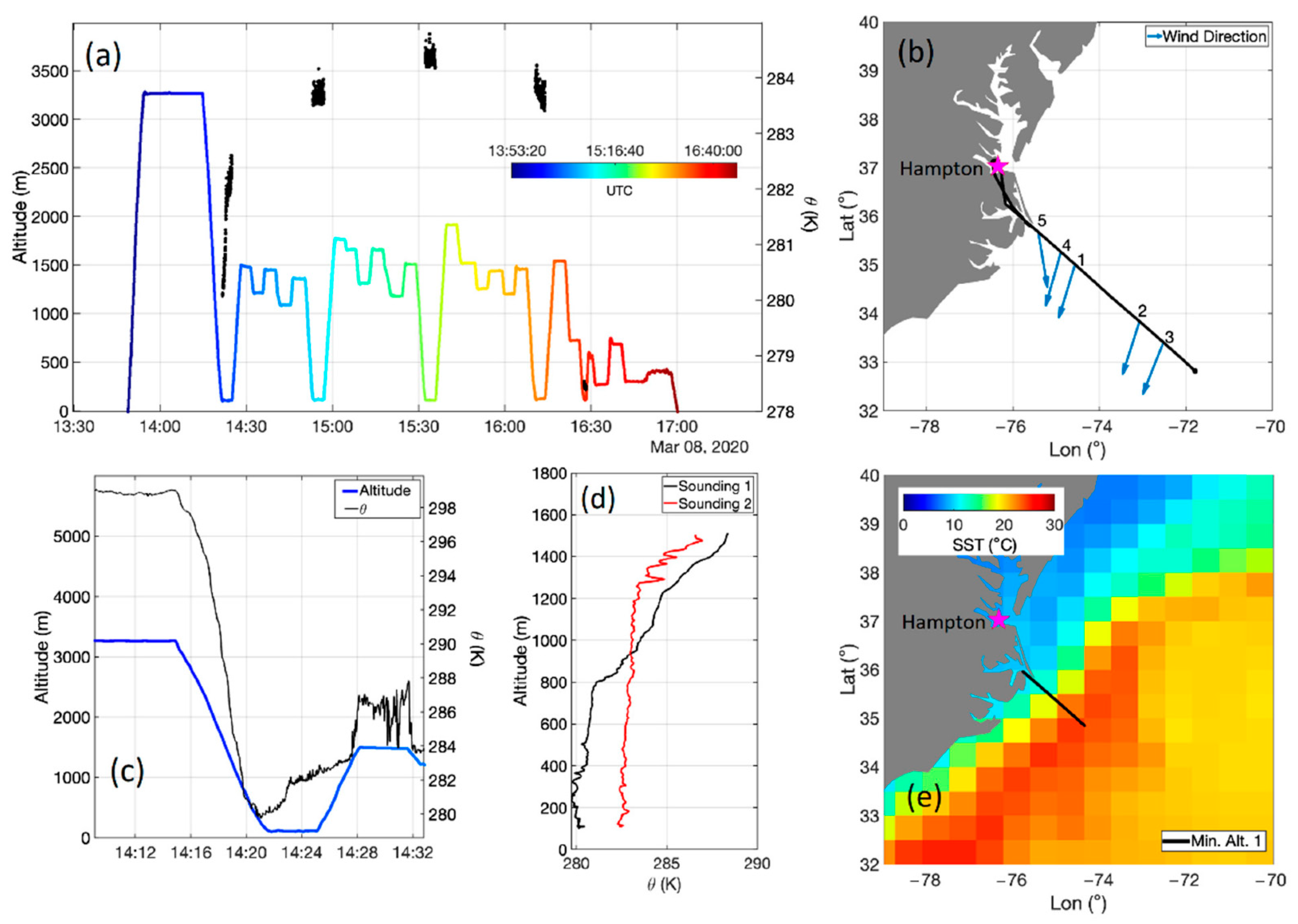
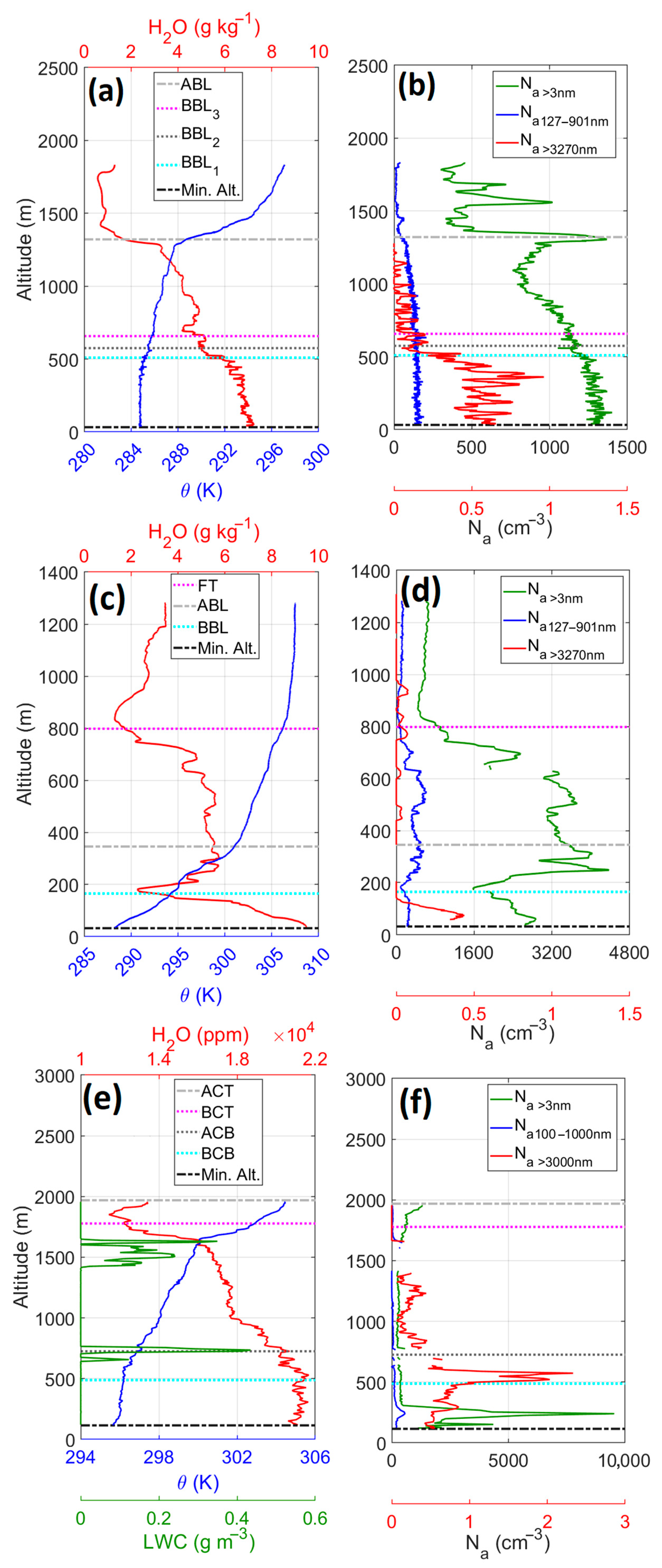
4.3.1. MONARC Research Flight 8 (6 June 2019)
4.3.2. MONARC Research Flight 11 (11 June 2019)
4.3.3. ACTIVATE Research Flight 24 (17 August 2020)
5. Discussion and Conclusions
Supplementary Materials
Author Contributions
Funding
Institutional Review Board Statement
Informed Consent Statement
Data Availability Statement
Acknowledgments
Conflicts of Interest
References
- Mann, J.; Lenschow, D.H. Errors in airborne flux measurements. J. Geophys. Res. Atmos. 1994, 99, 14519–14526. [Google Scholar] [CrossRef]
- Gerber, H.; Frick, G.; Malinowski, S.P.; Jonsson, H.; Khelif, D.; Krueger, S.K. Entrainment rates and microphysics in POST stratocumulus. J. Geophys. Res. Atmos. 2013, 118, 12094–12109. [Google Scholar] [CrossRef]
- Shingler, T.; Crosbie, E.; Ortega, A.; Shiraiwa, M.; Zuend, A.; Beyersdorf, A.; Ziemba, L.; Anderson, B.; Thornhill, L.; Perring, A.E.; et al. Airborne characterization of subsaturated aerosol hygroscopicity and dry refractive index from the surface to 6.5 km during the SEAC4RS campaign. J. Geophys. Res. Atmos. 2016, 121, 4188–4210. [Google Scholar] [CrossRef]
- Chen, Y.C.; Christensen, M.W.; Xue, L.; Sorooshian, A.; Stephens, G.L.; Rasmussen, R.M.; Seinfeld, J.H. Occurrence of lower cloud albedo in ship tracks. Atmos. Chem. Phys. 2012, 12, 8223–8235. [Google Scholar] [CrossRef] [Green Version]
- Albrecht, B.; Ghate, V.; Mohrmann, J.; Wood, R.; Zuidema, P.; Bretherton, C.; Schwartz, C.; Eloranta, E.; Glienke, S.; Donaher, S.; et al. Cloud System Evolution in the Trades (CSET): Following the Evolution of Boundary Layer Cloud Systems with the NSF–NCAR GV. Bull. Am. Meteorol. Soc. 2019, 100, 93–121. [Google Scholar] [CrossRef]
- McFarquhar, G.M.; Bretherton, C.S.; Marchand, R.; Protat, A.; DeMott, P.J.; Alexander, S.P.; Roberts, G.C.; Twohy, C.H.; Toohey, D.; Siems, S.; et al. Observations of Clouds, Aerosols, Precipitation, and Surface Radiation over the Southern Ocean: An Overview of CAPRICORN, MARCUS, MICRE, and SOCRATES. Bull. Am. Meteorol. Soc. 2021, 102, E894–E928. [Google Scholar] [CrossRef]
- Fast, J.D.; Berg, L.K.; Alexander, L.; Bell, D.; D’Ambro, E.; Hubbe, J.; Kuang, C.; Liu, J.; Long, C.; Matthews, A.; et al. Overview of the HI-SCALE Field Campaign: A New Perspective on Shallow Convective Clouds. Bull. Am. Meteorol. Soc. 2019, 100, 821–840. [Google Scholar] [CrossRef] [Green Version]
- Schlosser, J.S.; Dadashazar, H.; Edwards, E.L.; Hossein Mardi, A.; Prabhakar, G.; Stahl, C.; Jonsson, H.H.; Sorooshian, A. Relationships Between Supermicrometer Sea Salt Aerosol and Marine Boundary Layer Conditions: Insights from Repeated Identical Flight Patterns. J. Geophys Res. Atmos 2020, 125, e2019JD032346. [Google Scholar] [CrossRef]
- Sorooshian, A.; Anderson, B.; Bauer, S.E.; Braun, R.A.; Cairns, B.; Crosbie, E.; Dadashazar, H.; Diskin, G.; Ferrare, R.; Flagan, R.C.; et al. Aerosol-cloud–Meteorology Interaction Airborne Field Investigations: Using Lessons Learned from the U.S. West Coast in the Design of ACTIVATE off the U.S. East Coast. Bull. Am. Meteorol. Soc. 2019, 100, 1511–1528. [Google Scholar] [CrossRef] [Green Version]
- Kirschler, S.; Voigt, C.; Anderson, B.; Campos Braga, R.; Chen, G.; Corral, A.F.; Crosbie, E.; Dadashazar, H.; Ferrare, R.A.; Hahn, V.; et al. Seasonal updraft speeds change cloud droplet number concentrations in low-level clouds over the western North Atlantic. Atmos. Chem. Phys. 2022, 22, 8299–8319. [Google Scholar] [CrossRef]
- Lawson, R.P.; O’Connor, D.; Zmarzly, P.; Weaver, K.; Baker, B.; Mo, Q.; Jonsson, H. The 2D-S (Stereo) Probe: Design and Preliminary Tests of a New Airborne, High-Speed, High-Resolution Particle Imaging Probe. J. Atmos. Ocean. Technol. 2006, 23, 1462–1477. [Google Scholar] [CrossRef] [Green Version]
- Dadashazar, H.; Painemal, D.; Alipanah, M.; Brunke, M.; Chellappan, S.; Corral, A.F.; Crosbie, E.; Kirschler, S.; Liu, H.; Moore, R.H.; et al. Cloud drop number concentrations over the western North Atlantic Ocean: Seasonal cycle, aerosol interrelationships, and other influential factors. Atmos. Chem. Phys. 2021, 21, 10499–10526. [Google Scholar] [CrossRef] [PubMed]
- Moore, R.H.; Thornhill, K.L.; Weinzierl, B.; Sauer, D.; D’Ascoli, E.; Kim, J.; Lichtenstern, M.; Scheibe, M.; Beaton, B.; Beyersdorf, A.J.; et al. Biofuel blending reduces particle emissions from aircraft engines at cruise conditions. Nature 2017, 543, 411–415. [Google Scholar] [CrossRef] [PubMed] [Green Version]
- Froyd, K.D.; Murphy, D.M.; Brock, C.A.; Campuzano-Jost, P.; Dibb, J.E.; Jimenez, J.L.; Kupc, A.; Middlebrook, A.M.; Schill, G.P.; Thornhill, K.L.; et al. A new method to quantify mineral dust and other aerosol species from aircraft platforms using single-particle mass spectrometry. Atmos. Meas. Tech. 2019, 12, 6209–6239. [Google Scholar] [CrossRef] [Green Version]
- Knop, I.; Bansmer, S.E.; Hahn, V.; Voigt, C. Comparison of different droplet measurement techniques in the Braunschweig Icing Wind Tunnel. Atmos. Meas. Tech. 2021, 14, 1761–1781. [Google Scholar] [CrossRef]
- Sorooshian, A.; MacDonald, A.B.; Dadashazar, H.; Bates, K.H.; Coggon, M.M.; Craven, J.S.; Crosbie, E.; Hersey, S.P.; Hodas, N.; Lin, J.J.; et al. A multi-year data set on aerosol-cloud-precipitation-meteorology interactions for marine stratocumulus clouds. Sci. Data 2018, 5, 180026. [Google Scholar] [CrossRef] [Green Version]
- DeCarlo, P.F.; Dunlea, E.J.; Kimmel, J.R.; Aiken, A.C.; Sueper, D.; Crounse, J.; Wennberg, P.O.; Emmons, L.; Shinozuka, Y.; Clarke, A.; et al. Fast airborne aerosol size and chemistry measurements above Mexico City and Central Mexico during the MILAGRO campaign. Atmos. Chem. Phys. 2008, 8, 4027–4048. [Google Scholar] [CrossRef] [Green Version]
- Gerber, H.; Arends, B.G.; Ackerman, A.S. New microphysics sensor for aircraft use. Atmos. Res. 1994, 31, 235–252. [Google Scholar] [CrossRef]
- DiGangi, J.P.; Choi, Y.; Nowak, J.B.; Halliday, H.S.; Diskin, G.S.; Feng, S.; Barkley, Z.R.; Lauvaux, T.; Pal, S.; Davis, K.J.; et al. Seasonal Variability in Local Carbon Dioxide Biomass Burning Sources Over Central and Eastern US Using Airborne in Situ Enhancement Ratios. J. Geophys. Res. Atmos. 2021, 126, e2020JD034525. [Google Scholar] [CrossRef]
- Diskin, G.; Podolske, J.; Sachse, G.; Slate, T. Open-Path Airborne Tunable Diode Laser Hygrometer; SPIE: Bellingham, WA, USA, 2002; Volume 4817. [Google Scholar]
- Thornhill, K.L.; Anderson, B.E.; Barrick, J.D.W.; Bagwell, D.R.; Friesen, R.; Lenschow, D.H. Air motion intercomparison flights during Transport and Chemical Evolution in the Pacific (TRACE-P)/ACE-ASIA. J. Geophys. Res. Atmos. 2003, 108. [Google Scholar] [CrossRef] [Green Version]
- Sinnott, R.W. Virtues of the Haversine. In Sky and Telescope; Sky Publishing Corporation: Lincolnshire, IL, USA, 1984; Volume 68, p. 159. [Google Scholar]
- Gonzalez, M.E.; Corral, A.F.; Crosbie, E.; Dadashazar, H.; Diskin, G.S.; Edwards, E.-L.; Kirschler, S.; Moore, R.H.; Robinson, C.E.; Schlosser, J.S.; et al. Relationships between supermicrometer particle concentrations and cloud water sea salt and dust concentrations: Analysis of MONARC and ACTIVATE data. Environ. Sci. Atmos. 2022, 2, 738–752. [Google Scholar] [CrossRef]
- Painemal, D.; Corral, A.F.; Sorooshian, A.; Brunke, M.A.; Chellappan, S.; Afzali Gorooh, V.; Ham, S.-H.; O’Neill, L.; Smith, W.L., Jr.; Tselioudis, G.; et al. An Overview of Atmospheric Features Over the Western North Atlantic Ocean and North American East Coast—Part 2: Circulation, Boundary Layer, and Clouds. J. Geophys. Res. Atmos. 2021, 126, e2020JD033423. [Google Scholar] [CrossRef]
- Corral, A.F.; Choi, Y.; Crosbie, E.; Dadashazar, H.; DiGangi, J.P.; Diskin, G.S.; Fenn, M.; Harper, D.B.; Kirschler, S.; Liu, H.; et al. Cold Air Outbreaks Promote New Particle Formation Off the U.S. East Coast. Geophys. Res. Lett. 2022, 49, e2021GL096073. [Google Scholar] [CrossRef]
- Gelaro, R.; McCarty, W.; Suárez, M.J.; Todling, R.; Molod, A.; Takacs, L.; Randles, C.; Darmenov, A.; Bosilovich, M.G.; Reichle, R.; et al. The Modern-Era Retrospective Analysis for Research and Applications, Version 2 (MERRA-2). J. Clim. 2017, 30, 5419–5454. [Google Scholar] [CrossRef]
- Global Modeling and Assimilation Office (GMAO). Goddard Earth Sciences Data and Information Services Center (GES DISC). Available online: https://disc.gsfc.nasa.gov/ (accessed on 1 June 2022).


| Mission | Variable | Diameter | Instrument | Manufacturer/Reference |
|---|---|---|---|---|
| A/M | Aerosol number concentration (Na>3nm) | >3 nm | Condensation Particle Counter (CPC), model 3776 (A) and 3025 (M) | TSI Inc.; [13] |
| A/M | Aerosol number concentration (Na>10nm) | >10 nm | Condensation Particle Counter (CPC), model 3772 (A) and 3010 (M) | TSI Inc.; [13] |
| A | Aerosol number concentration (Na100–1000nm) | 100–1000 nm | Laser Aerosol Spectrometer (LAS), model 3340 | TSI Inc.; [14] |
| A | Aerosol number concentration (Na>1000nm) | 1–5 μm | Laser Aerosol Spectrometer (LAS), model 3340 | TSI Inc.; [14] |
| A | Aerosol number concentration (Na>3000nm) | 3–50 μm | Fast Cloud Droplet Probe (FCDP) | SPEC Inc.; [15] |
| M | Aerosol number concentration (Na127–901nm) | 127–901 nm | Passive Cavity Aerosol Spectrometer Probe (PCASP) | PMS Inc., modified by DMT Inc.; [16] |
| M | Aerosol number concentration (Na>901nm) | 901–3390 nm | Passive Cavity Aerosol Spectrometer Probe (PCASP) | PMS Inc., modified by DMT Inc.; [16] |
| M | Aerosol number concentration (Na>3270nm) | 3.27–36 μm | Forward Scattering Spectrometer Probe (FSSP) | PMS Inc., modified by DMT Inc.; [16] |
| A | Organic, sulfate mass concentration | <1 μm | High-Resolution Time-of-Flight Aerosol Mass Spectrometer (AMS) | Aerodyne; [17] |
| A | Liquid water content | 3–50 μm | Fast Cloud Droplet Probe | SPEC Inc.; [15] |
| M | Liquid water content | 3–50 μm | Particle Volume Monitor-100A | [18] |
| A | Rain water content | 51.3–1464.9 μm | 2DS Stereo Probe | SPEC Inc.; [11] |
| M | Rain water content | 16–1563 μm | Cloud Imaging Probe | Droplet Measurement Technologies, Inc. |
| A | Methane concentration (CH4) | – | G2401 gas concentration analyzer | PICARRO; [19] |
| A | Carbon dioxide concentration (CO2) | – | G2401 gas concentration analyzer | PICARRO; [19] |
| A | Carbon monoxide concentration (CO) | – | G2401 gas concentration analyzer | PICARRO; [19] |
| A | Ozone concentration (O3) | – | Dual Beam Photometer, Model 205 | PICARRO; [19] |
| A | Water vapor (H2O) | – | Diode Laser Hygrometer (DLH) | [20] |
| M | Water vapor (H2O) | – | Chilled Mirror Hygrometer | EdgeTech Vigilant; [16] |
| A | Horizontal wind speed (Wind) | – | Turbulent Air-Motion Measurement System (TAMMS) | [21] |
| M | Horizontal wind speed (Wind) | – | Five-Hole Radome Gust Probe | [16] |
| (Min. Alt./BCB)/(Min. Alt./BBL) | Cloud/Clear | ||||
|---|---|---|---|---|---|
| Parameter | Median | No. Pairs | Slope | R2 | MARD |
| Altitude (m) | (32/218)/(32/190) | 31/30 | - | - | - |
| Na>3nm (cm−3) | (329/349)/(1041/1035) | 23/26 | 0.59/0.95 | 0.68/0.84 | 0.24/0.18 |
| Na>10nm (cm−3) | (281/292)/(728/802) | 23/26 | 0.64/0.77 | 0.69/0.73 | 0.25/0.24 |
| Na127–901nm (cm−3) | (51/47)/(138/125) | 23/26 | 0.93/0.86 | 0.97/0.83 | 0.26/0.15 |
| Na>901nm (cm−3) | (0.97/0.75)/(2.29/1.85) | 23/26 | 0.63/0.92 | 0.75/0.66 | 0.44/0.35 |
| Na>3270nm (cm−3) | (0.92/1.83)/(0.82/0.76) | 23/26 | 2.83/1.87 | 0.43/0.46 | 0.75/0.50 |
| H2O (g kg−1) | (8.4/8.3)/(7.9/7.2) | 31/30 | 1.18/0.51 | 0.94/0.12 | 0.03/0.14 |
| wind (m s−1) | (11.3/13.0)/(11.8/14.2) | 31/30 | 1.09/1.21 | 0.94/0.84 | 0.10/0.23 |
| σwind (m s−1) | (0.5/0.4)/(0.6/0.5) | 31/30 | 0.57/0.77 | 0.34/0.77 | 0.27/0.32 |
| θ (K) | (284.9/284.9)/(285.2/285.3) | 31/30 | 1.18/1.44 | 0.80/0.93 | 0.00/0.00 |
| (Min. Alt./BCB)/(Min. Alt./BBL) | Cloud (All,Summer,Winter)/Clear (All,Summer,Winter) | ||||
|---|---|---|---|---|---|
| Parameter | Median | No. Pairs | Slope | R2 | MARD |
| Altitude (m) | (118/749)/(119/613) | 111/54 | - | - | - |
| Na>3nm (cm−3) | (1374/1388)/(3022/2617) | 111/54 | (0.49,0.89,0.42)/(1.16,1.28,1.13) | (0.63,0.88,0.59)/(0.57,0.61,0.52) | (0.22,0.15,0.27)/(0.36,0.27,0.43) |
| Na>10nm (cm−3) | (1097/1091)/(2469/2028) | 111/54 | (0.53,0.89,0.46)/(0.98,1.24,0.91) | (0.67,0.88,0.64)/(0.52,0.62,0.47) | (0.22,0.16,0.27)/(0.34,0.27,0.40) |
| Na100–1000nm (cm−3) | (247/258)/(520/513) | 111/54 | (0.90,0.94,0.78)/(0.79,0.81,0.78) | (0.87,0.93,0.70)/(0.76,0.78,0.75) | (0.20,0.15,0.24)/(0.23,0.15,0.29) |
| Na>1000nm (cm−3) | (0.92/0.85)/(0.63/0.53) | 111/54 | (0.91,0.86,1.03)/(0.63,0.65,0.52) | (0.81,0.79,0.70)/(0.60,0.60,0.46) | (0.21,0.20,0.22)/(0.42,0.39,0.44) |
| Na>3000nm (cm−3) | (0.31/0.42)/(0.22/0.14) | 106/48 | (1.38,1.37,1.66)/(0.96,1.36,0.41) | (0.68,0.75,0.43)/(0.47,0.64,0.14) | (0.36,0.33,0.39)/(0.57,0.46,0.63) |
| Organic (μg m−3) | (1.01/0.92)/(2.15/2.36) | 111/53 | (0.95,0.95,0.81)/(0.80,0.69,0.90) | (0.91,0.90,0.78)/(0.84,0.76,0.88) | (0.36,0.40,0.33)/(0.30,0.31,0.29) |
| Sulfate (μg m−3) | (0.81/0.84)/(0.99/1.02) | 111/53 | (0.94,0.88,0.90)/(1.00,0.92,0.86) | (0.86,0.83,0.83)/(0.89,0.83,0.77) | (0.20,0.22,0.19)/(0.19,0.16,0.22) |
| CH4 (ppb) | (1968/1969)/(1988/1986) | 111/54 | (0.95,0.96,0.91)/(0.90,0.98,0.74) | (0.94,0.95,0.87)/(0.82,0.93,0.62) | (0.00,0.00,0.00)/(0.01,0.01,0.01) |
| CO2 (ppm) | (417.7/414.8)/(419.3/418.3) | 111/54 | (0.97,0.91,0.93)/(0.89,0.75,0.52) | (0.97,0.93,0.88)/(0.83,0.77,0.29) | (0.00,0.00,0.00)/(0.01,0.01,0.01) |
| CO (ppb) | (129.2/128.9)/(135.3/137.8) | 111/54 | (0.95,0.97,0.81)/(0.85,1.06,0.63) | (0.95,0.93,0.79)/(0.76,0.92,0.41) | (0.03,0.03,0.02)/(0.06,0.04,0.07) |
| O3 (ppb) | (41.2/41.8)/(45.2/46.0) | 110/54 | (1.02,1.06,0.95)/(1.00,1.04,0.75) | (0.94,0.92,0.89)/(0.80,0.82,0.66) | (0.04,0.06,0.02)/(0.07,0.10,0.04) |
| H2O (ppm) | (11,422/11,351)/(9589/9989) | 111/53 | (0.99,0.99,0.95)/(0.90,0.87,0.80) | (0.97,0.95,0.92)/(0.93,0.82,0.69) | (0.09,0.06,0.11)/(0.23,0.13,0.31) |
| wind (m s−1) | (8.1/7.6)/(6.6/6.4) | 109/54 | (0.99,0.92,1.03)/(0.82,1.02,0.75) | (0.80,0.80,0.81)/(0.48,0.64,0.43) | (0.18,0.13,0.22)/(0.31,0.21,0.38) |
| σwind (m s−1) | (0.7/0.6)/(0.5/0.3) | 111/53 | (0.77,0.70,0.78)/(0.54,0.03,0.63) | (0.71,0.79,0.59)/(0.25,0.00,0.32) | (0.24,0.24,0.24)/(0.55,0.58,0.53) |
| θ (K) | (288.8/289.4)/(286.3/289.9) | 111/54 | (1.01,1.01,1.03)/(0.99,1.20,1.09) | (0.99,0.98,0.96)/(0.97,0.96,0.88) | (0.00,0.00,0.00)/(0.00,0.00,0.01) |
| (Min. Alt./BCB)/(Min. Alt./BBL) | |||
|---|---|---|---|
| Parameter | Slope | Range | Standard Deviation |
| Na>3nm (cm−3) | (2.65/2.53)/(6.14/7.11) | (36/37)/(84/7) | (31/36)/(75/85) |
| Na>10nm (cm−3) | (2.28/2.07)/(4.31/5.60) | (33/29)/(55/6) | (15/17)/(31/20) |
| Na127–901nm (cm−3) | (0.57/0.65)/(0.43/0.44) | (10/9)/(6/0) | (10/10)/(13/13) |
| Na>901nm (cm−3) | (0.0185/0.0258)/(0.0141/0.0184) | (0.25/0.34)/(0.17/0.02) | (1.37/1.35)/(1.53/1.38) |
| Na>3270nm (cm−3) | (0.0181/0.0887)/(0.0055/0.0087) | (0.27/1.19)/(0.08/0.01) | (0.32/0.80)/(0.26/0.26) |
| H2O (g kg−1) | (0.01/0.01)/(0.00/0.01) | (0.1/0.1)/(0.1/0.0) | (0.1/0.1)/(0.1/0.1) |
| wind (m s−1) | (0.022/0.038)/(0.051/0.049) | (0.4/0.6)/(0.6/0.0) | (0.6/0.5)/(0.6/0.6) |
| θ (K) | (0.006/0.008)/(0.006/0.008) | (0.1/0.1)/(0.1/0.0) | (0.1/0.1)/(0.1/0.1) |
| (Min. Alt./BCB)/(Min. Alt./BBL) | |||
|---|---|---|---|
| Parameter | Slope | Range | Standard Deviation |
| Na>3nm (cm−3) | (4.46/4.89)/(18.11/7.68) | (98/112)/(393/176) | (74/87)/(181/138) |
| Na>10nm (cm−3) | (3.46/3.60)/(13.76/6.30) | (80/83)/(307/160) | (37/52)/(102/97) |
| Na100–1000nm (cm−3) | (1.09/1.07)/(1.02/1.73) | (25/24)/(20/47) | (24/28)/(36/38) |
| Na>1000nm (cm−3) | (0.008/0.0091)/(0.0077/0.0074) | (0.19/0.22)/(0.16/0.17) | (0.97/1.00)/(0.88/0.82) |
| Na>3000nm (cm−3) | (0.0021/0.0043)/(0.002/0.0017) | (0.05/0.10)/(0.04/0.04) | (0.13/0.18)/(0.11/0.10) |
| Organic (μg m−3) | (0.0119/0.0112)/(0.0159/0.0164) | (0.27/0.25)/(0.31/0.35) | (0.15/0.18)/(0.14/0.18) |
| Sulfate (μg m−3) | (0.0053/0.0048)/(0.0054/0.0034) | (0.10/0.10)/(0.11/0.08) | (0.05/0.05)/(0.04/0.05) |
| CH4 (ppb) | (0.08/0.06)/(0.17/0.16) | (2/2)/(4/4) | (0/1)/(1/2) |
| CO2 (ppm) | (0.010/0.010)/(0.021/0.015) | (0.2/0.2)/(0.4/0.3) | (0.1/0.1)/(0.1/0.2) |
| CO (ppb) | (0.069/0.062)/(0.099/0.100) | (1.6/1.3)/(2.3/2.5) | (3.1/3.2)/(3.2/3.4) |
| O3 (ppb) | (0.038/0.029)/(0.059/0.036) | (0.8/0.7)/(1.3/0.7) | (1.0/1.1)/(1.0/1.1) |
| H2O (ppm) | (20.22/16.65)/(19.82/34.85) | (453/383)/(395/920) | (261/411)/(256/453) |
| wind (m s−1) | (0.023/0.030)/(0.025/0.030) | (0.5/0.7)/(0.6/0.7) | (1.2/0.8)/(1.3/1.3) |
| θ (K) | (0.009/0.009)/(0.009/0.014) | (0.2/0.2)/(0.2/0.3) | (0.1/0.1)/(0.1/0.1) |
| |Diff.| a | |||
|---|---|---|---|
| Parameter | RF08 (MONARC) | RF11 (MONARC) | RF24 (ACTIVATE) |
| Na>3nm (cm−3) | 220,215,287 | 668 | 39 |
| Na>10nm (cm−3) | 188,186,251 | 432 | 19 |
| Na127–901nm (cm−3) b | 40,40,44 | 74 | 40 |
| Na>3270nm (cm−3) c | 0.18,0.22,0.36 | – | 0.03 |
| H2O (g kg−1) d | 0.9,0.9,2.1 | 5.9 | 275 |
| θ (K) | 0.3,0.3,1.0 | 6.0 | 0.9 |
Publisher’s Note: MDPI stays neutral with regard to jurisdictional claims in published maps and institutional affiliations. |
© 2022 by the authors. Licensee MDPI, Basel, Switzerland. This article is an open access article distributed under the terms and conditions of the Creative Commons Attribution (CC BY) license (https://creativecommons.org/licenses/by/4.0/).
Share and Cite
Dadashazar, H.; Crosbie, E.; Choi, Y.; Corral, A.F.; DiGangi, J.P.; Diskin, G.S.; Dmitrovic, S.; Kirschler, S.; McCauley, K.; Moore, R.H.; et al. Analysis of MONARC and ACTIVATE Airborne Aerosol Data for Aerosol-Cloud Interaction Investigations: Efficacy of Stairstepping Flight Legs for Airborne In Situ Sampling. Atmosphere 2022, 13, 1242. https://doi.org/10.3390/atmos13081242
Dadashazar H, Crosbie E, Choi Y, Corral AF, DiGangi JP, Diskin GS, Dmitrovic S, Kirschler S, McCauley K, Moore RH, et al. Analysis of MONARC and ACTIVATE Airborne Aerosol Data for Aerosol-Cloud Interaction Investigations: Efficacy of Stairstepping Flight Legs for Airborne In Situ Sampling. Atmosphere. 2022; 13(8):1242. https://doi.org/10.3390/atmos13081242
Chicago/Turabian StyleDadashazar, Hossein, Ewan Crosbie, Yonghoon Choi, Andrea F. Corral, Joshua P. DiGangi, Glenn S. Diskin, Sanja Dmitrovic, Simon Kirschler, Kayla McCauley, Richard H. Moore, and et al. 2022. "Analysis of MONARC and ACTIVATE Airborne Aerosol Data for Aerosol-Cloud Interaction Investigations: Efficacy of Stairstepping Flight Legs for Airborne In Situ Sampling" Atmosphere 13, no. 8: 1242. https://doi.org/10.3390/atmos13081242