
Spatio-Temporal Variation of Extreme Heat Events in Southeastern Europe


Abstract
:1. Introduction
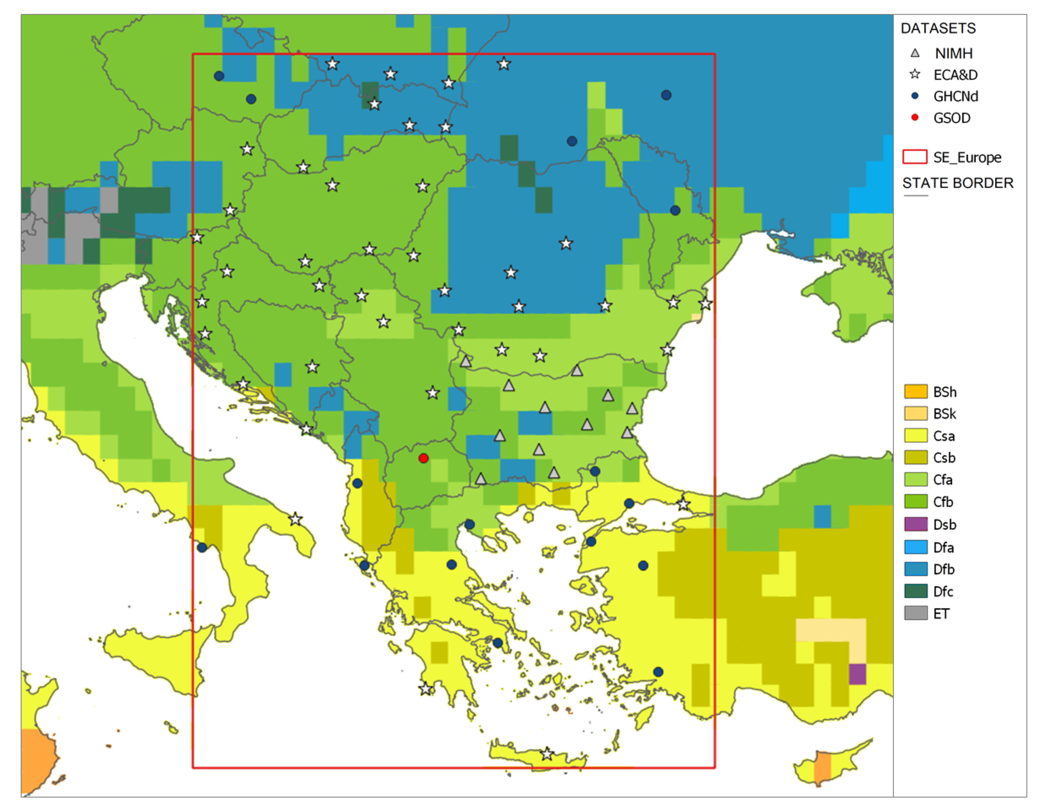
2. Data Sources and Data Pre-Processing
3. Methodology
3.1. Climatologically Justified Threshold Indicators for Bulgaria
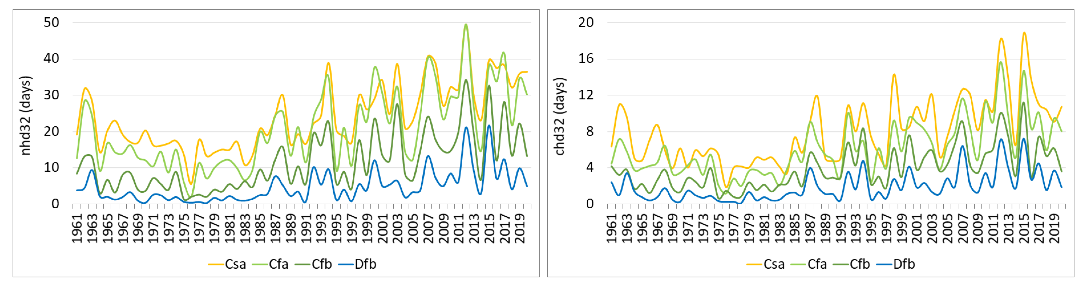
- The annual number of hot days (nhd32)—i.e., the annual count of days when °C.
- The maximum number of consecutive hot days (chd32)—i.e., the longest continuous calendar period when °C.
- The hot spell duration at different thresholds (hsd32/34/36/38/40)—i.e., the annual count of days when , 34, 36, 38, and 40 °C for at least 6, 5, 4, 3, and 2 consecutive days, respectively.
3.2. Excess Heat Factor (EHF)
- −
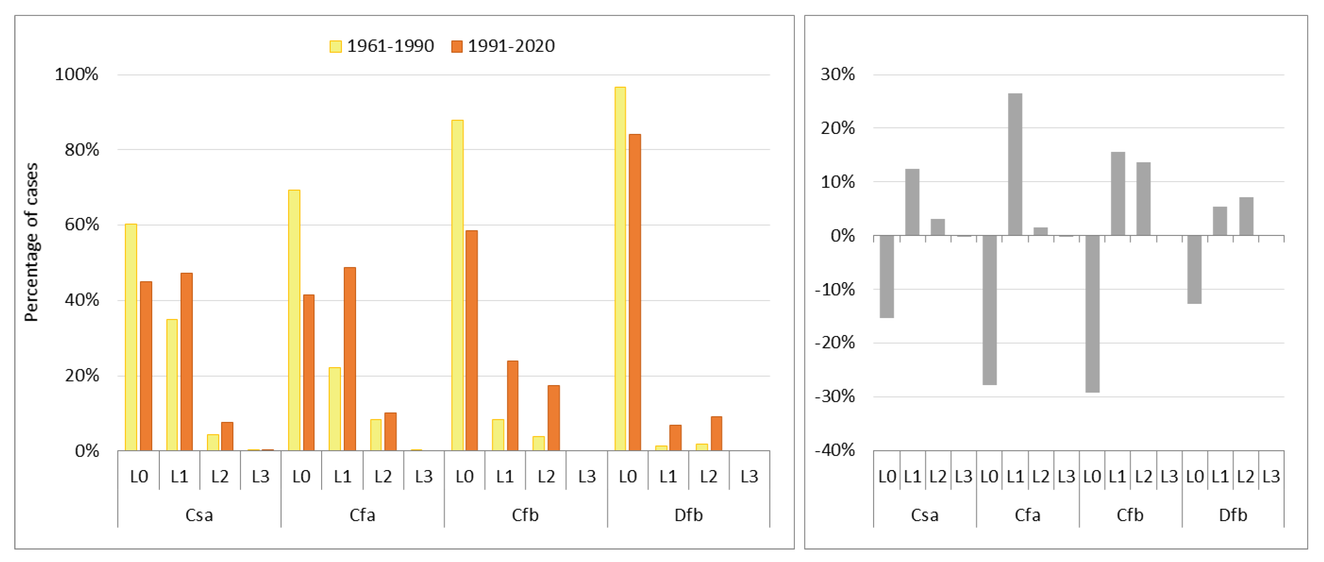
- L1 (low intensity): when ;
- −
- L2 (severe): when ;
- −
- L3 (extreme): when .
3.3. Software Products Used in the Research
4. Results and Discussion
Comparison between EHF Severity and Categories of hsd Indicator
5. Conclusions
Author Contributions
Funding
Institutional Review Board Statement
Informed Consent Statement
Data Availability Statement
Acknowledgments
Conflicts of Interest
Appendix A. Data

| Station ID | Station Name | Country Code (ISO 3166–1) | Latitude (N) | Longitude (E) | Altitude (m) | Data Source | KGC | Environment |
|---|---|---|---|---|---|---|---|---|
| S1 | Belgrade (Obs.) | RS | 44.8 | 20.4667 | 132 | ECA&D | Cfa | urban |
| S2 | Tulcea | RO | 45.1831 | 28.8167 | 4 | ECA&D | Cfa | suburban |
| S3 | Sulina | RO | 45.1667 | 29.7331 | 3 | ECA&D | Cfa | rural |
| S4 | Roşiorii de Vede | RO | 44.1 | 24.9831 | 102 | ECA&D | Cfa | rural |
| S5 | Craiova | RO | 44.23 | 23.87 | 192 | ECA&D | Cfa | rural |
| S6 | Constanţa | RO | 44.22 | 28.63 | 13 | ECA&D | Cfa | suburban |
| S7 | Thessaloniki Airport | GR | 40.52 | 22.97 | 7 | GHCNd | Cfa | airport |
| S8 | Edirne | TR | 41.67 | 26.57 | 51 | GHCNd | Cfa | urban |
| S9 | Sadovo | BG | 42.15 | 24.95 | 155 | NIMH | Cfa | rural |
| S10 | Sandanski | BG | 41.52 | 23.27 | 206 | NIMH | Cfa | suburban |
| S11 | Obraztsov Chiflik | BG | 43.8 | 26.0331 | 156 | NIMH | Cfa | suburban |
| S12 | Goren Chiflik | BG | 43.0094 | 27.6297 | 29 | NIMH | Cfa | suburban |
| S13 | Burgas | BG | 42.4977 | 27.4827 | 22 | NIMH | Cfa | suburban |
| S14 | Kardzhali | BG | 41.65 | 25.37 | 331 | NIMH | Cfa | suburban |
| S15 | Vidin | BG | 43.9942 | 22.8525 | 31 | NIMH | Cfa | suburban |
| S16 | Knezha | BG | 43.5 | 24.0831 | 116 | NIMH | Cfa | rural |
| S17 | Sevlievo | BG | 43.0256 | 25.1151 | 197 | NIMH | Cfa | suburban |
| S18 | Ihtiman | BG | 42.4381 | 23.8196 | 637 | NIMH | Cfb | urban |
| S19 | Shumen | BG | 43.2796 | 26.944 | 217 | NIMH | Cfb | suburban |
| S20 | Sliven | BG | 42.6776 | 26.3398 | 259 | NIMH | Cfb | urban |
| S21 | Zagreb- Grič | HR | 45.8167 | 15.9781 | 156 | ECA&D | Cfb | urban |
| S22 | Budapest | HU | 47.5108 | 19.0206 | 153 | ECA&D | Cfb | urban |
| S23 | Arad | RO | 46.1331 | 21.35 | 116 | ECA&D | Cfb | suburban |
| S24 | Drobeta-Turnu Severin | RO | 44.6331 | 22.6331 | 77 | ECA&D | Cfb | suburban |
| S25 | Hurbanovo | SK | 47.8667 | 18.1831 | 115 | ECA&D | Cfb | suburban |
| S26 | Niš | RS | 43.3331 | 21.9 | 201 | ECA&D | Cfb | suburban |
| S27 | Sarajevo | BA | 43.8678 | 18.4228 | 630 | ECA&D | Cfb | urban |
| S28 | Pécs-Pogány | HU | 46.0056 | 18.2328 | 202 | ECA&D | Cfb | airport |
| S29 | Szeged | HU | 46.2558 | 20.0903 | 81 | ECA&D | Cfb | suburban |
| S30 | Debrecen Airport | HU | 47.4903 | 21.6106 | 107 | ECA&D | Cfb | airport |
| S31 | Gospić | HR | 44.55 | 15.3667 | 564 | ECA&D | Cfb | suburban |
| S32 | Osijek | HR | 45.5331 | 18.6331 | 88 | ECA&D | Cfb | suburban |
| S33 | Novi Sad | RS | 45.3331 | 19.85 | 84 | ECA&D | Cfb | suburban |
| S34 | Šmartno pri Slovenj Gradcu | SI | 46.4894 | 15.1108 | 444 | ECA&D | Cfb | rural |
| S35 | Ogulin | HR | 45.2039 | 15.2717 | 326 | ECA&D | Cfb | rural |
| S36 | Fürstenfeld | AT | 47.0308 | 16.0806 | 323 | ECA&D | Cfb | rural |
| S37 | Gross-Enzersdorf | AT | 48.1994 | 16.5589 | 154 | ECA&D | Cfb | suburban |
| S38 | Kisinev | MD | 47.02 | 28.87 | 173 | GHCNd | Cfb | urban |
| S39 | Přibyslav | CZ | 49.5828 | 15.7625 | 532 | GHCNd | Cfb | rural |
| S40 | Brno-Tuřany | CZ | 49.1531 | 16.6889 | 241 | GHCNd | Cfb | airport |
| S41 | Skopje International Airport | MK | 41.9616 | 21.6214 | 238 | GSOD | Cfb | airport |
| S42 | Heraklion | GR | 35.3331 | 25.1831 | 39 | ECA&D | Csa | airport |
| S43 | Methoni | GR | 36.8331 | 21.7 | 51 | ECA&D | Csa | rural |
| S44 | Brindisi | IT | 40.6331 | 17.9331 | 10 | ECA&D | Csa | urban |
| S45 | Istanbul | TR | 40.9667 | 29.0831 | 33 | ECA&D | Csa | urban |
| S46 | Split Marjan | HR | 43.5167 | 16.4331 | 122 | ECA&D | Csa | urban |
| S47 | Dubrovnik | HR | 42.56 | 18.27 | 52 | ECA&D | Csa | urban |
| S48 | Corfu | GR | 39.62 | 19.92 | 11 | GHCNd | Csa | urban |
| S49 | Hellinikon | GR | 37.9 | 23.75 | 10 | GHCNd | Csa | urban |
| S50 | Cape Palinuro | IT | 40.0251 | 15.2805 | 185 | GHCNd | Csa | rural |
| S51 | Tekirdag | TR | 40.98 | 27.55 | 3 | GHCNd | Csa | urban |
| S52 | Çanakkale | TR | 40.14 | 26.43 | 7 | GHCNd | Csa | airport |
| S53 | Balikesir | TR | 39.62 | 27.93 | 104 | GHCNd | Csa | airport |
| S54 | Larissa | GR | 39.65 | 22.45 | 73 | GHCNd | Csa | airport |
| S55 | Mugla | TR | 37.22 | 28.37 | 646 | GHCNd | Csa | urban |
| S56 | Tirana | AL | 41.3333 | 19.7833 | 38 | GHCNd | Csa | urban |
| S57 | Buzau | RO | 45.1331 | 26.85 | 97 | ECA&D | Dfb | suburban |
| S58 | Poprad-Tatry | SK | 49.0667 | 20.2331 | 694 | ECA&D | Dfb | airport |
| S59 | Sibiu | RO | 45.8 | 24.15 | 444 | ECA&D | Dfb | airport |
| S60 | Bielsko-Białla | PL | 49.8069 | 19.0003 | 396 | ECA&D | Dfb | suburban |
| S61 | Nowy Sa̧cz | PL | 49.6272 | 20.6886 | 292 | ECA&D | Dfb | suburban |
| S62 | Lesko | PL | 49.4664 | 22.3417 | 420 | ECA&D | Dfb | suburban |
| S63 | Miercurea Ciuc | RO | 46.3667 | 25.7331 | 661 | ECA&D | Dfb | rural |
| S64 | Uzhhorod | UA | 48.6331 | 22.2667 | 124 | ECA&D | Dfb | suburban |
| S65 | Caransebeş | RO | 45.42 | 22.25 | 241 | ECA&D | Dfb | airport |
| S66 | Râmnicu Vâlcea | RO | 45.1 | 24.37 | 239 | ECA&D | Dfb | urban |
| S67 | Lviv | UA | 49.8167 | 23.95 | 323 | ECA&D | Dfb | urban |
| S68 | Košice | SK | 48.6667 | 21.2167 | 230 | ECA&D | Dfb | airport |
| S69 | Vinnytsia | UA | 49.23 | 28.6 | 298 | GHCNd | Dfb | airport |
| S70 | Chernivtsi | UA | 48.3667 | 25.9 | 246 | GHCNd | Dfb | rural |

Appendix B. Iterative PCA Imputation Technique Using the R-Package ‘MissMDA’

Appendix C. Defining Hot Spells Duration Indicator (hsd32/34/36/38/40)

Appendix D. Description of EHF Index Calculation
References
- Masson-Delmotte, V.; Zhai, P.; Pirani, A.; Connors, S.; Péan, C.; Berger, S.; Caud, N.; Chen, Y.; Goldfarb, L.; Gomis, M.; et al. Climate Change 2021: The Physical Science Basis. In Contribution of Working Group I to the Sixth Assessment Report of the Intergovernmental Panel on Climate Change; Technical Report; IPCC: Geneva, Switzerland, 2021. [Google Scholar] [CrossRef]
- WMO. State of the Global Climate 2021: WMO Provisional Report; Technical Report; WMO: Geneva, Switzerland, 2021. [Google Scholar]
- Randalls, S. History of the 2 °C climate target. WIREs Clim. Chang. 2010, 1, 598–605. [Google Scholar] [CrossRef]
- Cramer, W.; Guiot, J.; Marini, K. Climate and Environmental Change in the Mediterranean Basin—Current Situation and Risks for the Future; MedECC: First Mediterranean Assessment Report; Technical Report; UNEP/MAP: Marseille, France, 2020. [Google Scholar]
- Vogel, M.M.; Zscheischler, J.; Wartenburger, R.; Dee, D.; Seneviratne, S.I. Concurrent 2018 Hot Extremes Across Northern Hemisphere Due to Human—Induced Climate Change. Earth Future 2019, 7, 692–703. [Google Scholar] [CrossRef] [PubMed]
- Zhang, P.; Jeong, J.H.; Yoon, J.H.; Kim, H.; Wang, S.Y.S.; Linderholm, H.W.; Fang, K.; Wu, X.; Chen, D. Abrupt shift to hotter and drier climate over inner East Asia beyond the tipping point. Science 2020, 370, 1095–1099. [Google Scholar] [CrossRef]
- Diffenbaugh, N.S.; Field, C.B. Changes in Ecologically Critical Terrestrial Climate Conditions. Science 2013, 341, 486–492. [Google Scholar] [CrossRef] [Green Version]
- Vautard, R.; van Aalst, M.; Boucher, O.; Drouin, A.; Haustein, K.; Kreienkamp, F.; van Oldenborgh, G.J.; Otto, F.E.L.; Ribes, A.; Robin, Y.; et al. Human contribution to the record-breaking June and July 2019 heatwaves in Western Europe. Environ. Res. Lett. 2020, 15, 094077. [Google Scholar] [CrossRef]
- WMO. Atlas of Mortality and Economic Losses from Weather, Climate and Water Extremes (1970–2019); Technical Report; WMO: Geneva, Switzerland, 2021. [Google Scholar]
- Sheridan, S.C.; Allen, M.J. Temporal trends in human vulnerability to excessive heat. Environ. Res. Lett. 2018, 13, 043001. [Google Scholar] [CrossRef]
- Petitti, D.B.; Hondula, D.M.; Yang, S.; Harlan, S.L.; Chowell, G. Multiple Trigger Points for Quantifying Heat-Health Impacts: New Evidence from a Hot Climate. Environ. Health Perspect. 2016, 124, 176–183. [Google Scholar] [CrossRef] [PubMed]
- Li, J.; Xu, X.; Yang, J.; Liu, Z.; Xu, L.; Gao, J.; Liu, X.; Wu, H.; Wang, J.; Yu, J.; et al. Ambient high temperature and mortality in Jinan, China: A study of heat thresholds and vulnerable populations. Environ. Res. 2017, 156, 657–664. [Google Scholar] [CrossRef]
- Deryugina, T.; Hsiang, S. Does the Environment Still Matter? Daily Temperature and Income in the United States; Technical Report w20750; National Bureau of Economic Research: Cambridge, MA, USA, 2014. [Google Scholar] [CrossRef]
- García-León, D.; Casanueva, A.; Standardi, G.; Burgstall, A.; Flouris, A.D.; Nybo, L. Current and projected regional economic impacts of heatwaves in Europe. Nat. Commun. 2021, 12, 5807. [Google Scholar] [CrossRef]
- Teixeira, E.I.; Fischer, G.; van Velthuizen, H.; Walter, C.; Ewert, F. Global hot-spots of heat stress on agricultural crops due to climate change. Agric. For. Meteorol. 2013, 170, 206–215. [Google Scholar] [CrossRef]
- Grotjahn, R. Weather Extremes That Affect Various Agricultural Commodities. In Extreme Events and Climate Change, 1st ed.; Castillo, F., Wehner, M., Stone, D.A., Eds.; Wiley: Hoboken, NJ, USA, 2021; pp. 21–48. [Google Scholar] [CrossRef]
- Lass, W.; Haas, A.; Hinkel, J.; Jaeger, C. Avoiding the avoidable: Towards a European heatwaves risk governance. Int. J. Disaster Risk Sci. 2011, 2, 1–14. [Google Scholar] [CrossRef] [Green Version]
- Añel, J.; Fernández-González, M.; Labandeira, X.; López-Otero, X.; de la Torre, L. Impact of Cold Waves and Heat Waves on the Energy Production Sector. Atmosphere 2017, 8, 209. [Google Scholar] [CrossRef] [Green Version]
- Sun, Q.; Miao, C.; Hanel, M.; Borthwick, A.G.; Duan, Q.; Ji, D.; Li, H. Global heat stress on health, wildfires, and agricultural crops under different levels of climate warming. Environ. Int. 2019, 128, 125–136. [Google Scholar] [CrossRef] [PubMed]
- Spinoni, J.; Vogt, J.V.; Barbosa, P.; Dosio, A.; McCormick, N.; Bigano, A.; Füssel, H.M. Changes of heating and cooling degree-days in Europe from 1981 to 2100: HDD and CDD in Europe from 1981 to 2100. Int. J. Climatol. 2018, 38, e191–e208. [Google Scholar] [CrossRef]
- Morabito, M.; Crisci, A.; Messeri, A.; Messeri, G.; Betti, G.; Orlandini, S.; Raschi, A.; Maracchi, G. Increasing Heatwave Hazards in the Southeastern European Union Capitals. Atmosphere 2017, 8, 115. [Google Scholar] [CrossRef] [Green Version]
- Russo, S.; Sillmann, J.; Fischer, E.M. Top ten European heatwaves since 1950 and their occurrence in the coming decades. Environ. Res. Lett. 2015, 10, 124003. [Google Scholar] [CrossRef]
- Beniston, M. The 2003 heat wave in Europe: A shape of things to come? An analysis based on Swiss climatological data and model simulations. Geophys. Res. Lett. 2004, 31. [Google Scholar] [CrossRef] [Green Version]
- Sánchez-Benítez, A.; García-Herera, R.; Barriopedro, D.; Sousa, P.M.; Trigo, R.M. June 2017: The Earliest European Summer Mega-heatwave of Reanalysis Period. Geophys. Res. Lett. 2018, 45, 1955–1962. [Google Scholar] [CrossRef]
- Schär, C.; Vidale, P.L.; Lüthi, D.; Frei, C.; Häberli, C.; Liniger, M.A.; Appenzeller, C. The role of increasing temperature variability in European summer heatwaves. Nature 2004, 427, 332–336. [Google Scholar] [CrossRef]
- Xoplaki, E.; Trigo, R.M.; García-Herera, R.; Barriopedro, D.; D’Andrea, F.; Fischer, E.M.; Gimeno, L.; Gouveia, C.; Hernández, E.; Kuglitsch, F.G.; et al. Large-Scale Atmospheric Circulation Driving Extreme Climate Events in the Mediterranean and its Related Impacts. In The Climate of the Mediterranean Region; Elsevier: Amsterdam, The Netherlands, 2012; pp. 347–417. [Google Scholar] [CrossRef]
- Diffenbaugh, N.S.; Pal, J.S.; Giorgi, F.; Gao, X. Heat stress intensification in the Mediterranean climate change hotspot. Geophys. Res. Lett. 2007, 34, L11706. [Google Scholar] [CrossRef] [Green Version]
- Della-Marta, P.M.; Luterbacher, J.; von Weissenfluh, H.; Xoplaki, E.; Brunet, M.; Wanner, H. Summer heatwaves over western Europe 1880–2003, their relationship to large-scale forcings and predictability. Clim. Dyn. 2007, 29, 251–275. [Google Scholar] [CrossRef] [Green Version]
- Kuglitsch, F.G.; Toreti, A.; Xoplaki, E.; Della-Marta, P.M.; Zerefos, C.S.; Türkeş, M.; Luterbacher, J. Heat wave changes in the eastern Mediterranean since 1960. Geophys. Res. Lett. 2010, 37. [Google Scholar] [CrossRef] [Green Version]
- Tolika, K. Assessing Heat Waves over Greece Using the Excess Heat Factor (EHF). Climate 2019, 7, 9. [Google Scholar] [CrossRef] [Green Version]
- Horton, R.M.; Mankin, J.S.; Lesk, C.; Coffel, E.; Raymond, C. A Review of Recent Advances in Research on Extreme Heat Events. Curr. Clim. Chang. Rep. 2016, 2, 242–259. [Google Scholar] [CrossRef]
- Kottek, M.; Grieser, J.; Beck, C.; Rudolf, B.; Rubel, F. World Map of the Köppen-Geiger climate classification updated. Meteorol. Z. 2006, 15, 259–263. [Google Scholar] [CrossRef]
- Lionello, P.; Abrantes, F.; Congedi, L.; Dulac, F.; Gacic, M.; Gomis, D.; Goodess, C.; Hoff, H.; Kutiel, H.; Luterbacher, J.; et al. Introduction: Mediterranean Climate–Background Information. In The Climate of the Mediterranean Region; Elsevier: Amsterdam, The Netherlands, 2012. [Google Scholar] [CrossRef] [Green Version]
- Perkins, S.E. A review on the scientific understanding of heatwaves—Their measurement, driving mechanisms, and changes at the global scale. Atmos. Res. 2015, 164–165, 242–267. [Google Scholar] [CrossRef]
- Russo, S.; Dosio, A.; Graversen, R.G.; Sillmann, J.; Carrao, H.; Dunbar, M.B.; Singleton, A.; Montagna, P.; Barbola, P.; Vogt, J.V. Magnitude of extreme heatwaves in present climate and their projection in a warming world. J. Geophys. Res. Atmos. 2014, 119, 12500–12512. [Google Scholar] [CrossRef] [Green Version]
- Perkins, S.E.; Alexander, L.V. On the Measurement of Heat Waves. J. Clim. 2013, 26, 4500–4517. [Google Scholar] [CrossRef]
- Nairn, J.; Ostendorf, B.; Bi, P. Performance of Excess Heat Factor Severity as a Global Heatwave Health Impact Index. Int. J. Environ. Res. Public Health 2018, 15, 2494. [Google Scholar] [CrossRef] [Green Version]
- Casanueva, A.; Burgstall, A.; Kotlarski, S.; Messeri, A.; Morabito, M.; Flouris, A.D.; Nybo, L.; Spirig, C.; Schwierz, C. Overview of Existing Heat-Health Warning Systems in Europe. Int. J. Environ. Res. Public Health 2019, 16, 2657. [Google Scholar] [CrossRef] [Green Version]
- Tong, S.; Wang, X.Y.; Barnett, A.G. Assessment of Heat-Related Health Impacts in Brisbane, Australia: Comparison of Different Heatwave Definitions. PLoS ONE 2010, 5, e12155. [Google Scholar] [CrossRef] [Green Version]
- Sulikowska, A.; Wypych, A. Summer temperature extremes in Europe: How does the definition affect the results? Theor. Appl. Climatol. 2020, 141, 19–30. [Google Scholar] [CrossRef] [Green Version]
- Di Napoli, C.; Pappenberger, F.; Cloke, H.L. Assessing heat-related health risk in Europe via the Universal Thermal Climate Index (UTCI). Int. J. Biometeorol. 2018, 62, 1155–1165. [Google Scholar] [CrossRef] [Green Version]
- Matzarakis, A.; Laschewski, G.; Muthers, S. The Heat Health Warning System in Germany-Application and Warnings for 2005 to 2019. Atmosphere 2020, 11, 170. [Google Scholar] [CrossRef] [Green Version]
- Dunn, R.J.H.; Alexander, L.V.; Donat, M.G.; Zhang, X.; Bador, M.; Herold, N.; Lippmann, T.; Allan, R.; Aguilar, E.; Barry, A.A.; et al. Development of an Updated Global Land In Situ-Based Data Set of Temperature and Precipitation Extremes: HadEX3. J. Geophys. Res. Atmos. 2020, 125, e2019JD032263. [Google Scholar] [CrossRef]
- Donat, M.; Alexander, L.; Yang, H.; Durre, I.; Vose, R.; Caesar, J. Global Land-Based Datasets for Monitoring Climatic Extremes. Bull. Am. Meteorol. Soc. 2013, 94, 997–1006. [Google Scholar] [CrossRef] [Green Version]
- Di Napoli, C.; Barnard, C.; Prudhomme, C.; Cloke, H.L.; Pappenberger, F. ERA5-HEAT: A global gridded historical dataset of human thermal comfort indices from climate reanalysis. Geosci. Data J. 2021, 8, 2–10. [Google Scholar] [CrossRef]
- Raei, E.; Nikoo, M.R.; AghaKouchak, A.; Mazdiyasni, O.; Sadegh, M. GHWR, a multi-method global heatwave and warm-spell record and toolbox. Sci. Data 2018, 5, 180206. [Google Scholar] [CrossRef]
- Domínguez-Castro, F.; Reig, F.; Vicente-Serrano, S.M.; Aguilar, E.; Peña-Angulo, D.; Noguera, I.; Revuelto, J.; van der Schrier, G.; El Kenawy, A.M. A multidecadal assessment of climate indices over Europe. Sci. Data 2020, 7, 125. [Google Scholar] [CrossRef]
- Chervenkov, H.; Slavov, K.; Ivanov, V. STARDEX and ETCCDI climate indices based on E-OBS and CARPATCLIM part one: General description. In Numerical Methods and Applications; Nikolov, G., Kolkovska, N., Georgiev, K., Eds.; Springer: Cham, Switzerland, 2019; Volume 11189, pp. 360–367. [Google Scholar]
- Urban, A.; Kyselý, J. Comparison of UTCI with other thermal indices in the assessment of heat and cold effects on cardiovascular mortality in the Czech Republic. Int. J. Environ. Res. Public Health 2014, 11, 952–967. [Google Scholar] [CrossRef] [Green Version]
- Founda, D.; Giannakopoulos, C. The exceptionally hot summer of 2007 in Athens, Greece—A typical summer in the future climate? Glob. Planet. Chang. 2009, 67, 227–236. [Google Scholar] [CrossRef]
- Pecelj, M.M.; Lukić, M.Z.; Filipović, D.J.; Protić, B.M.; Bogdanović, U.M. Analysis of the universal thermal climate index during heatwaves in Serbia. Nat. Hazards Earth Syst. Sci. 2020, 20, 2021–2036. [Google Scholar] [CrossRef]
- Urban, A.; Hanzlíková, H.; Kyselý, J.; Plavcová, E. Impacts of the 2015 heatwaves on mortality in the Czech Republic—A comparison with previous heatwaves. Int. J. Environ. Res. Public Health 2017, 14, 1562. [Google Scholar] [CrossRef] [Green Version]
- Piticar, A.; Croitoru, A.E.; Ciupertea, F.A.; Harpa, G.V. Recent changes in heatwaves and cold waves detected based on excess heat factor and excess cold factor in Romania: Changes in heat wave and cold wave indices in Romania. Int. J. Climatol. 2018, 38, 1777–1793. [Google Scholar] [CrossRef]
- Katavoutas, G.; Founda, D. Response of urban heat stress to heatwaves in Athens (1960–2017). Atmosphere 2019, 10, 483. [Google Scholar] [CrossRef] [Green Version]
- Gocheva, A.; Malcheva, K. Extremely hot spells on the territory of Bulgaria. Bulg. J. Meteorol. Hydrol. 2010, 15, 64–81. [Google Scholar]
- Malcheva, K.; Bocheva, L.; Chervenkov, H. Climatology of extremely hot spells in Bulgaria (1961–2019). In Proceedings of the 21st International Multidisciplinary Scientific GeoConference SGEM 2021, STEF92 Technology, Sofia, Bulgaria, 16–22 August 2021; Trofymchuk, O., Rivza, B., Eds.; Volume 21, pp. 237–244. [Google Scholar] [CrossRef]
- Klein Tank, A.M.G.; Wijngaard, J.B.; Können, G.P.; Böhm, R.; Demarée, G.; Gocheva, A.; Mileta, M.; Pashiardis, S.; Hejkrlik, L.; Kern-Hansen, C.; et al. Daily dataset of 20th-century surface air temperature and precipitation series for the European Climate Assessment. Int. J. Climatol. 2002, 22, 1441–1453. [Google Scholar] [CrossRef]
- Menne, M.J.; Durre, I.; Vose, R.S.; Gleason, B.E.; Houston, T.G. An Overview of the Global Historical Climatology Network-Daily Database. J. Atmos. Ocean. Technol. 2012, 29, 897–910. [Google Scholar] [CrossRef]
- H Sparks, A.; Hengl, T.; Nelson, A. GSODR: Global Summary Daily Weather Data in R. J. Open Source Softw. 2017, 2, 177. [Google Scholar] [CrossRef]
- Morabito, M.; Messeri, A.; Noti, P.; Casanueva, A.; Crisci, A.; Kotlarski, S.; Orlandini, S.; Schwierz, C.; Spirig, C.; Kingma, B.R.; et al. An Occupational Heat-Health Warning System for Europe: The HEAT-SHIELD Platform. Int. J. Environ. Res. Public Health 2019, 16, 2890. [Google Scholar] [CrossRef] [Green Version]
- Alexander, L.V.; Zhang, X.; Peterson, T.C.; Caesar, J.; Gleason, B.; Klein Tank, A.M.G.; Haylock, M.; Collins, D.; Trewin, B.; Rahimzadeh, F.; et al. Global observed changes in daily climate extremes of temperature and precipitation. J. Geophys. Res. 2006, 111, D05109. [Google Scholar] [CrossRef] [Green Version]
- Caesar, J.; Alexander, L.; Vose, R. Large-scale changes in observed daily maximum and minimum temperatures: Creation and analysis of a new gridded data set. J. Geophys. Res. 2006, 111, D05101. [Google Scholar] [CrossRef]
- Wijngaard, J.B.; Klein Tank, A.M.G.; Können, G.P. Homogeneity of 20th century European daily temperature and precipitation series: Homogeneity of European Climate Series. Int. J. Climatol. 2003, 23, 679–692. [Google Scholar] [CrossRef]
- Durre, I.; Menne, M.J.; Gleason, B.E.; Houston, T.G.; Vose, R.S. Comprehensive Automated Quality Assurance of Daily Surface Observations. J. Appl. Meteorol. Climatol. 2010, 49, 1615–1633. [Google Scholar] [CrossRef] [Green Version]
- Josse, J.; Husson, F. MissMDA: A Package for Handling Missing Values in Multivariate Data Analysis. J. Stat. Softw. 2016, 70, 1–31. [Google Scholar] [CrossRef]
- Tveito, O.E.; Aṇiskeviča, S.; Cappelen, J.; Engström, E.; Gjelten, H.M.; Jensen, C.D.; Jokinen, P.; Kuya, E.K.; Lussana, C.; Mäkelä, A.; et al. ClimNorm—Temperature Data Set, Gap Filling Methods and Regional Analysis to Prepare New Climate Normals; MET Report 04/2020; Norwegian Meteorological Institute: Oslo, Norway, 2020. [Google Scholar]
- Muñoz-Sabater, J.; Dutra, E.; Agustí-Panareda, A.; Albergel, C.; Arduini, G.; Balsamo, G.; Boussetta, S.; Choulga, M.; Harrigan, S.; Hersbach, H.; et al. ERA5-Land: A state-of-the-art global reanalysis dataset for land applications. Earth Syst. Sci. Data 2021, 13, 4349–4383. [Google Scholar] [CrossRef]
- Sheridan, S.C.; Lee, C.C.; Smith, E.T. A Comparison between Station Observations and Reanalysis Data in the Identification of Extreme Temperature Events. Geophys. Res. Lett. 2020, 47, e2020GL088120. [Google Scholar] [CrossRef]
- Cerlini, P.B.; Silvestri, L.; Saraceni, M. Quality control and gap-filling methods applied to hourly temperature observations over central Italy. Meteorol. Appl. 2020, 27, e1913. [Google Scholar] [CrossRef]
- Chervenkov, H.; Slavov, K. Geostatistical comparison of UERRA MESCAN-SURFEX daily temperatures against independent data sets. IDOJÁRÁS 2021, 125, 123–136. [Google Scholar] [CrossRef]
- Schulzweida, U. CDO User Guide. MPI Meteorol. 2022. [Google Scholar] [CrossRef]
- Pohlert, T. Trend: Non-Parametric Trend Tests and Change-Point Detection, R Package Version 0.0.1. 2015. Available online: https://www.researchgate.net/publication/274014742_trend_Non-Parametric_Trend_Tests_and_Change-Point_Detection_R_package_version_001 (accessed on 11 May 2022).
- Vaidyanathan, A.; Kegler, S.R.; Saha, S.S.; Mulholland, J.A. A Statistical Framework to Evaluate Extreme Weather Definitions from a Health Perspective: A Demonstration Based on Extreme Heat Events. Bull. Am. Meteorol. Soc. 2016, 97, 1817–1830. [Google Scholar] [CrossRef]
- Kendall, M.G. Rank Correlation Methods. J. Inst. Actuar. 1949, 75, 140–141. [Google Scholar] [CrossRef]
- Sen, P.K. Estimates of the Regression Coefficient Based on Kendall’s Tau. J. Am. Stat. Assoc. 1968, 63, 1379–1389. [Google Scholar] [CrossRef]
- Nairn, J.; Fawcett, R. The Excess Heat Factor: A Metric for Heatwave Intensity and Its Use in Classifying Heatwave Severity. Int. J. Environ. Res. Public Health 2014, 12, 227–253. [Google Scholar] [CrossRef] [Green Version]
- R Core Team. A Language and Environment for Statistical Computing; Technical Report; R Foundation for Statistical Computing: Vienna, Austria, 2015. [Google Scholar]
- RStudio Team. RStudio: Integrated Development for R; Technical Report; RStudio, Inc.: Boston, MA, USA, 2018. [Google Scholar]
- QGIS Development Team. QGIS Geographic Information System; Technical Report; Open Source Geospatial Foundation Project: Beaverton, OR, USA, 2002. [Google Scholar]
- Twardosz, R.; Walanus, A.; Guzik, I. Warming in Europe: Recent Trends in Annual and Seasonal temperatures. Pure Appl. Geophys. 2021, 178, 4021–4032. [Google Scholar] [CrossRef]
- Jylhä, K.; Tuomenvirta, H.; Ruosteenoja, K.; Niemi-Hugaerts, H.; Keisu, K.; Karhu, J.A. Observed and Projected Future Shifts of Climatic Zones in Europe and Their Use to Visualize Climate Change Information. Weather. Clim. Soc. 2010, 2, 148–167. [Google Scholar] [CrossRef]
- Oliveira, A.; Lopes, A.; Soares, A. Excess Heat Factor climatology, trends, and exposure across European Functional Urban Areas. Weather. Clim. Extrem. 2022, 36, 100455. [Google Scholar] [CrossRef]
- Alexandrov, V.; Schneider, M.; Koleva, E.; Moisselin, J.M. Climate variability and change in Bulgaria during the 20th century. Theor. Appl. Climatol. 2004, 79, 133–149. [Google Scholar] [CrossRef]
- Nairn, J.; Fawcett, R.; Ray, D. Defining and predicting excessive heat events: A national system. In Proceedings of the Extended Abstracts of the Third CAWCR Modelling Workshop, Melbourne, Australia, 30 November–2 December 2009; Volume 17. [Google Scholar]


| Cfa | Cfb | Csa | Dfb | |
|---|---|---|---|---|
| Ta | +0.29/+0.43 (S1) 100% | +0.39/+0.55 (S18) 100% | +0.24/+0.37 (S45) 100% | +0.34/+0.44 (S60) 100% |
| Tmx | +0.36/+0.50 (S10) 100% | +0.43/+0.63 (S21) 100% | +0.27/+0.43 (S56) 100% | +0.38/+0.50 (S66) 100% |
| Tx | +0.41/+0.66 (S10) 70% | +0.49/+0.74 (S28) 92% | +0.38/+0.63 (S48) 40% | +0.45/+0.70 (S60) 86% |
| Cfa | Cfb | Csa | Dfb | |
|---|---|---|---|---|
| nhd32 | +3.8/+7.8 (S10) 100% | +2.4/+5.6 (S24) 100% | +3.7/+8.0 (S56) 93% | +1.0/+3.9 (S57) 93% |
| chd32 | +0.9/+2.8 (S10) 100% | +0.6/+1.3 (S24 and 41) 100% | +1.3/+3.2 (S55) 80% | +0.3/+0.9 (S66) 93% |
| hsd32 | +2.1/+8.7 (S10) 82% | +0.5/+4.4 (S41) 83% | +4.0/+8.1 (S56) 73% | |
| hsd34 | +0.9/+5.6 (S10) 59% | +0.1/+1.6 (S41) 67% | +2.0/+6.2 (S55) 47% | |
| hsd36 | +0.3/+1.7 (S10) 35% | +0.9/+2.7 (S55) 20% | ||
| hsd38 | ||||
| hsd40 |
Publisher’s Note: MDPI stays neutral with regard to jurisdictional claims in published maps and institutional affiliations. |
© 2022 by the authors. Licensee MDPI, Basel, Switzerland. This article is an open access article distributed under the terms and conditions of the Creative Commons Attribution (CC BY) license (https://creativecommons.org/licenses/by/4.0/).
Share and Cite
Malcheva, K.; Bocheva, L.; Chervenkov, H. Spatio-Temporal Variation of Extreme Heat Events in Southeastern Europe. Atmosphere 2022, 13, 1186. https://doi.org/10.3390/atmos13081186
Malcheva K, Bocheva L, Chervenkov H. Spatio-Temporal Variation of Extreme Heat Events in Southeastern Europe. Atmosphere. 2022; 13(8):1186. https://doi.org/10.3390/atmos13081186
Chicago/Turabian StyleMalcheva, Krastina, Lilia Bocheva, and Hristo Chervenkov. 2022. "Spatio-Temporal Variation of Extreme Heat Events in Southeastern Europe" Atmosphere 13, no. 8: 1186. https://doi.org/10.3390/atmos13081186