Article

Response of Natural Gas Consumption to Temperature and Projection under SSP Scenarios during Winter in Beijing

Beijing Meteorological Service Center, Beijing 100097, China
*
Author to whom correspondence should be addressed.
Atmosphere 2022, 13(8), 1178; https://doi.org/10.3390/atmos13081178
Submission received: 22 June 2022 / Revised: 13 July 2022 / Accepted: 13 July 2022 / Published: 25 July 2022

Abstract

:
The present study investigates the response of natural gas consumption to temperature on the basis of observations during heating season (middle November–middle March) for the period 2002–2021 in Beijing, China, and then estimates temperature-related changes in the gas consumption under future scenarios by using climate model simulations from the Coupled Model Intercomparison Project Phase 6. Observational evidence suggests that the daily natural gas consumption normalized by gross domestic product is linearly correlated with the daily average temperature during heating season in the past two decades in Beijing. Hence, a linear regression model is built to estimate temperature-related changes in the natural gas consumption under future scenarios. Corresponding to a rising trend in the temperature, the natural gas consumption shows a decrease trend during 2015–2100 under both the SSP245 and the SSP585 scenarios. In particular, the temperature would increase rapidly from early 2040s to the end of 21st century under the SSP585 scenario, leading to an obvious reduction in the natural gas consumption for heating in Beijing. Relative to that in the present day (1995–2014), the natural gas consumption would show a reduction of approximately 9% (±4%) at the end of 21st century (2091–2100) under the SSP245 scenario and approximately 22% (±7%) under the SSP585 scenario.

1. Introduction

Natural gas is considered as a cleaner fuel than coal and oil and provides several environmental benefits [1]. Replacing coal and oil with natural gas can help address several environmental concerns, such as reducing greenhouse gas emissions and air pollution. In particular, natural gas obviously reduces carbon dioxide emissions when compared to oil and coal [2,3] and emits less fine particulate matter, thus improving air quality when compared to coal [4].
Natural gas has been widely used over the world, due to its great environmental benefits. For instance, “coal-to-gas” action is one of the important strategies in China to improve air quality and move toward clean energy [5], leading to a rapid increase in the natural gas consumption and great improvement in air quality in China, especially in northern China, including Beijing and surrounding cities [6,7]. However, Wang [4] reported that a shortage of natural gas during the implementation of the “coal-to-gas” action in northern China resulted in a transfer of pollution emissions over large areas in southern China in winter 2017. This implies that a better understanding of the factors that influence natural gas consumption is of vital importance to energy and environmental policymaking.
Natural gas consumption is not only influenced by socioeconomic factors, such as population trend and economic growth, but also affected by meteorological conditions [8,9]. For instance, Beijing, where natural gas is the dominant fuel for residential heating, experienced extreme snowstorms and low temperature during the winters of 2009/2010 and 2012/2013, causing a shortage of natural gas for heating in these two winters. Moreover, the Fifth Assessment Report of the Intergovernmental Panel on Climate Change reported that the global mean surface temperature is expected to increase by a range of 2.6–4.8 °C by the end of the 21st century, in relation to the 1986–2005 period [10]. Such a change in ambient temperature has an important impact on energy demand for space cooling and heating [11,12,13,14,15]. Previous studies [11,15] examined climate-driven changes in the natural gas consumption under future scenarios for the Greater Dublin Region, Ireland and California, United States, respectively. However, energy consumption patterns and climate variability may vary by region, leading to diverse impacts of climate change on the energy consumption [13]. Therefore, it is worth investigating the climate impact on the natural gas consumption in East Asia, where natural gas consumption from heating and cooling demand is large but has received little attention.
Natural gas for space heating during winter generates approximately 80% of the annual gas consumption in Beijing [16]. However, the effect of meteorological factors on natural gas consumption during heating season in Beijing remains unclear. Among the meteorological factors, temperature plays the dominant role in influencing natural gas consumption for heating. Therefore, the first aim of this study was to estimate the response of natural gas consumption to temperature during heating season in Beijing. Moreover, the projection of changes in the natural gas consumption due to temperature changes under future scenarios is of importance for energy and environmental policymaking [17]. Hence, the second aim of this study was to estimate temperature-related changes in the natural gas consumption for heating in Beijing under the Shared Socioeconomic Pathway 245 (SSP245, a medium-development pathway) [18] and Shared Socioeconomic Pathway 545 (SSP585, a high-development pathway) future scenarios.
The remainder of this manuscript is organized as follows: Section 2 describes the datasets and methods used in this study; Section 3 presents the response of daily natural gas consumption to daily average temperature, along with temperature-related changes in the natural gas consumption under the SSP245 and SSP585 scenarios; Section 4 gives the conclusions and discussions.

2. Data and Methods

2.1. Temperature Data

The present study used in situ observations of 2 m daily average temperature data collected at the Beijing weather station since 1951. With regard to projection, we used monthly near-surface temperature from the SSP245 and SSP585 simulations conducted by 37 climate models participating in the Coupled Model Intercomparison Project Phase 6 (CMIP6). Furthermore, CMIP6 historical simulations were used to evaluate model performance in simulating past changes in the near-surface temperature. The historical simulations branched from piControl and were forced by observed climate forcing, including time-evolving atmospheric compositions, solar variability, volcanic aerosols, and land cover/land use for the period of 1850–2014, while the SSP245 and SSP585 scenario simulations were initiated from the end of year 2014 of the historical simulation, and the corresponding forcings were provided by the integrated assessment model community for the period of 2015–2100 [19].
Table 1 shows a list of the CMIP6 models used in this study. All the model outputs were interpolated to weather stations using a bilinear method prior to our analysis, and only one realization was used for each model. Following Hempel et al. [20], statistical bias correction was applied to correct model outputs for systematic deviations of the historical simulations from observations. Multi-model ensemble mean (ENM) and spread are defined as follows:
E N M = i = 1 M T i ,
S p r e a d = i = 1 M ( T i E N M ) 2 ,
where T is the temperature, and M denotes total number of the models used to construct the multi-model ensemble mean. The multi-model ensemble mean is the ensemble mean of the outputs of multiple models, and the multi-model spread reflects how much the ensemble members (i.e., individual modes) deviate from the ensemble mean.

2.2. Natural Gas Consumption and Socioeconomic Data

For the historical period of 2002–2021, this study utilized daily natural gas consumption in Beijing provided by the Beijing Gas Group Company Limited. The focus was on winter season from middle November to the following middle March when residential heat-supply is available in Beijing. During this season, the natural gas consumption is primarily dominated by residential heat supply.
Due to the Chinese “coal-to-gas” and “coal-to-electricity” strategies, the natural gas consumption in Beijing has increased rapidly since 2015, leading to a shift in the statistical mean of the natural gas consumption when compared to that during 2002–2014 (Figure 1). To derive a common response of the daily natural gas consumption to daily average temperature, the statistical mean of the natural gas consumption during 2002–2014 was adjusted to that during 2015–2021 via a linear regression method.
The present study mainly focused on the effect of temperature on the natural gas consumption. To eliminate the influence of socioeconomic factors such as population and economic structure on heating demand, the daily natural gas consumption was normalized by the gross domestic product (GDP) that was retrieved from the Survey Office of the National Bureau of Statistics in Beijing.

2.3. Regression Model

Following Carleton and Hsiang [21], a linear regression model was used to estimate the response of the daily natural gas consumption to daily average temperature as follows:
G A S t = α T t + φ ( t ) + k = 0 6 β k W k , t + c + ε t ,
where t is day of sample, G A S t is the gas consumption for day t, Tt is the daily average temperature, c is a constant, and εt is the stochastic error term. The regression coefficients α and βk could be obtained via the least-square method. Consistent with previous studies [12,13,22], a six-order Chebychev polynomial, φ(t), was used to describe the influence of factors, such as macroeconomic activity, that contribute to low-frequency variability of the gas consumption. Wk,t denotes dummies for the day of the week to capture the weekend effect. To derive the gas consumption response to temperature, non-temperature effects were first excluded as follows:
G A S t ^ = G A S t φ ( t ) k = 0 6 β k W k , t ε t = α T t + c .
Then, the relationship between the daily residual gas consumption G A S t ^ and daily average temperature was investigated.

3. Results

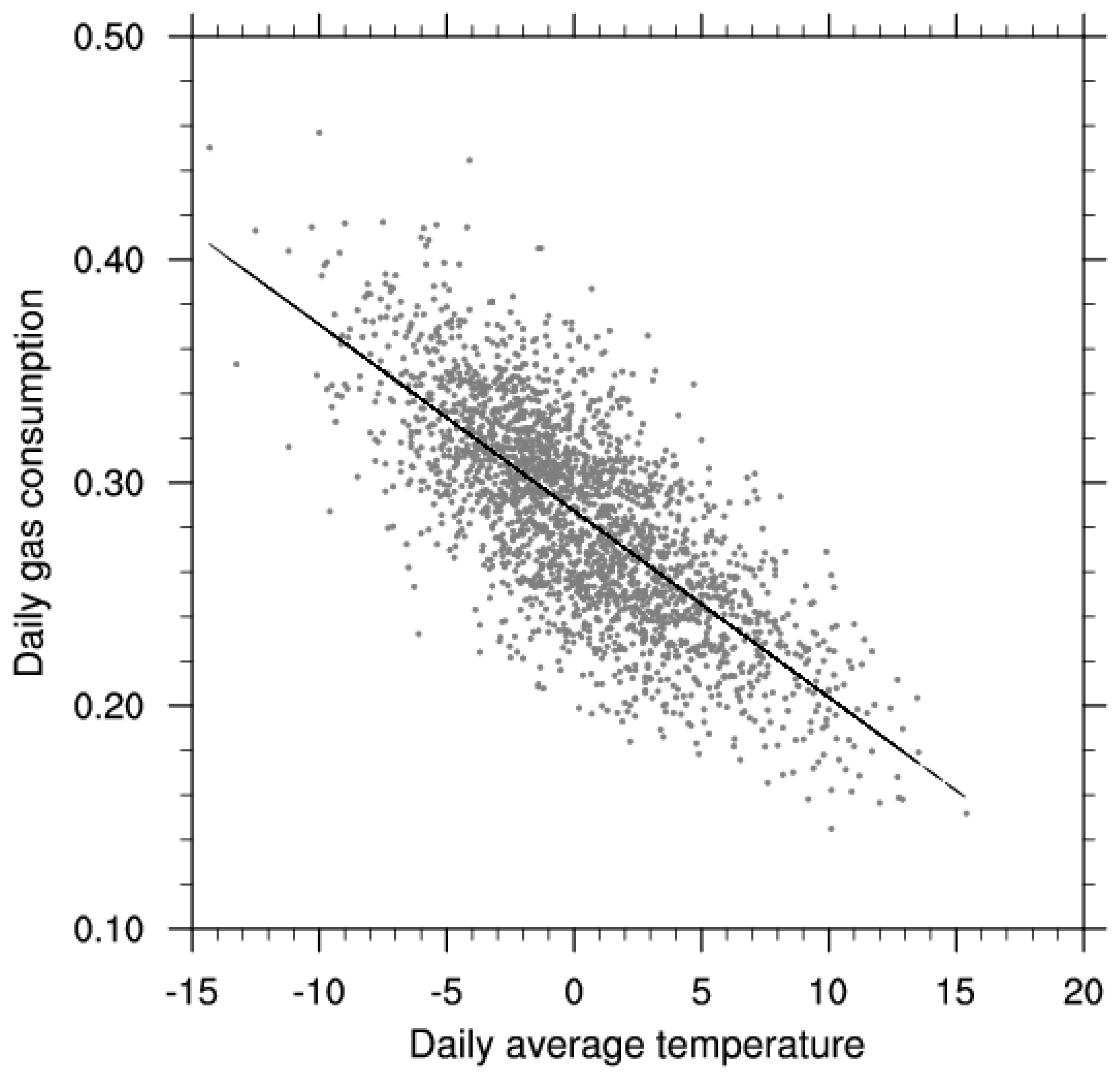
3.1. Response of the Natural Gas Consumption to Temperature

Figure 2 shows the scatterplot of daily natural gas consumption normalized by GDP and daily average temperature during heating season for the period of 2002–2021 in Beijing. It is indicated that the daily natural gas consumption normalized by GDP was linearly correlated with the daily average temperature.
Therefore, a linear regression model was used to estimate the response of daily gas consumption to daily average temperature. According to the least-square method, the regression coefficient α was approximately −0.0040, and the constant c was approximately 0.1316. Therefore, Equation (4) could be rewritten as
G A S t ^ = 0.0040 T t + 0.1316 .
The correlation between the daily natural gas consumption and daily average temperature was as high as 0.79, significant at the 95% confidence level according to a two-tailed Student’s t test. Thus, the temperature explained approximately 62% of the variance of the residual gas consumption normalized by GDP. Moreover, the impact of the COVID-19 pandemic since 2019 was examined by excluding the data for this period, and the results showed that its impact on the normalized natural gas consumption was weak and negligible (figure not shown).

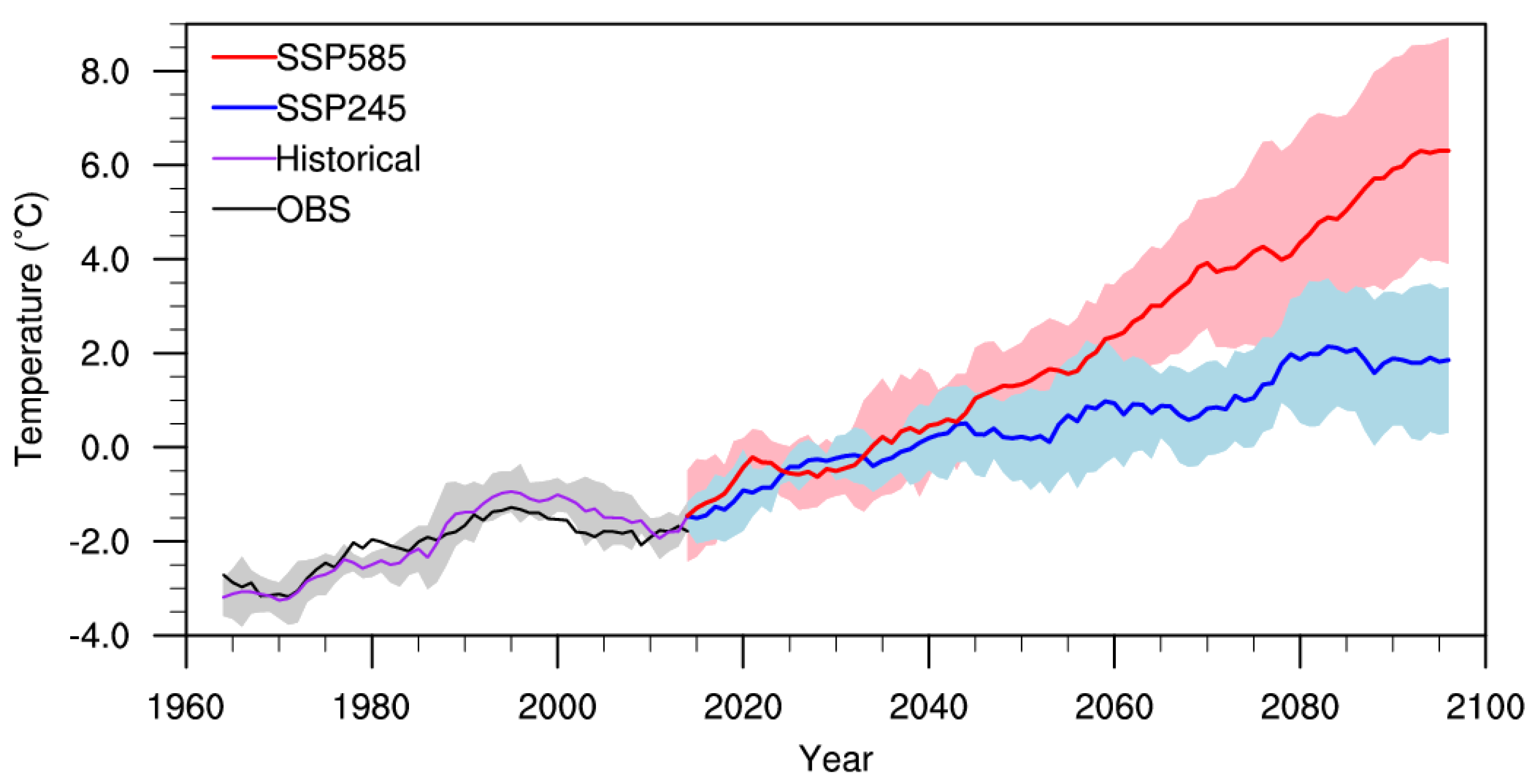
3.2. Changes under Future Scenarios

It is generally assumed that climate models, which have a better performance in reproducing past climate changes, might also be able to simulate future changes with higher accuracy [23,24]. To estimate temperature-related changes in the natural gas consumption under future scenarios, we first examined the performance of 37 CMIP6 models to simulate past changes in the winter mean temperature during 1960–2014 in Beijing (see Figure 3). To eliminate interannual signals and focus on long-term variability, a 9 year running average was applied to the time series of the winter mean temperature. It is indicated in Figure 3 (red line) that the observed winter mean temperature showed a rising trend from the 1970s to the late 1990s before slowing down, which is consistent with the global warming hiatus in the last two decades [25,26,27,28]. However, only a few models simulated a change in the winter mean temperature similar to that of the observed one (see blue lines in Figure 3). In particular, the correlation between the observed and simulated winter mean temperature was higher than 0.75 in CanESM5-CanOE, CNRM-CM6-1-HR, CNRM-CM6-1, FGOALS-f3-L, and NorESM2-MM, with significance above the 95% confidence level according to a two-tailed Student’s t-test, in which the effective number of degrees of freedom was estimated following Davis [29]. Thus, these five models were selected to construct the multi-model ensemble mean of the winter mean temperature for the future projection of the natural gas consumption in Beijing.
Figure 4 displays the multi-model ensemble mean and spread of the winter mean temperature for the historical simulations during 1960–2014, as well as under SSP245 and SSP585 scenario simulations during 2015–2100 in Beijing. It is shown that changes in the multi-model ensemble mean for the historical simulation (purple line) highly resembled those in the observation (black line), with a correlation value of 0.93 during 1960–2014. The winter mean temperature would increase gradually under the SSP245 scenario (blue line) but rapidly under the SSP585 scenario (red line) from the early 2040s to the end of the 21st century, which is consistent with the result explored in previous studies [30]. Relative to the period of 1995–2014 (Table 2), the change in the winter mean temperature would be approximately 1.75 °C (±0.80 °C) for the period of 2041–2050 and 3.28 °C (±1.54 °C) for the period of 2091–2100 under the SSP245 scenario, whereas, under the SSP585 scenario, the change would increase from 2.41 °C (±0.80 °C) for the period of 2041–2050 to 7.66 °C (±2.32 °C) for the period of 2091–2100.
Corresponding to changes in the winter mean temperature, the natural gas consumption would show a decrease trend during 2015–2100 under both the SSP245 and the SSP585 scenarios (Figure 5). Consistent with that in the winter mean temperature, the difference in the natural gas consumption between the SSP245 and SSP585 scenarios would be relatively small before early 2040s but become larger after that. Relative to that for the period of 1995–2014 (Table 2), the natural gas consumption would show a reduction of approximately 5% (±2%) for the period of 2041–2050 and 9% (±4%) for the period of 2091–2100 under the SSP245 scenario. The reduction in the natural gas consumption would be more obvious, reaching 22% (±7%) for the period of 2091–2100, under the SSP585 scenario.

4. Conclusions and Discussion

During the heating season from middle November to the following middle March, the natural gas consumption is primarily dominated by residential heat supply in Beijing, China [7]. After eliminating the influence of socioeconomic factors (such as population trend and economic structure) on heating demand, the daily natural gas consumption had a nearly linear response to the daily average temperature during heating season in the past two decades in Beijing. Hence, a linear regression model was built to estimate temperature-related changes in the natural gas consumption under future warming scenarios. This is somewhat different from previous studies [11,15], which employed a log-linear regression model to estimate the natural gas consumption response to temperature.
To reduce uncertainty in the projection, five out of the 37 CMIP6 models analyzed in this study were selected to construct a multi-model ensemble mean of the temperature for projection. It was shown that these five CMIP6 models, namely, CanESM5-CanOE, CNRM-CM6-1-HR, CNRM-CM6-1, FGOALS-f3-L, and NorESM2-MM, had a better performance in reproducing past changes in the winter mean temperature in Beijing, especially the warming trend from the 1970s to late 1990s, as well as the warming hiatus in the last two decades. The multi-model ensemble mean of the winter mean temperature in Beijing would increase gradually under the SSP245 scenario but rapidly under the SSP585 scenario from the early 2040s to the end of 21st century, leading to an obvious decrease in the natural gas consumption under the high-emission scenario. Relative to that in present day (1995–2014), the natural gas consumption would show a reduction of approximately 9% (±4%) at the end of 21st century (2091–2100) under the SSP245 scenario and approximately 22% (±7%) under the SSP585 scenario, which is consistent with the findings in [11] for the Greater Dublin Region, Ireland and in [15] for California, United States. This implies that the linear regression method used to estimate temperature-related changes in the natural gas consumption and the method used to select climate models for future projection in this study can be applied in other regions. Moreover, the findings obtained in this study can contribute to an understanding of the climate change impact on regional natural gas consumption under future warming scenarios in East Asia.
Previous studies revealed that natural gas consumption tends to increase with population and economic growth [9,16,31]. The present study only detected the effect due to temperature changes in response to anthropogenic greenhouse gas emissions, while the socioeconomic factors were held constant. Reductions in natural gas consumption due to rising temperature may be offset by an increase in the population trend and other socioeconomic factors, which deserves further investigation in future works. Moreover, global warming tends to cause decreased energy demand for heating and increased energy demand for cooling [12,13,15]. However, the relationship between temperature and electricity consumption from space cooling and the difference in the energy demand between heating and cooling in Beijing and adjacent regions remain unclear, which are also issues that need to be addressed in future works.

Author Contributions

Conceptualization, J.M. and Y.D.; Methodology, Software and Validation, J.M. and Y.D.; Formal analysis, Y.D. and H.W.; Writing Original Draft, J.M. and Y.D.; Review and Editing, H.W.; Supervision, J.M.; Funding and Acquisition, J.M. and Y.D. All authors have read and agreed to the published version of the manuscript.

Funding

This research was funded by the National Key Research Program and Development of China (2018YFF0300105).

Institutional Review Board Statement

Not applicable.

Informed Consent Statement

Not applicable.

Data Availability Statement

The fifth generation of atmospheric reanalysis in European Centre for Medium-Range Weather Forecasts (ERA5 reanalysis) are from https://www.ecmwf.int/en/forecasts/datasets/reanalysis-datasets/era5 (accessed on 21 June 2022). The CMIP6 data are available at https://pcmdi.llnl.gov/CMIP6/ (accessed on 21 June 2022). The observed temperature data and natural gas consumption are provided by the Beijing Meteorological Service Center, while the socioeconomic data are obtained from the Beijing Statistical Yearbooks. These data are available from the corresponding author upon reasonable request.

Acknowledgments

The authors give their special thanks to Jinqing Zuo for useful discussions and comments. The authors are grateful to the three anonymous reviewers for their insightful comments, which helped us improve the quality of this paper.

Conflicts of Interest

The authors declare no conflict of interest.

References

  1. Scharf, H.; Arnold, F.; Lencz, D. Future natural gas consumption in the context of decarbonization—A meta-analysis of scenarios modeling the German energy system. Energy Strateg. Rev. 2021, 33, 100591. [Google Scholar] [CrossRef]
  2. Jaramillo, P.; Griffin, W.M.; Matthews, H.S. Comparative life cycle air emissions of coal, domestic natural gas, LNG, and SNG for electricity generation. Environ. Sci. Technol. 2007, 41, 6290–6296. [Google Scholar] [CrossRef] [PubMed]
  3. Agrawal, K.K.; Jain, S.; Jain, A.K.; Dahiya, S. Assessment of greenhouse gas emissions from coal and natural gas thermal power plants using life cycle approach. Int. J. Environ. Sci. Technol. 2014, 11, 1157–1164. [Google Scholar] [CrossRef] [Green Version]
  4. Wang, S.; Su, H.; Chen, C.; Tao, W.; Streets, D.G.; Lu, Z.; Zheng, B.; Carmichael, G.R.; Lelieveld, J.; Pöschl, U.; et al. Natural gas shortages during the “coal-to-gas” transition in China have caused a large redistribution of air pollution in winter 2017. Proc. Natl. Acad. Sci. USA 2020, 117, 31018–31025. [Google Scholar] [CrossRef]
  5. State Council of the People’s Republic of China. The Air Pollution Prevention and Control National Action Plan. 2013. Available online: https://www.gov.cn/zwgk/2013-09/12/content_2486773.htm (accessed on 10 June 2022).
  6. Cai, S.; Wang, Y.; Zhao, B.; Wang, S.; Chang, X.; Hao, J. The impact of the “Air Pollution Prevention and Control Action Plan” on PM2.5 concentrations in Jing–Jin–Ji region during 2012–2020. Sci. Total Environ. 2017, 580, 197–209. [Google Scholar] [CrossRef] [PubMed]
  7. Zhao, B.; Zheng, H.; Wang, S.; Smith, K.R.; Lu, X.; Aunan, K.; Gu, Y.; Wang, Y.; Ding, D.; Xing, J.; et al. Change in household fuels dominates the decrease in PM2.5 exposure and premature mortality in China in 2005–2015. Proc. Natl. Acad. Sci. USA 2018, 115, 12401–12406. [Google Scholar] [CrossRef] [Green Version]
  8. Eyre, N.; Baruah, P. Uncertainties in future energy demand in UK residential heating. Energy Policy 2015, 87, 641–653. [Google Scholar] [CrossRef]
  9. Etokakpan, M.U.; Akadiri, S.S.; Alola, A.A. Natural gas consumption-economic output and environmental sustainability target in China: An N-shaped hypothesis inference. Environ. Sci. Pollut. Res. 2021, 28, 37741–37753. [Google Scholar] [CrossRef]
  10. Intergovernmental Panel on Climate Change (IPCC). Climate Change 2014: Synthesis Report. Contribution of Working Groups I, II and III to the Fifth Assessment Report of the Intergovernmental Panel on Climate Change; IPCC: Geneva, Switzerland, 2014; p. 151. [Google Scholar]
  11. Liu, X.; Sweeney, J. The impacts of climate change on domestic natural gas consumption in the Greater Dublin Region. Int. J. Clim. Change Strateg. Manag. 2012, 4, 161–178. [Google Scholar] [CrossRef]
  12. Auffhammer, M.; Baylis, P.; Hausman, C.H. Climate change is projected to have severe impacts on the frequency and intensity of peak electricity demand across the United States. Proc. Natl. Acad. Sci. USA 2017, 114, 1886–1891. [Google Scholar] [CrossRef] [Green Version]
  13. Wenz, L.; Levermanna, A.; Auffhammere, M. North–south polarization of European electricity consumption under future warming. Proc. Natl. Acad. Sci. USA 2017, 114, E7910–E7918. [Google Scholar] [CrossRef] [Green Version]
  14. Berardi, U.; Jafarpur, P. Assessing the impact of climate change on building heating and cooling energy demand in Canada. Renew. Sustain. Energy Rev. 2020, 121, 109681. [Google Scholar] [CrossRef]
  15. Auffhammer, M. Climate Adaptive Response Estimation: Short and long run impacts of climate change on residential electricity and natural gas consumption. J. Environ. Econ. Manag. 2022, 114, 102669. [Google Scholar] [CrossRef]
  16. Min, J.; Wang, H.; Dong, Y. Forecast of natural gas consumption in heating season based on EMD and BP neural network methods in Beijing. J. Arid. Meteorol. 2021, 39, 864–870. (In Chinese) [Google Scholar] [CrossRef]
  17. Reyna, J.; Chester, M. Energy efficiency to reduce residential electricity and natural gas use under climate change. Nat. Commun. 2017, 8, 14916. [Google Scholar] [CrossRef] [PubMed]
  18. O’Neill, B.C.; Kriegler, E.; Ebi, K.L.; Kemp-Benedict, E.; Riahi, K.; Rothman, D.S.; van Ruijven, B.J.; van Vuuren, D.P.; Birkmann, J.; Kok, K.; et al. The roads ahead: Narratives for shared socioeconomic pathways describing world futures in the 21st century. Glob. Environ. Change 2017, 42, 169–180. [Google Scholar] [CrossRef] [Green Version]
  19. Eyring, V.; Bony, S.; Meehl, G.A.; Senior, C.A.; Stevens, B.; Stouffer, R.J.; Taylor, K.E. Overview of the Coupled Model Intercomparison Project Phase 6 (CMIP6) experimental design and organization. Geosci. Model Dev. 2016, 9, 1937–1958. [Google Scholar] [CrossRef] [Green Version]
  20. Hempel, S.; Frieler, K.; Warszawski, L.; Schewe, J.; Piontek, F. A trend-preserving bias correction–the ISI-MIP approach. Earth Syst. Dyn. 2013, 4, 219–236. [Google Scholar] [CrossRef] [Green Version]
  21. Carleton, T.A.; Hsiang, S.M. Social and economic impacts of climate. Science 2016, 353, aad9837. [Google Scholar] [CrossRef] [Green Version]
  22. Schlenker, W.; Roberts, M.J. Nonlinear temperature effects indicate severe damages to U.S. crop yields under climate change. Proc. Natl. Acad. Sci. USA 2009, 106, 15594–15598. [Google Scholar] [CrossRef] [Green Version]
  23. Stoner, A.M.K.; Hayhoe, K.; Wuebbles, D.J. Assessing General Circulation Model Simulations of Atmospheric Teleconnection Patterns. J. Clim. 2009, 22, 4348–4372. [Google Scholar] [CrossRef]
  24. Wu, M.; Zhou, T.; Li, C.; Li, H.; Chen, X.; Wu, B.; Zhang, W.; Zhang, L. A very likely weakening of Pacific Walker Circulation in constrained near-future projections. Nat. Commun. 2021, 12, 6502. [Google Scholar] [CrossRef] [PubMed]
  25. Easterling, D.R.; Wehner, M.F. Is the climate warming or cooling? Geophys. Res. Lett. 2009, 36, L08706. [Google Scholar] [CrossRef] [Green Version]
  26. Foster, G.; Rahmstorf, S. Global temperature evolution 1979–2010. Environ. Res. Lett. 2011, 6, 044022. [Google Scholar] [CrossRef]
  27. Fyfe, J.; Gillett, N.; Zwiers, F. Overestimated global warming over the past 20 years. Nat. Clim. Change 2013, 3, 767–769. [Google Scholar] [CrossRef]
  28. Li, X.; Wu, Z.; Li, Y. A link of China warming hiatus with the winter sea ice loss in Barents–Kara Seas. Clim. Dyn. 2019, 53, 2625–2642. [Google Scholar] [CrossRef]
  29. Davis, R.E. Predictability of sea surface temperature and sea level pressure anomalies over the North Pacific Ocean. J. Phys. Oceanogr. 1976, 6, 249–266. [Google Scholar] [CrossRef]
  30. Wu, J.; Gao, X. Present day bias and future change signal of temperature over China in a series of multi-GCM driven RCM simulations. Clim. Dyn. 2020, 54, 1113–1130. [Google Scholar] [CrossRef] [Green Version]
  31. Zhu, R.; Qiao, J.; Wang, X.; Jiang, X. Statistical analysis of main factors of natural gas consumption growth in Beijing city. Gas Heat 2017, 37, 26–30. [Google Scholar]
Figure 1. Time series of the daily average natural gas consumption (unit: m3) during heating season for the period of 2002–2021 in Beijing.
Atmosphere 13 01178 g001
Figure 2. Scatterplot of the daily natural gas consumption normalized by GDP and daily average temperature (unit: °C) during heating season for the period of 2002–2021 in Beijing. The solid line denotes the linear fitting of the dots.
Atmosphere 13 01178 g002
Figure 3. Nine year smoothed time series of the winter mean temperature (unit: °C) derived from the historical simulations (blue line) for the individual models during 1960–2014 in Beijing. The x-axis refers to the year, while the y-axis refers to the temperature. The red line denotes the observation, and R is the correlation between the observation and simulation.
Atmosphere 13 01178 g003
Figure 4. Multi-model ensemble means of the 9 year smoothed winter mean temperature (unit: °C) for the historical simulations (purple line) during 1960–2014, as well as the simulations under the SSP245 (blue line) and SSP585 (red line) scenarios during 2015–2100 in Beijing. The black line denotes the observation, and shadings indicate the model spread.
Atmosphere 13 01178 g004
Figure 5. Percentage changes in the 9 year smoothed natural gas consumption with respect to temperature changes under the SSP245 (blue line) and SSP585 (red line) scenarios during heating season for the period of 2015–2100 (relative to 1995–2014) in Beijing. Shadings denote the model spread.
Atmosphere 13 01178 g005
Table 1. Name, institute, and horizontal resolution of the CMIP6 models used in the present study. R denotes correlation between the observed and simulated winter-mean temperature during 1960–2014 in Beijing; * significance at the 95% confidence level according to a two-tailed Student’s t-test.
ModelInstituteResolution
(Lon × Lat)
R
ACCESS-CM2Commonwealth Scientific and Industrial Research Organisation (CSIRO) and Australian Research Council Centre of Excellence for Climate System Science, Australia192 × 1440.16
ACCESS-ESM1-5CSIRO, Australia192 × 1450.56
AWI-CM-1-1-MRAlfred Wegener Institute, Helmholtz Center for Polar and Marine Research, Germany384 × 1920.24
BCC-CSM2-MRBeijing Climate Center, China Meteorological Administration, China320 × 1600.18
CAMS-CSM1-0Chinese Academy of Meteorological Sciences, China Meteorological Administration, China320 × 1600.36
CanESM5Canadian Centre for Climate Modeling and Analysis, Canada128 × 640.19
CanESM5-CanOECanadian Centre for Climate Modeling and Analysis, Canada128 × 640.79 *
CESM2National Center for Atmospheric Research, Climate and Global Dynamics Laboratory, USA288 × 1920.55
CESM2-WACCMNational Center for Atmospheric Research, Climate and Global Dynamics Laboratory, USA288 × 192−0.20
CNRM-CM6-1-HRCNRM and Centre Europeen de Recherches et de Formation Avancee en Calcul Scientifique (CERFACS), FranceT3590.91 *
CNRM-CM6-1CNRM–CERFACS, FranceT1270.76 *
CNRM-ESM2-1CNRM–CERFACS, FranceT1270.00
EC-Earth3EC—Earth consortium512 × 2560.63
EC-Earth3-CCEC—Earth consortium512 × 2560.01
EC-Earth3-VegEC—Earth consortium512 × 256−0.28
EC-Earth3-Veg-LREC—Earth consortium320 × 1600.55
FGOALS-g3Institute of Atmospheric Physics (IAP), Chinese Academy of Sciences, China180 × 800.02
FGOALS-f3-LIAP, Chinese Academy of Sciences, China360 × 1800.91 *
GFDL-ESM4National Oceanic and Atmospheric Administration, USA360 × 180−0.77
GFDL-CM4National Oceanic and Atmospheric Administration, USA360 × 180−0.35
GISS-E2-2-GGoddard Institute for Space Studies, USA144 × 900.22
GISS-E2-1-HGoddard Institute for Space Studies, USA144 × 900.56 *
GISS-E2-1-GGoddard Institute for Space Studies, USA144 × 90−0.01
HadGEM3-GC31-LLMet Office Hadley Centre, UK192 × 1440.00
HadGEM3-GC31-MMMet Office Hadley Centre, UK432 × 324−0.17
INM-CM4-8Institute of Numerical Mathematics, Russia180 × 120−0.58
INM-CM5-0Institute of Numerical Mathematics, Russia180 × 120−0.41
IPSL-CM6A-LRInstitut Pierre Simon Laplace, France144 × 1430.27
KACE-1-0-GNational Institute of Meteorological Sciences, Korea192 × 1440.38
MIROC6Atmosphere and Ocean Research Institute, University of Tokyo, Japan256 × 1280.32
MIROC-ES2LAtmosphere and Ocean Research Institute, University of Tokyo, Japan128 × 640.39
MPI-ESM1-2-HRMax Planck Institute for Meteorology, Germany384 × 192−0.22
MPI-ESM1-2-LRMax Planck Institute for Meteorology, Germany192 × 960.31
MRI-ESM2-0Meteorological Research Institute, Japan320 × 1600.46
NorESM2-LMNorwegian Climate Center, Norway144 × 960.53 *
NorESM2-MMNorwegian Climate Center, Norway288 × 1920.77 *
UKESM1-0-LLMet Office Hadley Centre, UK192 × 1440.09
Table 2. Percentage changes in the natural gas consumption (unit: %) with respect to temperature changes (unit: °C) during heating season under the SSP245 and SSP585 scenarios relative to 1995–2014 in Beijing. Values in the bracket denote the model spread.
YearsSSP245SSP585
ΔTempΔGasΔTempΔGas
2021–20300.92 (0.27)−2.83 (1.12)0.98 (0.59)−2.16 (1.68)
2031–20401.31 (0.45)−3.26 (1.33)1.52 (1.04)−4.33 (3.17)
2041–20501.75 (0.80)−4.68 (2.41)2.41 (0.80)−7.02 (3.08)
2051–20602.02 (1.16)−5.80 (3.64)3.24 (1.06)−8.78 (3.04)
2061–20702.21 (0.93)−6.69 (2.26)4.61 (1.26)−12.75 (3.32)
2071–20802.75 (0.96)−7.00 (2.95)5.47 (2.02)−15.79 (5.82)
2081–20903.38 (1.41)−9.68 (3.56)6.66 (2.20)−18.31 (5.93)
2091–21003.28 (1.54)−9.15 (4.19)7.66 (2.32)−21.55 (6.76)
Publisher’s Note: MDPI stays neutral with regard to jurisdictional claims in published maps and institutional affiliations.

