Article

Predicting Indian Ocean Cyclone Parameters Using an Artificial Intelligence Technique

1
Andhra Pradesh State Disaster Management Authority, Kunchanapalli 522501, Andhra Pradesh, India
2
Center for Ocean-Atmospheric Prediction Studies, The Florida State University, Tallahassee, FL 32310, USA
*
Author to whom correspondence should be addressed.
Atmosphere 2022, 13(7), 1157; https://doi.org/10.3390/atmos13071157
Submission received: 17 June 2022 / Revised: 18 July 2022 / Accepted: 19 July 2022 / Published: 21 July 2022
(This article belongs to the Section Atmospheric Techniques, Instruments, and Modeling)

Abstract

:
Precise prediction of a cyclone track with wind speed, pressure, landfall point, and the time of crossing the land are essential for disaster management and mitigation, including evacuation processes. In this paper, we use an artificial neural network (ANN) approach to estimate the cyclone parameters. For this purpose, these parameters are obtained from the International Best Track Archive for Climate Stewardship (IBTrACS), from the National Oceanic and Atmospheric Administration (NOAA). Since ANN benefits from a large number of data points, each cyclone track is divided into different segments. We use past information to predict the geophysical parameters of a cyclone. The predicted values are compared with the observations.

1. Introduction

A tropical cyclone (TC) is one of the deadliest and most damaging natural disasters affecting people, livestock, agriculture, and the economics of coastal areas. Reductions in uncertainty are of great benefit for disaster-management authorities to plan for evacuation and mitigation processes [1,2]. The major components of cyclone warnings are forecasts of the track, winds, and pressure, in addition to a precise landfall point with the time of crossing the land. Predicting the track of a cyclone helps in knowing the direction in which it is moving and the area it is likely to affect. The intensity is primarily estimated from the maximum sustained wind speed, which provides a measure for the severity of a cyclone. The wind is one of the major hazards associated with a TC, as it creates damage to houses, bridges, electrical poles, mangroves, and the ecosystem. While the damage in the coastal region is typically quite high, inland damage cannot be ruled out. Strong winds are present at the eyewall of a cyclone. The intensity of a cyclone together with the wind speed and the pressure aids in predicting the storm surge, although the spatial extent of the storm and the direction of travel are also important in the prediction process [3,4]. A storm surge is the most devastating component of cyclones, particularly along coastlines that have a highly varying bathymetry, which are plentiful in India. Since bathymetry is one of the most critical components in estimating a storm surge, even a slight error in predicting the landfall point can lead to different storm-surge heights. The time of crossing the land is used to include the impacts of tides and to help in arranging the evacuation process. Thus, location, winds, and the pressure of a cyclone, as well as the landfall point and the time of land crossing, are the critical components in predicting the storm surge.
Several dynamiccal, statistical, and statistical–dynamic models have been developed to predict cyclone parameters. Mohanty and Gupta [5] and Gupta [6] summarised different track-prediction techniques. Bell [7] described the operational forecasting models. Ali et al. [8] summarised the different approaches used in predicting cyclones. They used the Artificial Neural Network (ANN) technique to predict the position of a cyclone alone, in terms of the latitude and longitude using the previous 12 h of observations. In this paper, we attempt to use the same technique to predict winds, pressure, and landfall, in addition to the storm location in terms of latitude and longitude.
ANN is a powerful data-mining tool for computing input–output relationships. It is an information-processing paradigm that works somewhat like a hypothesized biological system in the human brain. ANN consists of an interconnected assembly of models, with functionality that is based on a neuron [9]. The analysis can be used as a standalone application or as a complement to statistical analysis. This non-dynamic numerical model has been used in many oceanographic [10,11,12,13,14,15] (and meteorological studies [16,17,18]. The ANN technique is also useful for satellite-parameter retrievals [19,20,21,22]. Multiple linear regression (MLR) is a method dealing with linear dependencies, whereas neural networks deal with nonlinearities. If data has some nonlinear dependencies, neural networks outperform the MLR approach. In addition, many studies have used statistical and machine-learning techniques for cyclone studies because those techniques require less computing time. For example, Swain et al. [9] concluded that the ANN approach gave a better result compared to multiple linear-regression techniques (MLR) in the estimation of mixed-layer depth. Sharma et al. [21] also demonstrated the benefits of the ANN technique over MLR. Hence, we used the ANN approach in this study. ANN requires three sets of data: one for training, another for verification, and a third for validation. The first dataset is used to train the model, the second dataset is used to test the model for any shortcomings, and finally, the validation dataset is used in statistical-parameter estimation. The validation dataset is independent: it is not considered in developing the model. In an ANN model, both the input and output variables are normalized to vary between 0 and 1. Popular ANN models include radial-basis functions (RBF) and multilayer perceptions (MLP).

2. Date and Methodology

2.1. Data

Cyclone parameters available over the north Indian Ocean from IBTrACS (International Best Track Archive for Climate Stewardship, https://www.ncei.noaa.gov/data/international-best-track-archive-for-climate-stewardship-ibtracs/v04r00/access/csv/) (accessed on 29 January 2021) during 1971–2019 are used in this analysis. IBTrACS provides information on cyclones from different sources. Here, we use JTWC (Joint Typhoon Warning Center) data alone. These data contain latitude, longitude, surface central pressure, and maximum wind speed of cyclones. Although these data are available both at 3- and 6-h intervals, we use only 6-h interval data in this study because the number of cases with 3-h intervals is much smaller. Based on availability, also used in this study are wind field data from 1973 to 2019, pressure field data from 2001 to 2019, and position (latitude and longitude) data from 1971 to 2019. It is better to have a large number of observations for ANN analysis. If we consider only the period for which pressure fields are available, the dataset would become smaller, so the errors would be larger. Hence, we consider the periods as they are available. However, a segmentation procedure (described later) is used to increase the number of points for ANN analysis. After eliminating those cyclone positions at irregular intervals, 323 cyclones are studied for position, 239 cyclones for wind speed, and 104 cyclones for pressure. An ANN approach is used to forecast future position using past cyclone observations. The tracks are segmented to provide the number of records required by ANN. The selection of training, verification, and validation is described in the next section.

2.2. Segmentation of the Tracks

ANN requires a large number of data records (i.e., sets of conditions for a specific time) to develop the model. Since we do not have enough points if we consider the actual cyclone points rather than just landfall points, each cyclone track has been divided into different segments. A schematic representation of the procedure adopted for segmentation into a 24-h forecast with 6-h interval data is given in Figure 1. For example, for a 24-h forecast if the present position (in terms of latitude and longitude) is at point 3 in Figure 1, that position as well as the previous two six-hour positions (at 2 and 1) are considered as the predictors, and the position at 7 after 24 h from the present position is taken as the predictand. Thus, the positions for the predictors for this first segment are 1, 2, and 3, and the predictand is 7 (pink line). For example, if the present position is at 18 h, locations of 6, 12, and 18 h are the predictors (current and past positions), and the location at 18 h (the next day) is the predictand (forecast position). Then, the second segment is moved to position 2 after 6 h and, for the second segment, positions at 2, 3, and 4 are the predictors, and position at 8 is the predictand (magenta line). Similarly, for segment 12, positions at 10, 11, and 12 are the predictors, and position at 16 is the predictand.
Since ANN requires three sets of data (one for training, another for verification, and a third for validation), out of the total of 49 years of data on latitude and longitude from 1971 to 2019, 20 years from 1971 to 1990 are used for training, 17 years from 1991 to 2007 for verification, and 12 years from 2008 to 2019 for validation. The same analysis is repeated for cyclone wind speed and pressure. Since these three parameters have different periods, the periods used for training, verification, and validation are also different, as reported in Table 1. In this analysis, the Multi-Layer Perceptron (MLP) approach is used. The period of study, the number of past hours used as predictors, and the hour of forecast as predictand, as well as the total number of segments used for training, verification, and validation for cyclone position, wind speed, and pressure, are given in Table 1. The first column in the table indicates the past number of hours used as the predictors, and the second column indicates the hours in advance for which the forecast is given as the predictand. Thus, a forecasted time of 6 h using the past 6 h has the two past six hourly positions in addition to the current position as predictors and the future 6 positions as predictands. As explained earlier, the total number of points in each dataset depends on the type of segmentation and the period of the data availability. Thus, the number of records decreases as the forecasted time increases from 6 h to 24 h, besides the past number of hours used as predictors.
The land-crossing position of the cyclone track at the coastline has been computed using ArcGIS software.

3. Results and Discussion

The cyclone position in terms of latitude and longitude, pressure, and wind speed are estimated from an ANN approach and compared with the observations in the following sections.

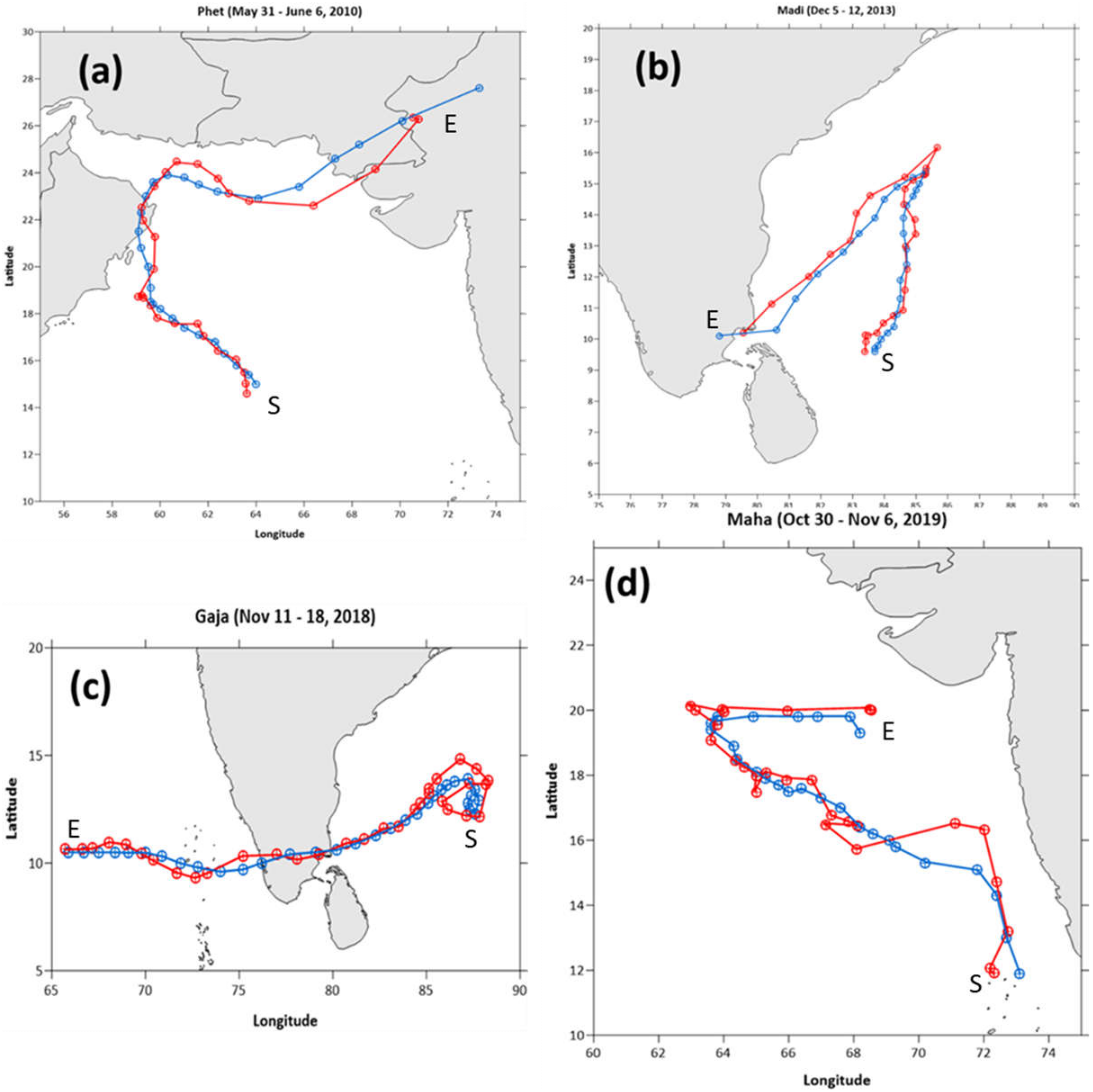
3.1. Comparison of the Position

Forecast of the cyclone position in terms of the latitude and longitude are predicted for 6, 12, 18, and 24 h in advance using the current position and 6- and 12-h past positions. The skill in prediction dropped if the forecast period is increased beyond 24 h. Thus, there are two forecasts (latitude and longitude) for 6, 12, 18, and 24 h using 6- and 12-h past positions. Thus, altogether there are eight forecasts. The forecast statistics are given separately for the latitude and longitude in Table 2. Statistics for longitude are indicated in parenthesis. The Pearson Correlation Coefficient (CC) for all forecasts for each of the three datasets (training, testing, and validation) is greater than 0.97, which shows that the patterns of change in the estimations are well-captured. Comparable values among the three datasets for all statistical parameters indicate that they share similar characteristics. Further, the Absolute Residual Mean (ARM) and Root Mean Square Error (RMSE) for longitude are greater than those for latitude in all three dataset forecasts. This is because the longitude values (ranging from 50 to 100 degrees) are greater than the latitude values (ranging from 0 to 25 degrees), because the correlation does not indicate goodness of fit but indicates goodness of patterns of change (i.e., the change in the predicted variable is proportional to the change in the comparison data). That proportionality could be way off and not impact the correlation. Hence, emergency managers will probably find the RMSE value more useful than the correlation.
The Mean Distance Error (MDE) between the observed and predicted positions are computed using 6- and 12-h past positions for the lead hours of 6, 12, 18, and 24. Thus, altogether eight forecasts are given, as shown in Figure 2. This error, for all the cyclones together, varies from 30.7 km (06P06F) to 151.7 km (12P24F). For example, the mean distance error for the 6-h past positions (as input) and 24-h lead position (as the output) is 139.14 km (06P24F in Figure 2). Ali et al. [8] reported an MDE of 137.5 km using ANN and 182.5 km using the CLIPER approach [23,24] for the same 6-h past positions (as input) and 24-h lead position (as the output). Hence, we do not repeat the comparison of the track errors from the ANN approach and CLIPER in this paper. The MDE between the best track and predicted tracks are almost the same for 6-h ANN forecasts, based on a 6-h lead time and a 12-h lead time.
The error increases from 6-h forecast (30.68 Km) to 24-h forecast (139.14 km) for 6-h interval data by considering the 6-h past positions. Similarly, the error increases from 6-h forecast (32.99 km) to 24-h forecast (151.68 km) by considering the 12-h past positions. From the validation dataset, four cyclones that do not have a straight path (Phet, Madi, Gaja, and Maha) are randomly selected. A comparison of the best track and the predicted track for these four cyclones is shown in Figure 3. First, the very severe cyclonic storm, Phet (31 May to 6 June 2010) (Figure 3a), initially moved northwestward, then curved after passing over the land, and moved northeastward. The ANN’s predicted track very nearly followed this best track, with an MDE of 82.5 km. Another very severe cyclonic storm, Madi (5–12 December 2013) (Figure 3b), re-tracked after moving northeastward, and the predicted track is similar to the best track, with an MDE of 53.1 km. This is the least among the four cyclones studied. Gaja, another severe cyclonic storm (11–18 November 2018), began its track by looping almost back to its starting position in the Bay of Bengal, then it crossed the Indian landmass and moved over the Arabian Sea, with an MDE of 75 km. In addition, finally, the extremely severe cyclonic storm, Maha (30 October to 6 November 2019), has the largest MDE of 87.8 km. The errors are large in the beginning but reduce as the storm progresses. The only reason we could find for the sudden changes in direction of the Maha cyclone is that its speed varied significantly during its course. The minimum and maximum distances it traveled in 6 h are 9.97 km and 244.55 km, respectively. Atlantic Ocean storms that change in speed are typically associated with storms undergoing extratropical transition, but that is not normally a consideration for Indian Ocean storms. Other than this extreme (and, hence, hard to train for) change in speed, we could not find any other reason for the large deviations of the predicted track from the best track of the Maha cyclone. We also plotted (figures not shown) the predicted and best tracks for which the MDE is the minimum (33.45 km) and maximum (120.2 km). The difference between the predicted and the best track for the maximum MDE is much less than that for the Maha cyclone.

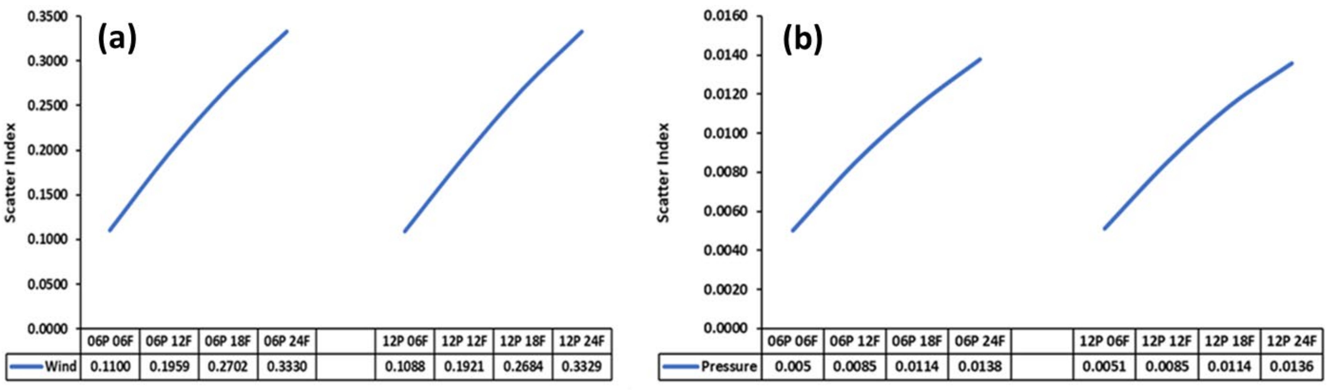
3.2. Estimation of Wind Speed

Statistical parameters such as ARM, RMSE, SI (Scatter Index), and CC for all eight forecast combinations for training, verification, and validation are given in Table 2. The CC is more than 0.78 for all estimations of the validation dataset. The RMSE varies between 5 and 16 knots depending upon the lead time. The SI, which is one of the best statistical parameters to interpret any estimation, varies between ~0.1 for a 6-h advance prediction to ~0.3 for a 24-h advance prediction for the validation dataset (Table 2 and Figure 4a). The values increase with the lead time, and this increase is the same irrespective of the past number of 6 or 12 h.

3.3. Estimation of Pressure

Estimation of pressure fields of tropical cyclones is a major problem. The statistical parameters in the estimation of pressure for all eight forecast combinations are given in Table 2. The RMSE for the validation dataset varies from 4.9 hPa to 13.7 hPa, with the error increasing with the lead time. The errors are large, as the absolute values themselves are large (on the order of 1000 hPa). Purnachand et al. [25], utilizing the University of Washington Planetary Boundary Layer (UWPBL) model of Patoux et al. [26], estimated the pressure in cyclone Nilam using Ocean Sat-II Scatterometer wind fields. This model has an option providing the background-pressure values. The RMSE from this model is 4.97 hPa if a standard pressure of 1013 hPa was given, however, the error was reduced to 0.67 hPa when the pressure values of all available buoys were utilized. The estimations by Purnachand et al. [25] are a better comparative to ours because they used in situ pressure values as initial conditions. However, our estimations are comparable with theirs, when using a standard pressure value of 1013 hPa.
The SI is very small for all of the eight datasets, varying between 0.0050 and 0.0138 for the validation dataset. The SIs using the 6-h past position and the 12-h past position are shown in Figure 4b. The values increase with the forecast lead time, and this increase is the same irrespective of the past number of 6 or 12 h. In addition to computing the SI, we estimated the skill score (SS) following Murphy [27] (Equation. 3), where the MLR results were considered as the reference. The SS here is 3.9%.

3.4. Land-Crossing-Point Difference

The difference between the land-crossing points indicated by the JTWC’s best tracks and the ANN’s predicted tracks are given in Table 3, for the 12-h past positions as the predictors and the 12-h and 24-h forecasts’ positions as the predictants. For 12-h predictions, the minimum error is 3.8 km, and the maximum error is 124.8 km with a mean value of 38.2 km. In addition, for 24-h forecasts, the minimum error is 0.26 km, and the maximum error is 192.56 km with a mean value of 71.2 km. Mohapatra et al. [28] evaluated the official landfall forecasts by the India Meteorological Department during 2003–2013 for different forecast times ranging from 12 to 72 h. Their average landfall-point-forecast errors are 69 km and 104 km for 12- and 24-h forecasts. During our analysis period of 1971–2019, the average errors are 38 km and 71 km for 12-h and 24-h forecasts, respectively, which are significantly less than those reported by Mohapatra et al. [28].

4. Summary and Conclusions

In this study, an ANN approach is used to predict the cyclone parameters, specifically the position in terms of latitude and longitude, wind speed, and pressure. ANN or other machine approaches are less computationally intense than operational numerical weather-predication models. The predicted track is used to estimate the landfall point. After a quality check, 323 cyclones are used for position, 239 cyclones for wind speed, and 104 cyclones for pressure. Since ANN requires a large amount of data, each cyclone has been divided into segments to increase the number of points. Altogether, eight forecast combinations are studied with input from the past 6 and 12 h, each of these past hours having predictions for 6, 12, 18, and 24 h.
The RMSE (which is more relevant to emergency managers) is greater for longitude than for latitude. The MDE increases with the lead time in both 6- and 12-h past positions. A comparison of the best track from JTWC and the ANN’s predicted track for the four cyclones randomly selected from the validation dataset match satisfactorily, as described below. The four cyclones selected have different tracks such as looped, curved, and re-tracked. The MDE of these four cyclones varies between 53.1 km and 87.8 km.
The SI of wind speed for the validation dataset varies between 0.11 and 0.33, with a CC of more than 0.7 being quite acceptable. As with the position predictions, the SI for the wind speed increases with lead time. Further, whether using the past 6 h or 12 h, the errors remain close to the same.
The SI for the pressure estimation of the validation dataset is negligible, varying from 0.005 to 0.01, with a correlation of more than 0.7. The high values of RMSE are understandable because the pressure values are in the range of 1000 hPa. As in the case of the previous two parameters, the SI increases with lead time and remains similar for the past 6- and past 12-h predictions.
The difference between the JTWC’s best track and ANN’s predictions for landfall-crossing points has a mean error of 38.4 km for the 12-h forecast and 71.02 km for the 24-h forecast; both are significantly less than the official Indian weather-forecast errors. We compared the ANN forecasts with seven dynamical model outputs for 21 cyclones during 2017–2019. Our findings show that an ANN approach outperformed all the numerical models. However, during 2019, ANN results were better than three models but worse than four models. Incidentally, cyclone Maha, with the largest track error, occurred during 2019. By analyzing the 33 cyclones in the north Indian Ocean during 2003–2013, Mohapatra et al. [28] obtained an average error of 69 km for 12-h forecasts and 104 km for 24-h forecasts. Compared to these errors, the errors obtained by the ANN’s predictions are far better. However, Mohapatra et al. [28] were able to predict 72 h in advance, which could not be done in this paper. Since advance notice is critical, the error of 71.02 km needs to be considered.
In the future, we plan to consider either a multiple numerical-model output or output from the same model with different initial conditions to develop an ANN technique for predicting a cyclone’s track.

Author Contributions

Concenptualisation and methodology, M.M.A.; Validation, C.P.C.; Formal analysis, B.H., C.P.C. and M.M.A.; Investigation, M.M.A., M.A.B. and C.P.C.; Data curation, C.P.C. and B.H.; Writing original draft, M.M.A. and C.P.C.; Review and editing, M.A.B. and Y.Z. All authors have read and agreed to the published version of the manuscript.

Funding

This research was funded at Florida State University in part by NASA Physical Oceanography via the Jet Propulsion Laboratory (Contract #1419699) and in part by the Global Ocean Monitoring and Observing Program (Fund #100007298), National Oceanic and Atmospheric Administration, U.S. Department of Commerce, through the Northern Gulf of Mexico Institute (NGI grant number 20-NGI3-106), and partially funded by NASA physical oceanography through the Jet Propulsion Laboratory (Contract #1419699).

Institutional Review Board Statement

Not applicable.

Informed Consent Statement

Not applicable.

Data Availability Statement

All the data used in this study is obtained from the International Best Track Archive for Climate Stewardship (https://www.ncep.noaa.gov/data/international-best-trackarchive-for-climate-stewardship-ibtracs/v04r00/access/csv/, accessed on 29 January 2021).

Acknowledgments

Critical and constructive comments by the anonymous referees improved the quality of the paper. The authors thank their respective departments for their support. Tracy Ippolite helped in editing the manuscript. Cyclone parameters data used from IBTrACS (International Best Track Archive for Climate Stewardship). MAB's contribution was funded in part by NASA Physical Oceanography via the Jet Propulsion Laboratory (Contract #1419699) and in part by the Global Ocean Monitoring and Observing Program (Fund #100007298), National Oceanic and Atmospheric Administration, U.S. Department of Commerce, through the Northern Gulf of Mexico Institute (NGI grant number 20-NGI3-106), and partially funded by NASA physical oceanography through the Jet Propulsion Laboratory (Contract #1419699).

Conflicts of Interest

The authors declare no conflict of interest.

References

  1. Willoughby, H.E.; Rappaport, E.N.; Marks, F.D. Hurricane forecasting: The state of the art. Nat. Hazards Rev. 2007, 8, 45–49. [Google Scholar] [CrossRef] [Green Version]
  2. Lazo, J.K.; Waldman, D.M.; Morrow, B.H.; Thacher, J.A. Household evacuation decision making and the benefits of improved hurricane forecasting: Developing a framework for assessment. Weather Forecast. 2010, 25, 207–219. [Google Scholar] [CrossRef] [Green Version]
  3. Shaji, C.; Kar, S.K.; Vishal, T. Storm surge studies in the North Indian Ocean: A review. Indian J. Geo-Mar. Sci. 2014, 43, 125–147. [Google Scholar]
  4. Rao, A.D.; Poulose, J.; Puja, U.; Mohanty, S. Local-Scale Assessment of Tropical Cyclone Induced Storm Surge Inundation over the Coastal Zones of India in Probabilistic Climate Risk Scenar; Ravela, S., Sandu, A., Eds.; Springer International Publishing: Cham, Switzerland, 2015; pp. 79–88. [Google Scholar] [CrossRef]
  5. Mohanty, U.C.; Gupta, A. Deterministic methods for prediction of tropical cyclone tracks. Mausam 1997, 48, 257–272. [Google Scholar] [CrossRef]
  6. Gupta, A. Current status of tropical cyclone track prediction techniques and forecast errors. Mausam 2006, 57, 151–158. [Google Scholar] [CrossRef]
  7. Bell, G.J. Operational forecasting of tropical cyclones. Aust. Meteorol. Mag. 1979, 27, 249–258. [Google Scholar]
  8. Ali, M.M.; Kishtawal, C.M. Sarika Jain Predicting cyclone tracks in the north Indian Ocean: An artificial neural network approach. Geophys. Res. Lett. 2007, 34, L04603. [Google Scholar] [CrossRef]
  9. Swain, D.; Ali, M.M. Weller Robert. Estimation of mixed-layer depth from surface parameters. J. Mar. Res. 2006, 64, 745–758. [Google Scholar] [CrossRef] [Green Version]
  10. Ali, M.M.; Swain, D.; Weller, R.A. Estimation of ocean subsurface thermal structure from surface parameters: A neural network approach. Geophys. Res. Lett. 2004, 31, L20308. [Google Scholar] [CrossRef] [Green Version]
  11. Tolman, H.; Krasnopolsky, V.; Chalikov, D. Neural network approximations for nonlinear interactions in wind wave spectra: Direct mapping for wind seas in deep water. Ocean Model. 2005, 8, 253–278. [Google Scholar] [CrossRef]
  12. Jain, S.; Ali, M.M. Estimation of sound speed profiles using artificial neural network. IEEE Trans. Geosci. Remote Sens. Lett. 2006, 3, 467–470. [Google Scholar] [CrossRef]
  13. Jain, S.; Ali, M.M.; Sen, P.N. Estimation of sonic layer depth from surface parameters. Geophyical Res. Lett. 2007, 34, LI7602. [Google Scholar] [CrossRef]
  14. Ali, M.M.; Jagadeesh, P.S.V.; Lin, I.-I.; Hsu, J.-Y. A neural network approach to estimate tropical cyclone heat potential in the Indian Ocean. IEEE Geosci. Remote Sens. Lett. 2012, 9, 1114–1117. [Google Scholar] [CrossRef]
  15. Ali, M.M.; Swain, D.; Kashyap, T.; McCreary, J.P.; Nagamani, P.V. Relationship between cyclone intensities and sea surface temperature in the Tropical Indian Ocean. IEEE Geosci. Remote Sens. Lett. 2012, 10, 841–844. [Google Scholar] [CrossRef]
  16. Liu, Q.H.; Simmer, C.; Ruprecht, E. Estimating longwave net radiation at sea surface from the Special Sensor Microwave/Imager (SSM/I). J. Appl. Meteorol. 1997, 36, 919–930. [Google Scholar] [CrossRef] [Green Version]
  17. Ali, M.M.; Jagadeesh, P.S.V.; Jain, S. Effects of eddies and dynamic topography on the Bay of Bengal cyclone intensity. Eos. Trans. Am. Geophys. Union 2007, 88, 93–95. [Google Scholar] [CrossRef]
  18. Sharma, N.; Ali, M.M. A neural network approach to improve the vertical resolution of atmospheric temperature profiles from geostationary satellites. IEEE Geosci. Remote Sens. Lett. 2012, 10, 34–37. [Google Scholar] [CrossRef]
  19. Krasnopolsky, V.; Schiller, H. Some neural network applications in environmental sciences part I: Forward and inverse problems in satellite remote sensing. Neural Netw. 2003, 16, 321–334. [Google Scholar] [CrossRef]
  20. Ali, M.M.; Bhowmick, S.A.; Sharma, R.; Chaudhury, A.; Pezzullo, J.C.; Bourassa, M.A.; Ramana, I.V.; Niharika, K. An artificial neural network model function (AMF) for saral-altika winds. IEEE J. Sel. Top. Appl. Earth Obs. Remote Sens. 2015, 8, 5317–5323. [Google Scholar] [CrossRef]
  21. Sharma, N.; Ali, M.M.; Knaff, J.; Chand, P. A soft-computing cyclone intensity prediction scheme for the Western North Pacific Ocean. Atmos. Sci. Lett. 2013, 14, 187–192. [Google Scholar] [CrossRef]
  22. Ali, M.M.; Bourassa, M.A.; Bhowmick, S.A.; Sharma, R.; Niharika, K. Retrieval of Wind Stress at the Ocean Surface from AltiKa Measurements. IEEE Geosci. Remote Sens. Lett. 2016, 13, 821–825. [Google Scholar] [CrossRef]
  23. Neumann, C.J.; Mandal, G.S. Statistical prediction of tropical storm motion over the Bay of Bengal and Arabian Sea. Mausam 1978, 29, 487–500. [Google Scholar] [CrossRef]
  24. Neumann, C.J.; Randrianarison, E.A. Statistical prediction of tropical cyclone motion over the southwest Indian Ocean. Mon. Weather Rev. 1976, 104, 76–85. [Google Scholar] [CrossRef] [Green Version]
  25. Purna Chand, C.; Rao, M.V.; Ramana, I.V.; Ali, M.M.; Patoux, J.; Bourassa, M.A. Estimation of sea level pressure fields during Cyclone Nilam from Oceansat-2 scatterometer winds. Atmos. Sci. Lett. 2014, 15, 65–71. [Google Scholar] [CrossRef]
  26. Patoux, J.; Foster, R.C.; Brown, R.A. Global pressure fields from scatterometer winds. J. Appl. Meteorol. 2003, 42, 813–826. [Google Scholar] [CrossRef] [Green Version]
  27. Murphy, A.H. Skill scores based on the mean square and their relationships to the correlation coefficient. In Monthly Weather Review; American Meteorological Society: Boston, MA, USA, 1988; Volume 116, pp. 2417–2424. [Google Scholar]
  28. Mohapatra, M.; Nayak, D.P.; Sharma, M. Evaluation of official tropical cyclone landfall forecast issued by India Meteorological Department. J. Earth Syst. Sci. 2015, 124, 861–874. [Google Scholar] [CrossRef] [Green Version]
Figure 1. Division of cyclone tracks to various segments.
Atmosphere 13 01157 g001
Figure 2. Mean Distance Error (MDE) for the different time periods with 6-h and 12-h past positions with 6-h interval data.
Atmosphere 13 01157 g002
Figure 3. A comparison of the best track from JTWC (blue colour) and the predicted tracks from ANN (red colour) of the cyclones during (a) 31 May–6 June 2010 (Very Severe Cyclonic Storm Phet); (b) 5–12 December 2013 (Very Severe Cyclonic Storm Madi); (c) 11–18 November 2018 (Very Severe Cyclonic Storm Gaja); and (d) 30 October–6 November 2019 (Extremely Severe Cyclonic Storm Maha). (Note: S indicates the starting point, and E indicates the ending point).
Atmosphere 13 01157 g003
Figure 4. Scatter Index (SI) of (a) wind speed and (b) pressure for the different lead times of 6 and 12 h and with past 6-h interval data. Note: ‘xxP yyF’ means xx past hours and yy forecast hour.
Atmosphere 13 01157 g004
Table 1. Number of sectors used to compute cyclone position, pressure, and wind speed.
Latitude/Longitude (Degrees)
Past Hours Used for PredictionForecasted HourTotal No. of SectorsNo. of Train SectorsNo. of Verification SectorsNo. of Validation Sectors
666245274721651333
6125923258720721264
6185602242819791195
6245283227118861126
1265923258720721264
12125602242819791195
12185283227118861126
12244967211717931057
Years considered:1971–19901991–20072008–2019
Wind Speed (Knots)
Past Hours Used for PredictionForecasted HourTotal No. of SectorsNo. of Train SectorsNo. of Verification SectorsNo. of Validation Sectors
664757126821651324
6124519119120721256
6184282111519791188
6244045103918861120
1264519119120721256
12124282111519791188
12184045103918861120
1224380996417931054
Years considered:1973–19901991–20072008–2019
Pressure (hPa)
Past Hours Used for PredictionForecasted HourTotal No. of SectorsNo. of Train SectorsNo. of Verification SectorsNo. of Validation Sectors
662066742632692
6121962706599657
6181858670566622
6241754634533587
1261962706599657
12121858670566622
12181754634533587
12241650598500552
Years considered:2001–20072008–20132014–2019
Table 2. The statistical parameters for Absolute Residual Mean (ARM), Root Mean Square Error (RMSE), Correlation Coefficient (CC) for Latitude (Longitude), and Scatter Index (SI), as well as wind speed and pressure.
Latitude (Longitude)
Forecast TimeTrainingVerificationValidation
ARMRMSE CCARMRMSE CCARMRMSE CC
06P 06F0.1266 (0.1629)0.1777 (0.2539) 0.9994 (0.9997)0.1384 (0.1533)0.1991 (0.2175) 0.9993 (0.9998)0.1671 (0.1902)0.2393 (0.275) 0.9983 (0.9998)
06P 12F0.2918 (0.4009)0.3999 (0.5954) 0.9971 (0.9983)0.3228 (0.3699)0.4450 (0.5056) 0.9967 (0.9991)0.3395 (0.4144)0.4676 (0.579) 0.9938 (0.9991)
06P 18F0.4771 (0.666)0.6397 (0.9475) 0.9926 (0.9959)0.528 (0.6086)0.7085 (0.823) 0.9913 (0.9975)0.5275 (0.672)0.7027 (0.9164) 0.9859 (0.9979)
06P 24F0.6583 (0.9402)0.8664 (1.2806) 0.9864 (0.9925)0.7226 (0.8784)0.9641 (1.1591) 0.9838 (0.9953)0.7261 (0.8954)0.9595 (1.1786) 0.9737 (0.9965)
12P 06F0.1288 (0.1677)0.1790 (0.2503) 0.9994 (0.9997)0.1431 (0.1699)0.2047 (0.2443) 0.9992 (0.9997)0.1694 (0.2132)0.2413 (0.3113) 0.9983 (0.9997)
12P 12F0.3009 (0.4389)0.4078 (0.6262) 0.997 (0.9982)0.3596 (0.4167)0.4901 (0.5747) 0.9962 (0.9988)0.3448 (0.4465)0.4739 (0.601) 0.9938 (0.9991)
12P 18F0.475 (0.6524)0.6269 (0.9026) 0.9929 (0.9963)0.5376 (0.6428)0.7203 (0.8551) 0.9913 (0.9975)0.535 (0.6629)0.7107 (0.8856) 0.9858 (0.998)
12P 24F0.6718 (1.0006)0.8799 (1.3312) 0.9861 (0.9921)0.7994 (0.9636)1.0478 (1.2746) 0.9818 (0.9945)0.7411 (1.0243)0.9716 (1.3324) 0.9742 (0.996)
Wind Speed (Knots)
Forecast TimeTrainingVerificationValidation
ARMRMSES ICCARMRMSES ICCARMRMSES ICC
06P 06F3.0854.23220.09960.97723.25714.86920.12870.97353.53985.06050.110.9795
06P 12F5.08497.08110.1640.93655.62128.25330.21430.92336.43789.18790.19590.9327
06P 18F7.06989.70560.22180.88017.653211.1740.28540.85789.0312.9030.27020.8653
06P 24F8.810611.9310.26940.81749.573413.8640.34880.776211.59116.1750.3330.7849
12P 06F3.04194.20510.09740.9783.29974.87260.12650.97393.56995.10550.10880.9797
12P 12F5.01697.04940.16110.93875.64248.23830.21040.92526.37929.17250.19210.9349
12P 18F6.98089.70240.21910.88357.668611.2180.28220.85989.112413.0350.26840.8668
12P 24F8.762911.9520.26690.82249.591813.8580.34380.782611.7816.4250.33290.7862
Pressure (hPa)
Forecast TimeTrainingVerificationValidation
ARMRMSES ICCARMRMSES ICCARMRMSES ICC
06P 06F2.23183.84280.00380.97172.62464.1610.00410.96743.42154.9460.0050.9665
06P 12F3.74965.97740.0060.93264.71967.19080.00720.90186.03678.42010.00850.9024
06P 18F5.40298.55770.00860.86126.37989.75630.00980.81688.188211.2660.01140.8221
06P 24F6.606610.3070.01030.79938.094812.0760.01220.72429.959513.6610.01380.7426
12P 06F2.27723.73560.00370.97412.68544.22190.00420.96713.54825.08360.00510.9654
12P 12F3.82436.13720.00610.93144.567.20140.00720.90346.04518.46730.00850.9034
12P 18F5.42588.51380.00850.86836.2859.67720.00970.82998.13611.3270.01140.8297
12P 24F6.691410.4370.01050.80478.029411.9530.0120.73419.820613.4670.01360.7548
Table 3. Land-crossing difference between the best tracks and ANN’s predicted tracks.
12 h Past 12-h Forecast12 h Past 24-h Forecast
Sl No.Year-Cyclone No.Length (km)Sl No.Year-Cyclone No.Length (km)
12008–6643.7212008–9518.06
22008–906.1922009–2648.47
32008–9524.6232010–24159.47
42009–2617.6142010–8050.51
52009–648.9252011–9449.77
62009–8961.1362012–8187.88
72010–2442.472012–8462.61
82010–805.9482013–7543.31
92011–9433.7992013–93192.56
102012–8110.61102013–9438.68
112012–8417.9112014–7566.58
122013–7514.18122016–9170.06
132013–9351.31132016–9266.05
142013–9435.76142018–9379.98
152013–9979.99152018–10243.73
162014–7534.29162018–105129.32
172016–9119.35172019–870.26
182016–9214.83
192018–8289.1 Mean71.02
202018–9348.78 Max192.56
212018–1023.8 Min0.26
222018–10580.42
232019–2147.56
242019–87124.8
Mean38.21
Max124.8
Min3.8
Publisher’s Note: MDPI stays neutral with regard to jurisdictional claims in published maps and institutional affiliations.

