
Long-Term COVID-19 Restrictions in Italy to Assess the Role of Seasonal Meteorological Conditions and Pollutant Emissions on Urban Air Quality

 , , , and
Abstract
:1. Introduction
2. Materials and Methods
2.1. Study Areas
2.2. COVID-19-Induced Restriction Measures
- “Lock_1” (winter/spring first lockdown), 24/02/2020−03/05/2020;
- “Soft” (spring/summer partly relaxed restrictions), 04/05/2020−22/10/2020;
- “Lock_2” (autumn/winter second lockdown), 23/10/2020−29/12/2020.
2.3. Data
2.3.1. Air Quality
2.3.2. Meteorology
2.3.3. Gas Consumption
2.3.4. Road Traffic
2.3.5. Inventorial Pollutant Emissions
2.4. Methods
3. Results
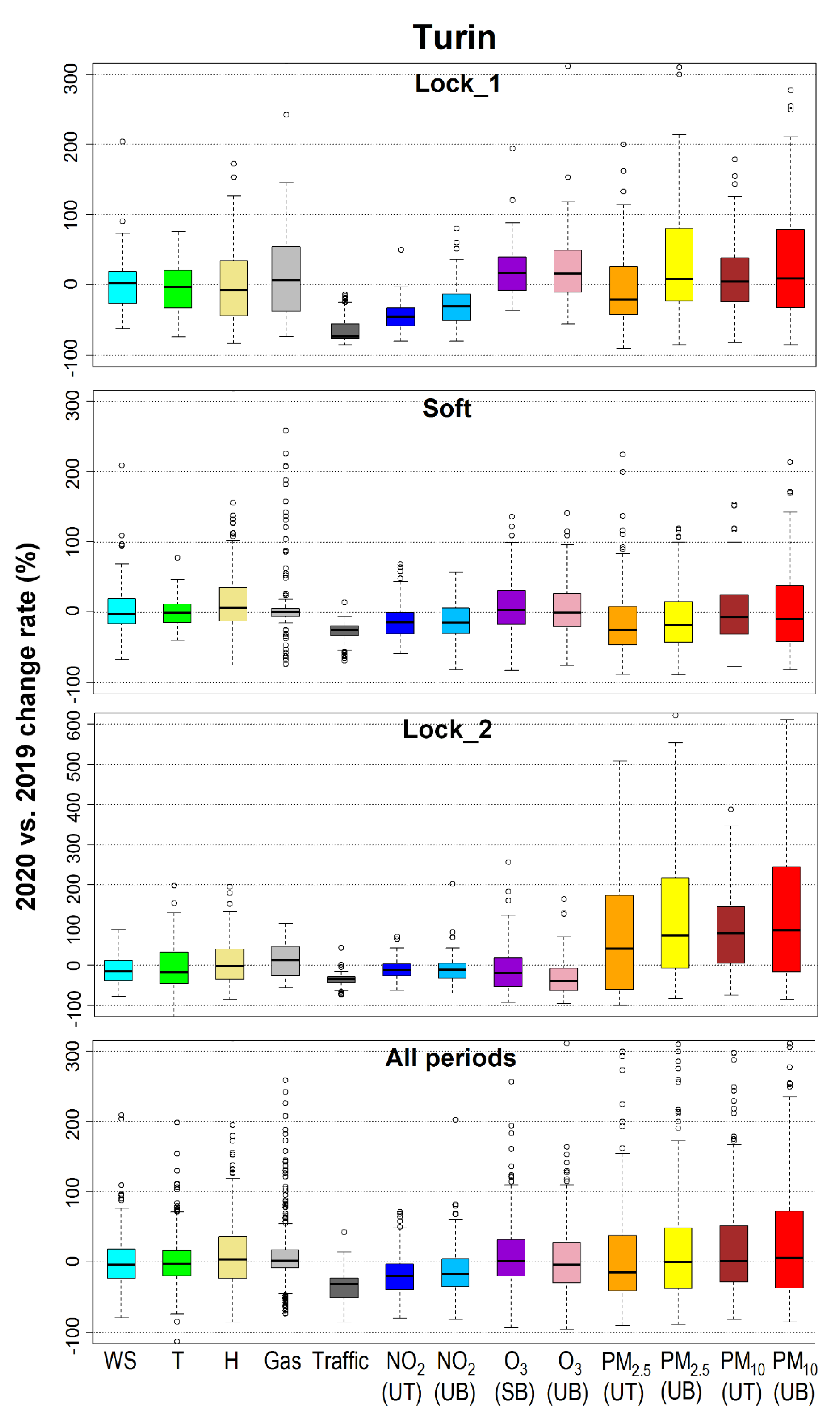
3.1. Turin
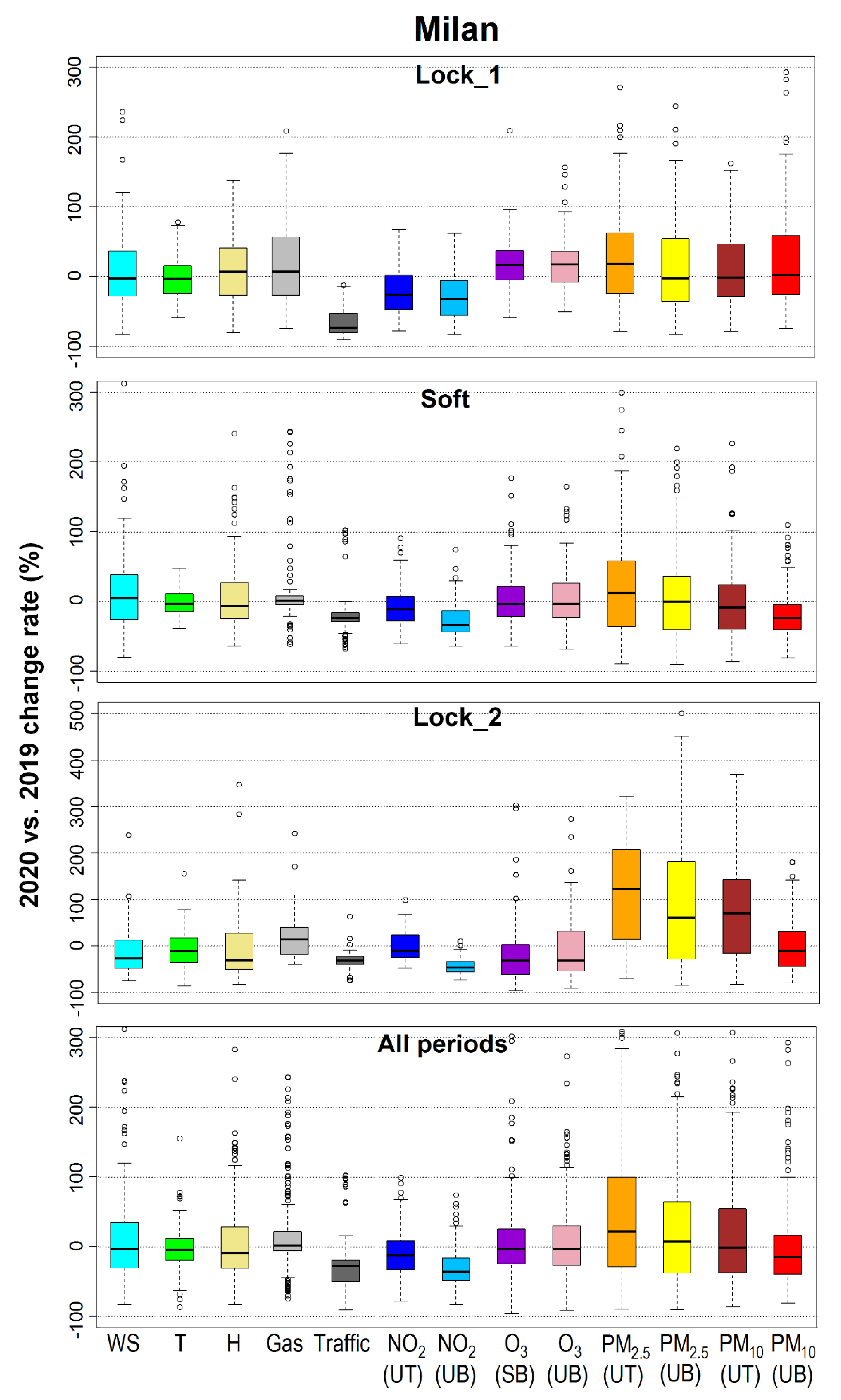
3.2. Milan
3.3. Bologna
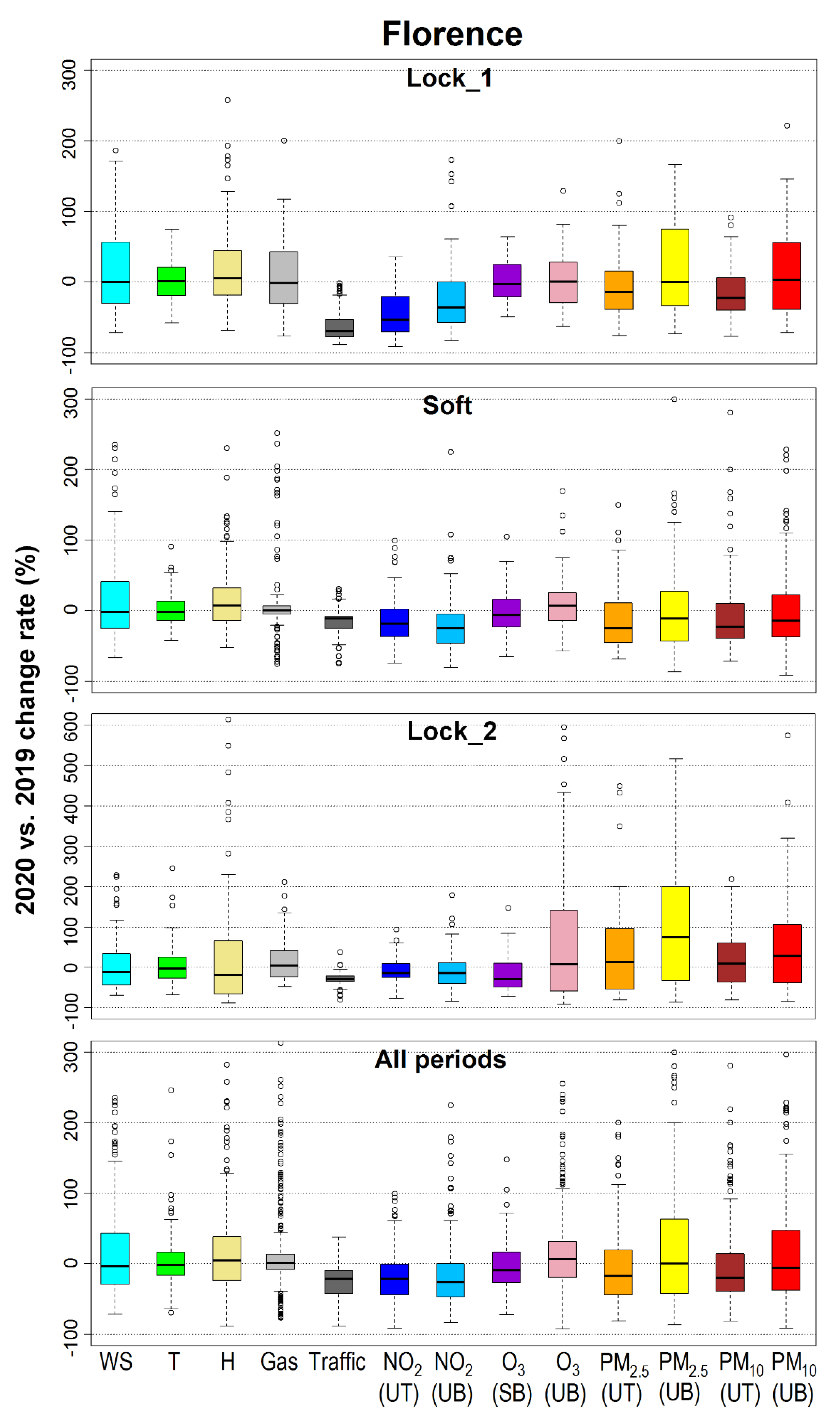
3.4. Florence
4. Discussion
4.1. Air Quality Pattern during the Three Periods
4.1.1. Lock_1
4.1.2. Soft
4.1.3. Lock_2
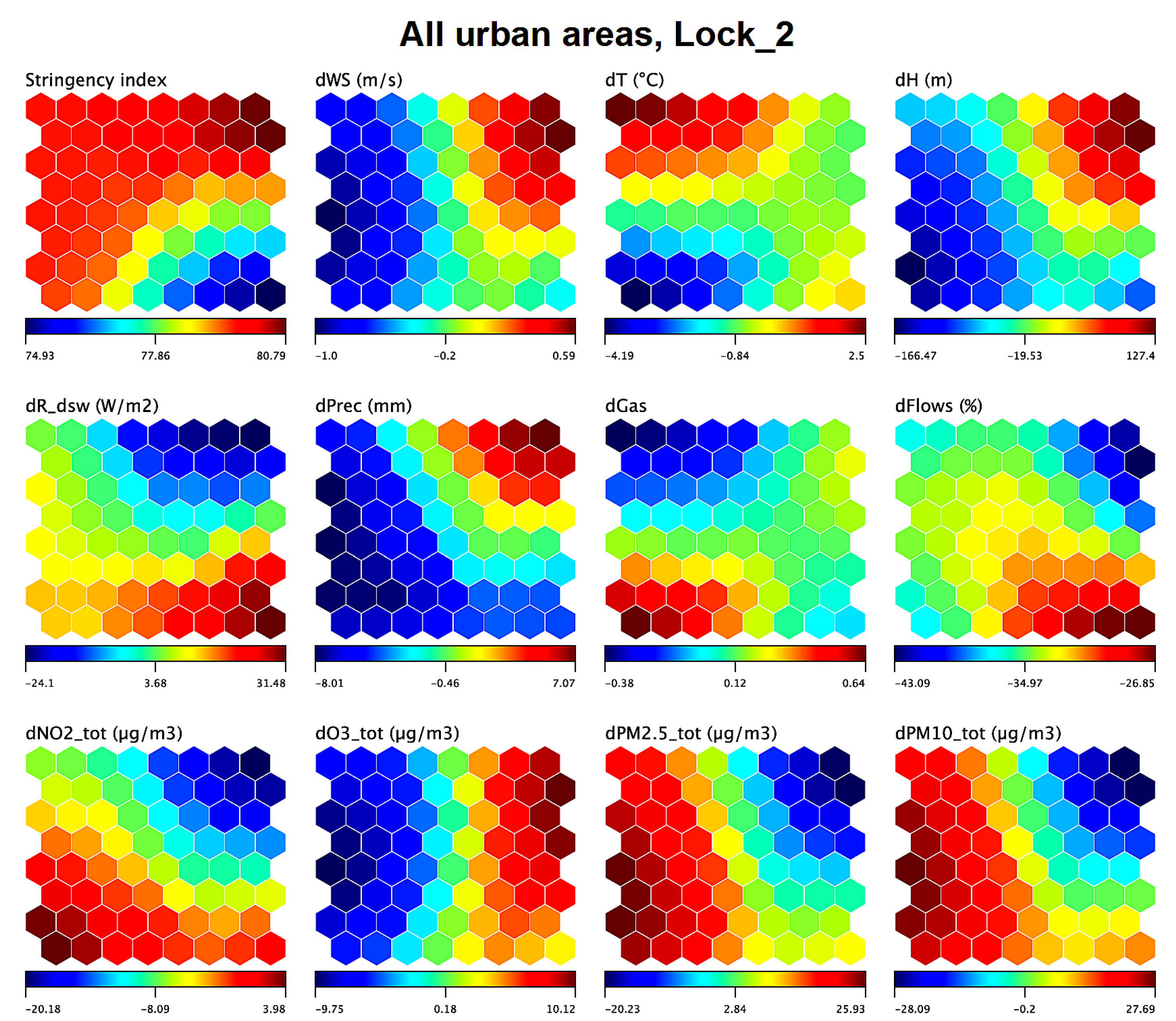
4.2. Further Insight into the Lock_2 Period
5. Conclusions
Supplementary Materials
Author Contributions
Funding
Institutional Review Board Statement
Informed Consent Statement
Data Availability Statement
Acknowledgments
Conflicts of Interest
References
- Sharifi, A.; Khavarian-Garmsir, A.R. The COVID-19 pandemic: Impacts on cities and major lessons for urban planning, design, and management. Sci. Total Environ. 2020, 749, 142391. [Google Scholar] [CrossRef] [PubMed]
- Gkatzelis, G.I.; Gilman, J.B.; Brown, S.S.; Eskes, H.; Gomes, A.R.; Lange, A.C.; McDonald, B.C.; Peischl, J.; Petzold, A.; Thompson, C.R.; et al. The global impacts of COVID-19 lockdowns on urban air pollution: A critical review and recommendations. Elem. Sci. Anth. 2021, 9, 00176. [Google Scholar] [CrossRef]
- Usman, M.; Ho, Y.S. COVID-19 and the emerging research trends in environmental studies: A bibliometric evaluation. Environ. Sci. Pollut. Res. 2021, 28, 16913–16924. [Google Scholar] [CrossRef]
- Casado-Aranda, L.A.; Sánchez-Fernández, J.; Viedma-del-Jesús, M.I. Analysis of the scientific production of the effect of COVID-19 on the environment: A bibliometric study. Environ. Res. 2021, 193, 110416. [Google Scholar] [CrossRef]
- Adam, M.G.; Tran, P.T.; Balasubramanian, R. Air quality changes in cities during the COVID-19 lockdown: A critical review. Atmos. Res. 2021, 264, 105823. [Google Scholar] [CrossRef] [PubMed]
- Donzelli, G.; Cioni, L.; Cancellieri, M.; Llopis-Morales, A.; Morales-Suárez-Varela, M. Relations between Air Quality and Covid-19 Lockdown Measures in Valencia, Spain. Int. J. Environ. Res. Public Health 2021, 18, 2296. [Google Scholar] [CrossRef]
- Cucciniello, R.; Raia, L.; Vasca, E. Air quality evaluation during COVID-19 in Southern Italy: The case study of Avellino city. Environ. Res. 2022, 203, 111803. [Google Scholar] [CrossRef]
- Pandey, M.; George, M.P.; Gupta, R.K.; Gusain, D.; Dwivedi, A. Impact of COVID-19 induced lockdown and unlock down phases on the ambient air quality of Delhi, capital city of India. Urban Clim. 2021, 39, 100945. [Google Scholar] [CrossRef]
- Sokhi, R.S.; Singh, V.; Querol, X.; Finardi, S.; Targino, A.C.; de Fatima Andrade, M.; Pavlovic, R.; Garland, R.M.; Massagué, J.; Kong, S.; et al. A global observational analysis to understand changes in air quality during exceptionally low anthropogenic emission conditions. Environ. Int. 2021, 157, 106818. [Google Scholar] [CrossRef]
- Akritidis, D.; Zanis, P.; Georgoulias, A.K.; Papakosta, E.; Tzoumaka, P.; Kelessis, A. Implications of COVID-19 Restriction Measures in Urban Air Quality of Thessaloniki, Greece: A Machine Learning Approach. Atmosphere 2021, 12, 1500. [Google Scholar] [CrossRef]
- Chen, L.W.A.; Chien, L.C.; Li, Y.; Lin, G. Nonuniform impacts of COVID-19 lockdown on air quality over the United States. Sci. Total Environ. 2020, 745, 141105. [Google Scholar] [CrossRef]
- Dantas, G.; Siciliano, B.; Franca, B.B.; da Silva, C.M.; Arbilla, G. The impact of COVID-19 partial lockdown on the air quality of the city of Rio de Janeiro, Brazil. Sci. Total Environ. 2020, 729, 139085. [Google Scholar] [CrossRef]
- Shakoor, A.; Chen, X.; Farooq, T.H.; Shahzad, U.; Ashraf, F.; Rehman, A.; Sahar, N.E.; Yan, W. Fluctuations in environmental pollutants and air quality during the lockdown in the USA and China: Two sides of COVID-19 pandemic. Air Qual. Atmos. Health 2020, 13, 1335–1342. [Google Scholar] [CrossRef] [PubMed]
- Gualtieri, G.; Brilli, L.; Carotenuto, F.; Vagnoli, C.; Zaldei, A.; Gioli, B. Quantifying road traffic impact on air quality in urban areas: A Covid19-induced lockdown analysis in Italy. Environ. Pollut. 2020, 267, 115682. [Google Scholar] [CrossRef] [PubMed]
- Pei, Z.; Han, G.; Ma, X.; Su, H.; Gong, W. Response of major air pollutants to COVID-19 lockdowns in China. Sci. Total Environ. 2020, 743, 140879. [Google Scholar] [CrossRef] [PubMed]
- Putaud, J.P.; Pozzoli, L.; Pisoni, E.; Dos Santos, S.M.; Lagler, F.; Lanzani, G.; Dal Santo, U.; Colette, A. Impacts of the COVID-19 lockdown on air pollution at regional and urban background sites in northern Italy. Atmos. Chem. Phys. 2021, 21, 7597–7609. [Google Scholar] [CrossRef]
- Wade, A.; Petherick, A.; Kira, B.; Tatlow, H.; Elms, J.; Green, K.; Hallas, L.; di Folco, M.; Hale, T.; Phillips, T.; et al. Variation in Government Responses to COVID-19. BSG-WP-2020/032, Version 13.0. March 2022. Available online: https://www.bsg.ox.ac.uk/research/publications/variation-government-responses-covid-19 (accessed on 7 June 2022).
- Kumar, S.; Managi, S. Does stringency of lockdown affect air quality? Evidence from Indian cities. Econ. Disasters Clim. Chang. 2020, 4, 481–502. [Google Scholar] [CrossRef]
- Dang, H.A.H.; Trinh, T.A. Does the COVID-19 lockdown improve global air quality? New cross-national evidence on its unintended consequences. J. Environ. Econ. Manag. 2021, 105, 102401. [Google Scholar] [CrossRef]
- Hersbach, H.; Bell, B.; Berrisford, P.; Hirahara, S.; Horányi, A.; Muñoz-Sabater, J.; Nicolas, J.; Peubey, C.; Radu, R.; Schepers, D.; et al. The ERA5 global reanalysis. Q. J. R. Meteorol. Soc. 2020, 146, 1999–2049. [Google Scholar] [CrossRef]
- Querol, X.; Massagué, J.; Alastuey, A.; Moreno, T.; Gangoiti, G.; Mantilla, E.; Duéguez, J.J.; Escudero, M.; Monfort, E.; García-Pando, C.P.; et al. Lessons from the COVID-19 air pollution decrease in Spain: Now what? Sci. Total Environ. 2021, 779, 146380. [Google Scholar] [CrossRef]
- Campanelli, M.; Iannarelli, A.M.; Mevi, G.; Casadio, S.; Diémoz, H.; Finardi, S.; Dinoi, A.; Castelli, E.; di Sarra, A.; Di Bernardino, A.; et al. A wide-ranging investigation of the COVID-19 lockdown effects on the atmospheric composition in various Italian urban sites (AER–LOCUS). Urban Clim. 2021, 39, 100954. [Google Scholar] [CrossRef]
- Hale, T.; Angrist, N.; Goldszmidt, R.; Kira, B.; Petherick, A.; Phillips, T.; Webster, S.; Cameron-Blake, E.; Hallas, L.; Majumdar, S.; et al. A Global Panel Database of Pandemic Policies (Oxford COVID-19 Government Response Tracker). Nat. Hum. Behav. 2021, 5, 529–538. [Google Scholar] [CrossRef] [PubMed]
- Blavatnik School of Government, University of Oxford. Oxford COVID-19 Government Response Tracker. Available online: https://github.com/OxCGRT/covid-policy-tracker/blob/master/data/timeseries/stringency_index.csv (accessed on 7 June 2022).
- ECMWF Reanalysis v5 (ERA5). Available online: https://www.ecmwf.int/en/forecasts/dataset/ecmwf-reanalysis-v5 (accessed on 7 June 2022).
- ISPRA. Comparison between Energy Consumption and Heating Degree Days (HDD). Projections to 2050 of HDD in different climate scenarios. Report 277/2017. December 2017. Available online: https://www.isprambiente.gov.it/en/publications/reports/comparison-between-energy-consumption-and-heating-degree-days-hdd-.-projections-to-2050-of-hdd-in-different-climate-scenarios (accessed on 7 June 2022).
- Gualtieri, G.; Carotenuto, F.; Finardi, S.; Tartaglia, M.; Toscano, P.; Gioli, B. Forecasting PM10 hourly concentrations in northern Italy: Insights on models performance and PM10 drivers through self-organizing maps. Atmos. Pollut. Res. 2018, 9, 1204–1213. [Google Scholar] [CrossRef]
- 5T srl. Traffic Flow Open Data. Available online: http://aperto.comune.torino.it/dataset/flussi-di-traffico (accessed on 7 June 2022). (In Italian).
- Municipality of Milan. Open data. Available online: http://dati.comune.milano.it (accessed on 7 June 2022). (In Italian).
- Municipality of Bologna. Mobility Open Data. Available online: https://opendata.comune.bologna.it/explore/dataset/bologna-daily-mobility/information (accessed on 7 June 2022). (In Italian).
- Snap4City. Traffic Flow Data in Florence. Available online: https://www.snap4city.org/dashboardSmartCity/view/index.php?iddasboard=MTE5MQ (accessed on 7 June 2022).
- ARPA Piedmont. IREA Regional Emission Inventory—2015 Emissions in the Piedmont Region. Available online: http://www.sistemapiemonte.it/fedwinemar/elenco.jsp (accessed on 7 June 2022). (In Italian).
- ARPA Lombardy. INEMAR Regional Emission Inventory—2017 Emissions in the Lombardy Region. Available online: https://www.inemar.eu/xwiki/bin/view/InemarDatiWeb/Aggiornamenti+dell%27inventario+2017 (accessed on 7 June 2022). (In Italian).
- ARPA Emilia-Romagna. INEMAR Regional Emission Inventory—2017 Emissions in the Emilia-Romagna Region. Available online: https://datacatalog.regione.emilia-romagna.it/catalogCTA/dataset/inventario-regionale-emissioni-in-atmosfera-inemar/resource/2e223430-b917-4e8f-a6ea-27f2a44cfac5 (accessed on 7 June 2022). (In Italian).
- Tuscany Region. IRSE Regional Emission Inventory. Available online: https://www.regione.toscana.it/-/inventario-regionale-sulle-sorgenti-di-emissione-in-aria-ambiente-irse (accessed on 7 June 2022). (In Italian).
- ISPRA. Ammonia Emissions from the Agricultural Sector. Available online: https://annuario.isprambiente.it/pon/basic/44 (accessed on 7 June 2022). (In Italian).
- R Core Team. The R Project for Statistical Computing. Available online: https://www.r-project.org (accessed on 7 June 2022).
- R Graphics Package. Available online: https://stat.ethz.ch/R-manual/R-devel/library/graphics/html/00Index.html (accessed on 7 June 2022).
- Kohonen, T. Self-Organizing Maps, 2nd ed.; Springer: Heidelberg, Germany, 2001. [Google Scholar]
- ANAS. Osservatorio del Traffico—Dati di Riferimento Marzo 2020. April 2020. Available online: https://www.stradeanas.it/sites/default/files/SMI4%20-%20Osservatorio%20del%20Traffico%20Marzo%202020.pdf (accessed on 7 June 2022). (In Italian).
- ANAS. Osservatorio del Traffico—Dati di Riferimento Aprile 2020. May 2020. Available online: https://www.stradeanas.it/sites/default/files/SMI4%20-%20Osservatorio%20del%20Traffico%20Aprile%202020.pdf (accessed on 7 June 2022). (In Italian).
- Rossi, R.; Ceccato, R.; Gastaldi, M. Effect of road traffic on air pollution. Experimental evidence from COVID-19 lockdown. Sustainability 2020, 12, 8984. [Google Scholar] [CrossRef]
- Gaubert, B.; Bouarar, I.; Doumbia, T.; Liu, Y.; Stavrakou, T.; Deroubaix, A.; Darras, S.; Elguindi, N.; Granier, G.; Lacey, F.; et al. Global changes in secondary atmospheric pollutants during the 2020 COVID-19 pandemic. J. Geophys. Res. Atmos. 2021, 126, e2020JD034213. [Google Scholar] [CrossRef]
- Petit, J.E.; Dupont, J.C.; Favez, O.; Gros, V.; Zhang, Y.; Sciare, J.; Simon, L.; Truong, F.; Bonnaire, N.; Amodeo, T.; et al. Response of atmospheric composition to COVID-19 lockdown measures during spring in the Paris region (France). Atmos. Chem. Phys. 2021, 21, 17167–17183. [Google Scholar] [CrossRef]
- Patti, S.; Pillon, S.; Intini, B.; Susanetti, L.; Francescato, V.; Rossi, D. Survey to Estimate Woody Biomasses Consumption in Households. Action D3. Residential Wood Consumption Estimation in the Po Valley. Project PREPAIR (LIFE 15 IPE IT 013). 1 February 2020. Available online: http://www.lifeprepair.eu/?smd_process_download=1&download_id=8196 (accessed on 7 June 2022).
- Thunis, P.; Clappier, A.; Beekmann, M.; Putaud, J.P.; Cuvelier, C.; Madrazo, J.; de Meij, A. Non-linear response of PM2.5 to changes in NOx and NH3 emissions in the Po basin (Italy): Consequences for air quality plans. Atmos. Chem. Phys. 2021, 21, 9309–9327. [Google Scholar] [CrossRef]
- ARPA Lombardy. Valutazione Emissiva e Modellistica di Impatto sulla Qualità dell’Aria durante l’Emergenza COVID-19: Periodo Febbraio–Maggio. October 2020. Available online: https://www.arpalombardia.it/sites/DocumentCenter/Documents/Aria%20-%20Relazioni%20approfondimento/Emis-mod-report-stima-emissiva-COVID-19-lombardia_maggio20.pdf (accessed on 7 June 2022). (In Italian).
- Huang, X.; Ding, A.; Gao, J.; Zheng, B.; Zhou, D.; Qi, X.; Tang, R.; Wang, J.; Ren, C.; Nie, W.; et al. Enhanced secondary pollution offset reduction of primary emissions during COVID-19 lockdown in China. Natl. Sci. Rev. 2021, 8, nwaa137. [Google Scholar] [CrossRef]
- ARPA Lombardy. Gli Effetti dei Provvedimenti di Limitazione delle Attività sulle Concentrazioni di PM2.5 e sulla Composizione del PM10. Available online: https://www.arpalombardia.it/sites/DocumentCenter/Documents/Aria%20-%20Relazioni%20approfondimento/PM2.5-COVID_210318.pdf (accessed on 7 June 2022). (In Italian).
- Vesanto, J.; Alhoniemi, E. Clustering of the self-organizing map. IEEE Trans. Neural Netw. 2000, 11, 586–600. [Google Scholar] [CrossRef]
- Holst, J.; Mayer, H.; Holst, T. Effect of meteorological exchange conditions on PM10 concentration. Meteorol. Z. 2008, 17, 273–282. [Google Scholar] [CrossRef] [Green Version]
- Barmpadimos, I.; Hueglin, C.; Keller, J.; Henne, S.; Prévôt, A.S.H. Influence of meteorology on PM10 trends and variability in Switzerland from 1991 to 2008. Atmos. Chem. Phys. 2011, 11, 1813–1835. [Google Scholar] [CrossRef] [Green Version]
- Invernizzi, G.; Ruprecht, A.; Mazza, R.; De Marco, C.; Močnik, G.; Sioutas, C.; Westerdahl, D. Measurement of black carbon concentration as an indicator of air quality benefits of traffic restriction policies within the ecopass zone in Milan, Italy. Atmos. Environ. 2011, 45, 3522–3527. [Google Scholar] [CrossRef]
- Cai, H.; Xie, S. Traffic-related air pollution modeling during the 2008 Beijing Olympic Games: The effects of an odd-even day traffic restriction scheme. Sci. Total Environ. 2011, 409, 1935–1948. [Google Scholar] [CrossRef] [PubMed]
- Gualtieri, G.; Toscano, P.; Crisci, A.; Di Lonardo, S.; Tartaglia, M.; Vagnoli, C.; Zaldei, A.; Gioli, B. Influence of road traffic, residential heating and meteorological conditions on PM10 concentrations during air pollution critical episodes. Environ. Sci. Pollut. Res. 2015, 22, 19027–19038. [Google Scholar] [CrossRef]
- Duque, L.; Relvas, H.; Silveira, C.; Ferreira, J.; Monteiro, A.; Gama, C.; Rafael, S.; Freitas, S.; Borrego, C.; Miranda, A. Evaluating strategies to reduce urban air pollution. Atmos. Environ. 2016, 127, 196–204. [Google Scholar] [CrossRef]


Publisher’s Note: MDPI stays neutral with regard to jurisdictional claims in published maps and institutional affiliations. |
© 2022 by the authors. Licensee MDPI, Basel, Switzerland. This article is an open access article distributed under the terms and conditions of the Creative Commons Attribution (CC BY) license (https://creativecommons.org/licenses/by/4.0/).
Share and Cite
Gualtieri, G.; Brilli, L.; Carotenuto, F.; Vagnoli, C.; Zaldei, A.; Gioli, B. Long-Term COVID-19 Restrictions in Italy to Assess the Role of Seasonal Meteorological Conditions and Pollutant Emissions on Urban Air Quality. Atmosphere 2022, 13, 1156. https://doi.org/10.3390/atmos13071156
Gualtieri G, Brilli L, Carotenuto F, Vagnoli C, Zaldei A, Gioli B. Long-Term COVID-19 Restrictions in Italy to Assess the Role of Seasonal Meteorological Conditions and Pollutant Emissions on Urban Air Quality. Atmosphere. 2022; 13(7):1156. https://doi.org/10.3390/atmos13071156
Chicago/Turabian StyleGualtieri, Giovanni, Lorenzo Brilli, Federico Carotenuto, Carolina Vagnoli, Alessandro Zaldei, and Beniamino Gioli. 2022. "Long-Term COVID-19 Restrictions in Italy to Assess the Role of Seasonal Meteorological Conditions and Pollutant Emissions on Urban Air Quality" Atmosphere 13, no. 7: 1156. https://doi.org/10.3390/atmos13071156