Article

Performance Evaluation of the RANS Models in Predicting the Pollutant Concentration Field within a Compact Urban Setting: Effects of the Source Location and Turbulent Schmidt Number

by
Mohammad Reza Kavian Nezhad
*,
Carlos F. Lange
and
Brian A. Fleck
Department of Mechanical Engineering, University of Alberta, Edmonton, AB T6G 1H9, Canada
*
Author to whom correspondence should be addressed.
Atmosphere 2022, 13(7), 1013; https://doi.org/10.3390/atmos13071013
Submission received: 14 May 2022 / Revised: 17 June 2022 / Accepted: 20 June 2022 / Published: 23 June 2022
(This article belongs to the Special Issue Computational Fluid Dynamics Simulations of Urban Airflow)

Abstract

:
Computational Fluid Dynamics (CFD) is used to accurately model and predict the dispersion of a passive scalar in the atmospheric wind flow field within an urban setting. The Mock Urban Setting Tests (MUST) experiment was recreated in this work to test and evaluate various modeling settings and to form a framework for reliable representation of dispersion flow in compact urban geometries. Four case studies with distinct source locations and configurations are modeled using Reynolds-Averaged Navier–Stokes (RANS) equations with ANSYS CFX. The performance of three widely suggested closure models of standard k ε , RNG k ε , and SST k ω is assessed by calculating and interpreting the statistical performance metrics with a specific emphasis on the effects of the source locations. This work demonstrates that the overprediction of the turbulent kinetic energy by the standard k ε counteracts the general underpredictions by RANS in geometries with building complexes. As a result, the superiority of the standard k ε in predicting the scalar concentration field over the two other closures in all four cases is observed, with SST k ω showing the most discrepancies with the field measurements. Additionally, a sensitivity study is also conducted to find the optimum turbulent Schmidt number ( S c t ) using two approaches of the constant and locally variable values.

1. Introduction

Statistical studies show a significant soar in the urban population in recent years, with a prediction that around 70% of the earth’s population will be living in urban regions over the next few decades [1]. This sudden surge in urbanization has come with detrimental impacts on urban air quality caused by airborne pollutants emitting from various sources. In this regard, acquiring a thorough understanding of how these pollutants are dispersed in the presence of structural obstacles with varying shapes and dimensions is essential to effectively maintain the air quality at acceptable levels. For this purpose, urban planners have used analytical and semi-empirical dispersion models to assess the pollutant distribution field [2,3]. However, using these dispersion models, which were mostly developed based on very idealized generalizations of the meteorological conditions and simplified geometrical topographies, leads to extremely conservative and less energy-efficient guidelines in the design [4,5,6,7].
Computational Fluid Dynamics (CFD) can be introduced as a reliable alternative method to predict the dispersion pattern in complex turbulent flow fields [8]. It is generally less costly than experiments, provides flow estimates at every point in the computational domain, and can predict the concentration field more accurately than the analytical and semi-empirical models [9]. However, the highly complex nature of the turbulent flow in the Atmospheric Boundary Layer (ABL) demands simplifications and assumptions in every step of modeling. Special considerations are required to implement a suitable numerical algorithm and carefully define grid resolution, boundary conditions, wall functions, and other modeling settings [10,11,12]. Additionally, CFD models must be validated by comparison with high-quality experimental measurements to assess the severity of the introduced errors and uncertainties [13]. Tracer gas experiments can produce valuable data to validate the open field dispersion CFD models [14,15,16]. Nevertheless, there are high costs and challenges associated with conducting such tracer experiments in urban regions, which makes it impractical to acquire a reliable dataset in every geometry with each unique domain topography and diverse structural arrangement [17,18,19]. In this regard, introducing a well-tested and improved infrastructure is considerably beneficial in setting the guidelines for a reliable and efficient practice in numerical prediction of pollutant dispersion in analogous cases.
Attempts have been made in recent years to perfect the numerical modeling of atmospheric dispersion flows in simplified geometries (e.g., isolated buildings, the street canyon between two buildings, flat terrain, etc.) [20,21,22,23,24]. However, many studies have pointed out the unique and considerable impacts of the neighboring buildings and urban morphologies on the wind and dispersion fields and emphasized the importance of these types of investigations [18,25,26]. Despite the endeavor made by previous researchers, precise prediction of the pollutant concentration field and dispersion in high-density urban settings remains very challenging. This is due to the behavior of the turbulent flows with large-scale recirculation structures and three-dimensional strain fields that challenge turbulence models. In this regard, contributing to the “Best-Practice” in simulating the ABL dispersion flow within compact urban settings is set as the primary goal of this research paper.
One of the most critical decisions that needs to be made by the modeler is selecting a suitable physical model to recreate the flow field in the regions of interest. Considering the well-established balance of the Reynolds-Averaged Navier–Stokes (RANS) model between the computational cost and the prediction accuracy, this approach has been extensively suggested for atmospheric dispersion, where the mean quantities of the flow characteristics are studied [27,28]. A wide variety of turbulence models are proposed in the literature to estimate the turbulent viscosity resulting from the Boussinesq hypothesis and to close the RANS equations [29]. Properly selecting the closure model can immensely impact the quality and efficiency of the predictions. Therefore, it is considered an essential step in contributing to the “Best-Practice” in CFD modeling of the near-field pollutant dispersion.
Narjisse et al., evaluated the capability of the standard k ε and Shear Stress Transport (SST) k ω in accurately resolving the wind flow in the presence of a hilly terrain [30]. They concluded that even though standard k ε overpredicted the wind velocity near the wall, it was still a more reasonable choice for modeling the flow for these geometries than SST k ω which offered slightly better predictions at a much higher computational cost. Tominaga et al., also tested the performance of several RANS closures in modeling the atmospheric wind flow with results of the unsteady simulations and showed that RNG k ε provided a comparatively accurate representation of the flow around the building [31]. However, the results were only validated for a case of an isolated high-rise building, and a general conclusion could not be drawn for more complicated situations of complex urban geometries. Hosseinzadeh et al., performed a series of validation studies on CFD models of wind flow between two buildings and examined standard k ε , realizable k ε , standard k ω , SST k ω closure models [32]. They found that k ε based models predicted more accurate results for this configuration compared with of k ω based models, with standard k ε performing slightly better overall.
The selection of a proper closure model to represent the wind and turbulence fields becomes even more crucial in cases of accurately modeling the pollutant dispersion flows. Lateb et al., carried out a comparison study by simulating the dispersion flow between two buildings of different heights using three types of k-ε turbulence models to find the proper selection for the geometry configuration of his study [33]. They observed that the realizable model produced more accurate results in cases with lower stacks’ momentum ratios and eights, while RNG performed better for other cases. An et al., numerically modeled the dispersion of a pollutant emitting from a ground-level source around a single-block building to build a validation case. The SST k ω was used, and comparison with wind tunnel data demonstrated the satisfactory performance of this closure model [34]. However, a systematic comparison with other closure models was missing to indicate whether SST k ω was the best possible choice for this case or not. Keshavarzian et al., studied the effects of the pollutant source location (different heights on the building sidewall) on the dispersion pattern by numerically simulating flow around an isolated high-rise building [35]. They only validated the standard k ε closure model in this paper, and therefore it is not clear how the location of the source might affect the performance of the closure models and the overall prediction of the concentration field.
Several other studies also evaluated the performance of various turbulence models in modeling the atmospheric dispersion flow in different geometries [36,37,38,39]. The fact that each turbulence model provides relatively different predictions in each geometry justifies carrying out this sensitivity study as an essential step of this research to understand each model’s limitations and further contribute to the “Best-Practice” in urban dispersion modeling. Additionally, the type of the pollutant source location (ground-level sources upstream or downstream of an obstacle, sources in urban canopies, rooftop sources, etc.) is another factor that might impact the accuracy of the results generated by each turbulence model [40]. In this regard, to address the gap in the literature, three of the most commonly used models in computational wind engineering ([41]), including standard k ε , RNG k ε , and SST k ω , have been chosen to be comparatively analyzed in the context of the compact urban-like geometries. Four different case studies from the detailed and thorough Mock Urban Setting Tests (MUST) dispersion dataset have been selected that provide four distinct types of source locations.
The turbulent Schmidt number ( S c t ) is another influencing parameter in atmospheric dispersion modeling that needs to be tested and modified for benchmarking the “Best-Practice”. Despite the proven profound effects of S c t , there is no clear definition of this parameter, and most previous studies used a constant value in the broad range of 0.2–1.3, depending on the specific flow properties and geometry of the problem [42]. The common approach for determining the optimum S c t suggests conducting a series of validation studies beforehand to test different values [6,43,44]. In this paper, in addition to the conventional method of finding the optimum and constant value of S c t , the method of using a variable S c t will be also tested in context of the dispersion modeling in a complex urban geometry.

2. Fundamentals and Governing Equations

The pattern in which an emitted pollutant plume will be dispersed in the atmosphere is dependent on the wind regime and turbulence. Wind flow in a compact urban setting is disturbed by the presence of structural features such as buildings of various heights and shapes and by natural landscapes, which form a wind profile that is quite distinct from the ones in the open rural area. As this work aims to model the dispersion of the emitting plume from sources within an urban setting, a quick overview of the governing equations and methodology is beneficial to justify the applicable assumptions.
The mass, momentum, and energy conservation laws can be applied in the form of Navier–Stokes equations to govern the dynamics of ABL flow. Assuming an isothermal fluid flow in a neutral atmosphere, the energy equation will not be used in the context of this study. The remaining governing equations are simplified by considering the applicable assumptions, such as steady-state, incompressible airflow, and constant isotropic viscosity. Since the region of interest in this study is limited to the inner sublayer of the ABL, the terrestrial Coriolis effects can also be neglected [45]. To further evaluate the validity of this assumption, the non-dimensionalized Rossby number ( R o ) was estimated. R o is defined as the ratio of the inertial forces to the Coriolis forces and can be expressed as [46]:
R o = U L f
where U is the characteristic horizontal velocity, L is the characteristic horizontal length scale, and f is the Coriolis frequency. Considering that the order of magnitudes of these parameters in this research are U ~ 1 , L ~ 10 2 , and f ~ 10 5 , the resulting R o is of the order of 10 3 which justifies the assumption of negligible Coriolis effects.
Large length scales caused by the available structures, as well as the typical wind speeds of interest in these types of studies, will result in the Reynolds number being the order of 10 6 10 8 . Therefore, the airflow and pollutant dispersion in the ABL will have a rich turbulent nature. In this work, the dispersion of the pollutant scalar in the complex urban geometry is investigated that is being continuously released from the source points. Therefore, considering the large size of the computational domain and the interest in the mean quantities of flow characteristics, the RANS method has been chosen to solve the governing equations. Using the Reynolds decomposition, the continuity and momentum equations can be presented in their time-averaged forms as follows:
u ¯ i x i = 0
u ¯ j u ¯ i x j = 1 ρ p ¯ x i + ν 2 u ¯ i x j 2 u i u j ¯ x j
where u ¯ i and u i . are the time-averaged and the fluctuating fluid velocity in the three ( i , j , k ). Cartesian directions, x i denotes these directions, ρ is the density, and p is the pressure. On the right-hand side of Equation (3), the introduced turbulent term is the time-averaged Reynold stress tensor ( u i u j ¯ ) which contributes to the convective momentum transfer due to the turbulent eddies. With the use of the Boussinesq approximation, the Reynolds stress term in Equation (3) is modeled as:
ρ u i u j ¯ = 2 μ t S i j 1 3 u ¯ k x k δ i j 2 3 ρ k δ i j
where μ t is the turbulence viscosity, k = 0.5 u i u i ¯ is the turbulence kinetic energy per unit mass, S i j = 1 / 2 u ¯ i / x j + u ¯ j / x i is the shear strain rate, and δ i j is the Kronecker delta. It should be noted that although the molecular viscosity, μ , is a property of the fluid, the turbulence viscosity is considered to be a property of the flow [40]. Considering the number of unknowns in Equations (2)–(4) for solving the flow field, supplementary equations are required to close the problem, which are provided through the available closure models.
The Menter SST k ω has been considered as one of the possible choices in this research paper, following the success of implementing this model in similar research work [47]. SST k ω is introduced as a hybrid turbulence model by providing a transformation from the k ε into a k ω model in the near-wall regions and using the standard k ε model in the fully turbulent regions of the geometry far from the wall [48]. The Standard k ε and RNG k ε closure models have been selected along with the SST k ω for further evaluation of their performance in predicting the mean concentration field in a compact urban-like geometry. Detailed descriptions of the mentioned closure models can be found in the ANSYS CFX user guide [49].
The different turbulence models also require case-specific modifications in the meshing procedure since the appropriate wall treatment heavily depends on it. One of the advantages of the SST k ω model is that it directly resolves the viscous sublayer. Even though the accurate reproduction of the separation and recirculation zones can be achieved using this model, extra refinement is necessary adjacent to the wall, which could considerably increase the computational expenses. The k ε based models, on the other hand, utilize the wall functions to resolve flow near the surfaces, which, by comparison, reduces the computational cost and the modeling complexities [41]. However, this could lead to a poor prediction of viscous effects near the walls, leading to the inaccurate prediction of the pollutant dispersion in cases where the source is located near the ground or on the roofs. In this regard, a careful investigation of the overall performance of the selected turbulence models is necessary to benchmark the recommended practice for modeling the dispersion of pollutants emitting from different types of source locations. In this paper, the widely used scalable wall function will be tested to resolve the flow adjacent to the wall when considering the k ε based models [49].
Furthermore, the governing equations are supplemented with the Eulerian diffusion-advection equation. With the flow field and the turbulent characteristics solved, the mass fraction of the scalar (pollutant) needs to be decomposed into mean, C , and the fluctuating, c , components. The turbulent scalar fluxes, c u j ¯ , can be estimated as D t C / x j assuming the standard gradient diffusion hypothesis (SGDH). D t is the turbulence mass diffusivity and is defined as the ratio of turbulence viscosity ( v t ) to the turbulence Schmidt number ( S c t ). Numerous studies have demonstrated the profound influence of the S c t on the turbulent diffusion, which drastically affects the predicted concentration field by RANS equations. Employing the SGDH, the transport equation can be expressed as:
u j C x j = D + D t 2 C x i x i + S
where D is the molecular diffusion coefficient for the pollutant in the airflow field, and S represents the scalar source term. The pollutant is assumed as a passive scalar, meaning that due to its low mass fraction in the field and its non-reactive nature, its concentration does not affect the urban flow field. Therefore, the scalar transport equation can be solved after the flow field is resolved.
To effectively make a comparison between the numerical and experimental results, the non-dimensionalized concentration parameter ( C * ) defined by Equation (6) is used hereafter, where C is the mean concentration in ppm at a given location in the domain, U is the mean upstream wind velocity in m / s , H is an arbitrary characteristic length in m , and Q is the source’s volumetric flowrate in m 3 / s . Using the C * , the plume concentration field and its lateral and vertical spreads in various case studies can be compared quantitively to draw appropriate conclusions at any wind speed and discharge flow rates.
C * = 10 6 C U H 2 Q

3. Description of Case Studies

The comprehensive dispersion dataset of the MUST experiments has been selected to evaluate the modeling method and test several modeling settings that have the most profound effects on the accuracy of the predictions. The MUST tracer study refers to a series of tests conducted in an urban-like setting with the primary purpose of providing a valuable resource that includes the meteorological and dispersion data, suitable for validating the accuracy of the dispersion models and CFD simulations [50,51,52,53,54]. In this experimental setup, a 10 by 12 array of shipping containers was placed outdoors in the center of the test domain over relatively flat ground. The containers were 12.2 m long ( L ), 2.4 m wide ( W ), and 2.5 m high ( H ), forming an approximately 200 m × 200 m square array (Figure 1a). Propylene was used as the tracer gas in this experiment, and six different release configurations (with assigned letters A to F) were considered to cover a wide variety of cases (Figure 1b). In total, 68 trials were performed: 63 with continuous releases and 5 with puff releases. The source locations varied from positions within or upwind of the test array (37 locations).
The horizontal concentration field was measured using 40 Digital Photoionization Detectors (dPID) located in four parallel lines downstream of the source at the height of 1.6 m. The horizontal sampling lines are named as Lines 1–4 (Figure 1a). The vertical concentration field was mapped using 8 dPIDs installed on the central tower at various heights, and 6 Ultra Violet Ion Collectors (UVIC) installed on each of the four 6 m towers. Since the climatological analysis suggested that the test region frequently experiences wind flow coming from the two directions of Southeast and Northwest, two 16 m masts were also installed, approximately 30 m Southeast and Northwest of the array, to capture flow characteristics upstream and downstream.
In an attempt to collect data in neutral and stable atmospheric conditions, 15 min trials were done mainly in the early mornings or nights when surface cooling takes place in the absence of sun [55]. During these periods, the ground generally cools more quickly than its surrounding air due to radiation, resulting in a temperature gradient less negative than the adiabatic lapse rate that suppresses the vertical mixing. However, in the presence of a strong wind, nocturnal stability can be diminished by the turbulent mixing, which results in a temperature gradient closer to neutral conditions. The uncontrolled nature of the boundary conditions in field experiments results in the instantaneous variation of the measurements, making it quite challenging to use the generated data to validate quasi steady-state numerical models based on Reynolds averaging. In this regard, Yee ([56]) further processed the dataset and extracted 200 s in each trial with the least recorded variation in the upstream flow that could be considered quasi-steady periods.
Considering the number of available test cases in the MUST dataset, a careful assessment of all the 68 trials was necessary to define the appropriate case studies. The selected cases should contain high-quality measurements, be consistent with the assumptions, and represent diverse scenarios to enrich the outcomes of this paper. In this regard, only trials with continuous tracer gas release were considered, and cases with puff releases were disregarded. The state of atmospheric stability during the remaining trials is another important factor that should be considered for selecting the target case studies. The Obukhov length ( L O ) has been shown to be a practical scale in determining the level of atmospheric stability [24,57]. Considering the assumption of the neutral atmospheric conditions in this work, the ideal choice was to use the measurements from the trials conducted in similar stability states. In this regard, the number of possible case studies is further limited to tests with positive and large L O to account for neutral and near stable conditions.
The height and the location type of the source point are considered to be the final criterion needed to select trials that assure diverse situations for comparatively assessing the turbulence closure models. For the purpose of this study, four distinct source location types were selected (Figure 1b):
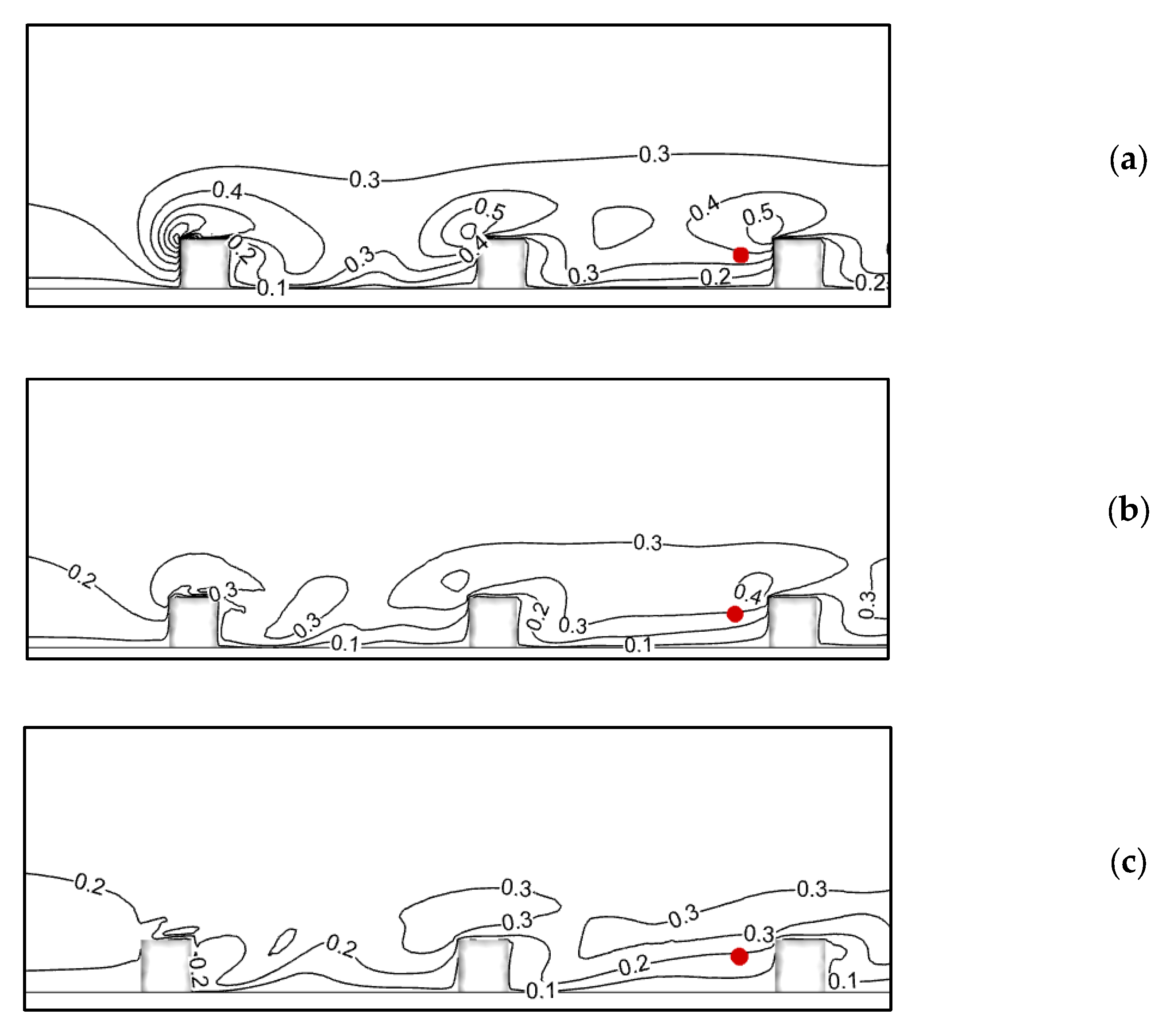
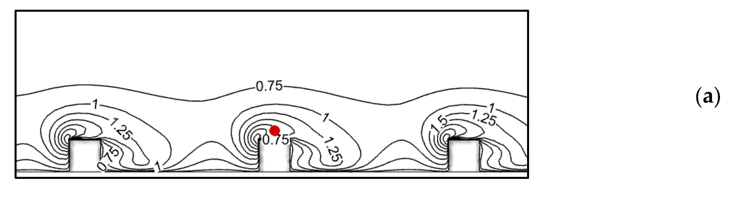
  • Source type A: located 1 m upstream of container J3 within the array ( z / H = 0.72 ).
  • Source type D: located on the rooftop of container J9 within the array ( z / H = 1.04 ).
  • Source type E: located 24 m upstream of container L1 outside the array ( z / H = 0.52 ).
  • Source type F: located on the road, centered between containers K8 and L8 long sides ( z / H = 0.72 ).
The final four case studies are shown in Table 1 with all the necessary quantities (mean calculated values during the 200 s of quasi-steady period) required for accurately modeling the dispersion flow. The quantities presented in Table 1 are the tracer release rate ( q s ), the source location type, the source height ( Z s ), the upstream wind speed at 4 m height ( S 04 ), the upstream wind direction at 4 m height with a positive angle measured counter-clockwise from the y-axis ( α 04 ). The friction velocity ( u τ ), Obukhov length ( L O ), and the turbulence kinetic energy ( k ) are also calculated at 4 m height on the central tower.

4. CFD Model Description

4.1. General Settings

The ANSYS CFX software was used to model the passive scalar dispersion of the MUST experiments by discretizing the RANS equations described previously. Deciding on the size and shape of the computational domain was the first step toward setting up a reliable framework for modeling the dispersion flow. Rectangular computational domains were selected for our simulations, having the inlet and outlet planes perpendicular to the free stream. Following guidelines recommended by Franke et al. [58], the distance from the inlet, lateral, and top boundary to the building cluster should be at least 5 H , while a minimum distance of 10 H should be considered to the outlet ( H represents the height of the tallest obstacle within the geometry). Having these criteria in mind and testing different arrangements, the size of the computational domain in this research was extended ( 14 H from the inlet, 10 H from lateral, 12 H from top boundaries, and 20 H from the outlet) to ensure that no backflow at the boundaries hampered the convergence of the iterative solver. Considering the size of the MUST array and the maximum height of the obstacles within ( H = 2.5   m ), a nested computational domain with an inner domain of 200   m × 200   m × 10   m and outer domain of 285   m × 250   m × 32.5   m was defined.
Properly setting up the boundary conditions and applicable constraints significantly affects the accuracy of the predictions made by the CFD model [58]. Zero relative pressure was selected as the boundary condition at the outlet plane of the computational domain, top and side planes were set to symmetry, and all the solid surfaces in the geometry (building walls, roofs, and grounds) were defined as no-slip walls. To accurately model the dispersion process in a complex urban area, setting appropriate inflow wind and turbulence profiles is critical to account for the effects of the upstream terrain roughness (not included in the domain) and the available vertical wind gradient in the boundary layer. The two widely considered approaches for defining the boundary conditions at the inlet are the power-law and the logarithmic profiles [59]. Depending on the availability of the information, either method could be the appropriate choice. The logarithmic profile provides acceptable estimates in cases with known upstream surface roughness, atmospheric stability condition, and approaching velocity at a given height. On the other hand, the power-law profile could be the choice when upstream velocity at different heights is known, and an appropriate power can be estimated. Therefore, assuming constant vertical shear stress in the surface layer, the logarithmic inflow profiles derived by Richard and Hoaxy were used in this work [60]. In the case of using SST k ω closure model, it is also required to convert the profile of the dissipation rate, ε, to the specific dissipation rate, ω, using Equation (10):
U = u τ κ ln z + z 0 z 0
k = u τ 2 C μ
ε = u τ 3 κ z + z 0
ω = ε C μ k
where k is the turbulence kinetic energy, u τ is the friction velocity associated with the logarithmic wind speed profile,   z is the vertical displacement, and z 0 is the aerodynamic roughness length, κ is the von Karman constant κ = 0.4 ([60]), and C μ is a model constant, C μ = 0.09 . The reference wind speeds measured at the reference height of 4 m upstream of the MUST array were used, along with the aerodynamic ground roughness of 0.045 m, to estimate the inflow wind speed and turbulence profiles [56].

4.2. Grid Sensitivity Study

The parts in the computational domain with no structures were meshed using hexahedral elements, and unstructured tetrahedral elements were considered to mesh the inner domain. As explained before, the mesh refinement process near the solid surfaces strongly depends on the selected closure models. In this regard, extra grid refinement was considered near the wall for cases with the SST k ω model to keep the average y + of less than 5 (   y + = ρ u τ y / μ ). To investigate the dependence of results on the grid size, three different grid resolutions were analyzed for two cases: one with SST k ω and the other with the ε based turbulence models. Following the recommended procedure by Celik [61], the uncertainties resulting from discretization are estimated for three grids in each case with different levels of refinement. Three main parameters of grid refinement factor ( r ), average relative error ( e a v g ), and Grid Convergence Index ( G C I ) were calculated to measure the grid refinement error.
The grid refinement factor is defined as the ratio of the representative cell size ( h ) of two successive grids ( r = h c o a r s e / h f i n e ). Equation (11) can be used to calculate the representative cell size of a three-dimensional grid:
h = 1 n j = 1 n Δ V j 1 / 3
in which n represents the total number of cells, and Δ V j is the volume of the j th cell. Furthermore, e a v g in the predicted normalized concentration field (four trials with 72 sampling points each) was calculated as follows:
e a v g = 1 m j = 1 m C j , c o a r s e * C j , f i n e * C j , f i n e *
where m is the total number of sampling points. Having the e a v g value from the last step, Equation (13) was used to calculate G C I for two successive grids. F s is the safety factor and has a value of 1.25, as recommended for cases when at least three levels of grid refinement are studied [33,62]. Considering the second-order discretization scheme used in this work, an order of accuracy p = 2 was taken.
G C I = F s e a v g r p 1
The calculated G C I and e a are presented in Table 2. The predicted concentration profiles at the first horizontal sampling line of Trial 1 are also presented in Figure 2 for qualitative comparison. The refinement factors in both cases with SST k ω and k ε based closure models are 1.20. As it is shown in Table 2, the lowest values of GCI and e a for both cases belong to the two finer grids. Furthermore, the presented results indicate a much stronger grid independency for cases with SST k ω models, with e a and GCI of 1.97% and 5.60%, respectively. These values show lower deviations between the predicted concentration field obtained by SST k ω model as the gird is refined. However, one should note that this slightly better grid independency comes at much greater computational costs. Finally, it can be shown in Figure 2 that there are minimal apparent deviations between the predicted concentration fields by the medium and fine grids, justifying the use of the medium grids throughout this research.

5. Statistical Analysis Method

The performance of the modeling methods and settings in accurately predicting the plume concentration field was evaluated using the statistical measures introduced by Chang et al. [63]. The performance measures calculated in this research are the fractional bias (FB), the mean geometric bias (MG), the normalized mean square errors (NMSE), the geometric variance (VG), and the fraction of numerical data that fall within a factor of two of the field measurements ( 0.5 < C p / C o < 2 ). It should be noted that in cases of dispersion modeling where the concentration varies significantly from point to point, calculating all the mentioned statistical parameters is recommended to capture both the linear systematic bias (FB and NMSE) and the random scatter of the data changing on different orders of magnitude (MG and VG). These performance measures for dispersion modeling are defined as follows, where C o is the observed concentration, C p is the predicted concentration by the CFD model, and C ¯ is the average value over the entire dataset:
F B = C o ¯ C p ¯ 0.5 C o ¯ + C p ¯
M G = exp ln C o ¯ ln C p ¯
N M S E = C o C p 2 ¯ C o ¯   C p ¯
V G = exp ln C o ln C p 2 ¯
The ideally accurate CFD model would generate results that give FB and NMSE of 0, and MG, VG, and FAC2 of 1. However, Chang et al. [63] suggested acceptable ranges for these performance measures by investigating several dispersion datasets that are 0.3 < F B < 0.3 , N M S E < 4 , V G < 1.6 , 0.7 < M G < 1.3 , and F A C 2 > 0.5 . However, extra considerations are required when calculating the logarithmic measures as they are sensitive to the small values and return undefined values for zero concentrations. Therefore, as suggested by Chang et al. [63], a lower threshold equal to the sampler’s detection precision (0.04 ppm) is defined for the averaged concentrations when MG and VG are calculated.

6. Results and Discussion

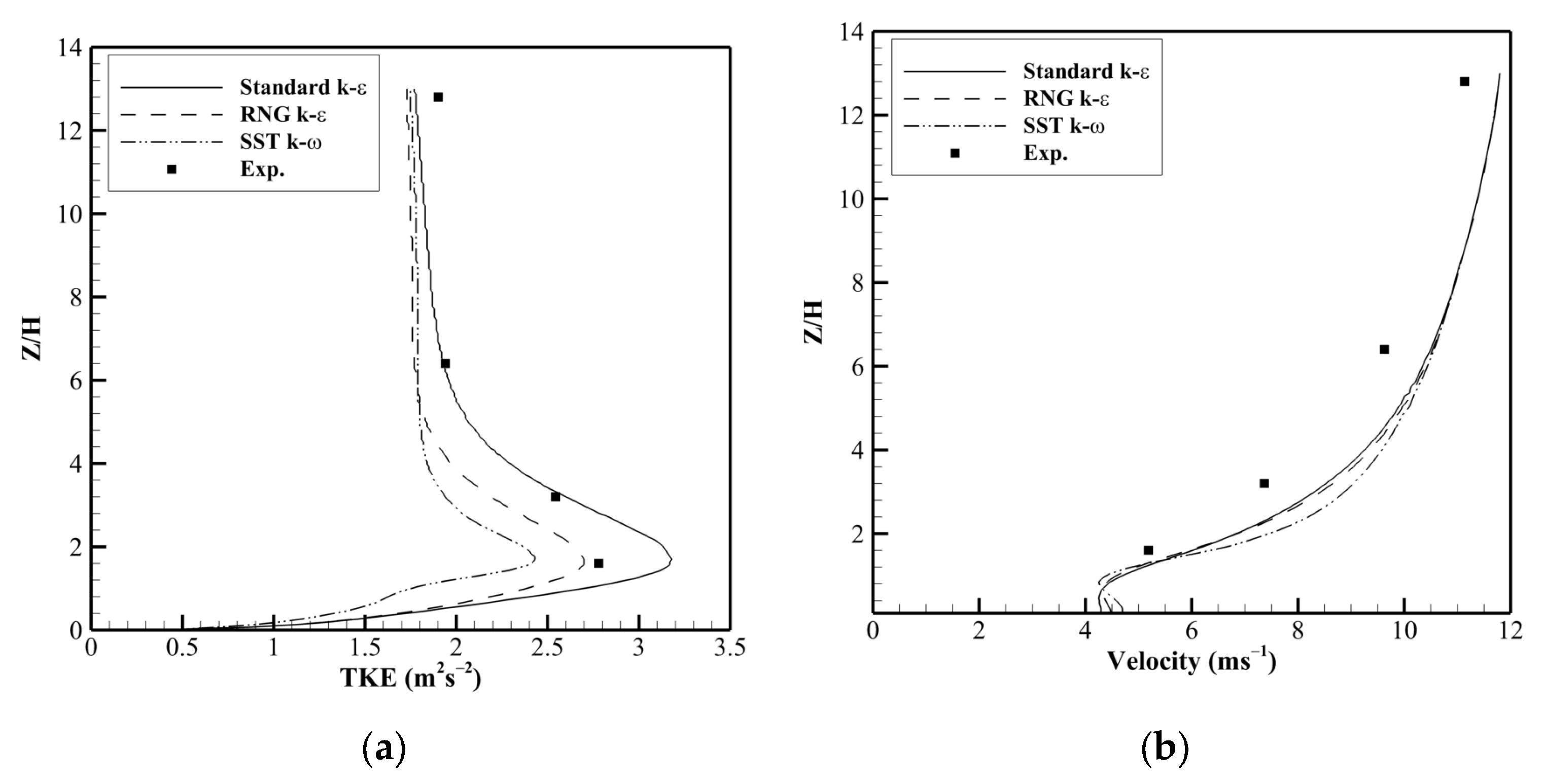
6.1. Performance Evaluation of Closure Models: Source Location Effects

The predicted turbulence field, especially the turbulence viscosity ( μ t ), has an undeniable impact on the accuracy of the predicted concentration field [64]. In addition to the expected differences due to the various definitions of μ t offered by each closure model, the produced turbulence by the available row of containers upstream of the source point also affects the predictions [65]. Using the appropriate computational grids, the performance of the selected turbulence models in predicting the concentration field was evaluated and compared in four cases with different types of the source location. Figure 3 illustrates the predicted concentration fields in all four trials represented by all three selected models, demonstrating clear distinctions in the vicinity of the source. However, as the pollutant plume progresses downstream, the differences in the predicted concentration fields at the plume centerline seem to be gradually reduced. Furthermore, it is evident from Figure 3 that the modeled concentration field by SST k ω promotes greater lateral spread of the plume compared to other models, with standard k ε showing the least.
Table 3 presents the calculated statistical measures for the point-to-point comparison in all the four selected trials. As can be seen, the statistical measures (except for VG) show values within the acceptable ranges, indicating the validity and reliability of the CFD results despite the selected closure models. The VG represents the unsystematic scatter of the predictions and is calculated to be larger than the acceptable limit for all cases. That refers to a relatively larger scatter that is primarily due to the available deviations at the edge of the plume, where the concentrations are relatively low, and even minor differences between observed and predicted values could lead to considerably large VG values.
The simulation results for Trial 1, where the scalar source is positioned midway between containers K8 and L8, show an overestimation of the concentration field in all cases (negative values of the FB). The net overprediction of the simulation results is further emphasized by the calculated MG values of less than 1, using all the three turbulence models. However, the overall superiority standard k ε closure is evident, with 62% of predicted concentrations within the FAC2 of the observed values. Further analysis of the parameters presented in Table 3 also suggests a relatively higher quality of the simulation results produced by standard k ε , showing less scatter (both linear, NMSE, and logarithmic, VG) compared with the field measurements.
As suggested by previous studies, the inaccurate representation of the turbulence field by two-equation viscosity models can be one of the primary sources of discrepancies found between the predictions and measurements [30,31,33]. In this regard, making a comparison between the predicted wind and turbulence flow field by all the studied closure models in this work is beneficial. Figure 4 maps the distribution of the turbulent kinetic energy (TKE) in the vicinity of the source location for Trial 1. Relatively higher TKE productions by standard k ε are observed near the source location, with the least values obtained by SST k ω model. The higher TKE values produced by standard k ε model further compliments the generated TKE by available containers in the geometry, which contradicts the well-established limitation of the RANS methods in underestimating the TKE fields [65]. Consequently, higher values of turbulence viscosity will be estimated by the standard k ε model that promotes higher particle diffusivity (assuming a constant S c t ), which justifies the relatively milder overprediction of the concentration field.
The estimated vertical profiles of the TKE and wind velocity obtained by the selected closure models at the central measuring tower are shown in Figure 5, along with the corresponding field measurements. As Figure 5a suggests, the standard k ε offers a more accurate representation of the TKE vertical variation compared to the two other closure models, with SST k ω predictions showing the largest deviations with the field data. Furthermore, the standard k ε model slightly overpredicts the TKE at the lower region of the ABL (where the available structures heavily affect the flow field), while the opposite is true in cases with the RNG k ε and SST k ω models. In addition, Figure 5b illustrates an overprediction of the velocity profile in all cases, with standard k ε outperforming the other closures. It should also be noted that the predicted velocity profiles are not considerably affected by the selection of the turbulence model, with a maximum relative difference of less than 7.2%.
The tracer gas in Trial 2 is released from a type A location, positioned immediately (1 m) upstream of the container J3. As shown in Table 3, 70% of the estimated concentrations using standard k ε are within a FAC2 of the observations, while this number is 65% and 64% for RNG k ε and SST k ω , respectively. Similar to Trial 1, negative values of the calculated linear fractional bias suggest that overpredicted concentration fields (near the plume centerline where the concentrations are high) were obtained by all the selected closure models. However, MG values larger than one indicate net underprediction in all cases, which is a consequence of underestimation of the concentrations near the edge of the plume. Considering the logarithmic nature of the MG, even minor discrepancies between the numerical results and measurements at the plume edge contribute to the determination of the net over/underprediction. Nonetheless, considering all the calculated statistical measures, the superiority of the results produced by the standard k ε model is evident.
The correct reproduction of the wind and turbulence field in the vicinity of the container J3 windward face is vital in capturing the initial spread of the scalar plume, which has a profound impact on the accuracy of the predicted concentration field. In this regard, the distributions of the TKE isolines in the vicinity of the scalar source are given in Figure 6. As it can be seen, larger values of TKE have been predicted using the standard k ε model near the source that is more than 0.3   m 2 s 2 , compared to less than 0.3   m 2 s 2 and 0.2   m 2 s 2 predicted by RNG k ε and SST k ω , respectively. The larger values of TKE, regardless of their accuracy concerning the field data, promote a greater particle diffusivity that results in predicting lower concentrations downstream. This explains the larger values of FB and MG for predictions made using the standard k ε (Table 3).
The estimated vertical profiles of TKE and wind velocity at the central tower inside the array are presented in Figure 7. As expected, both the k ε based models predicted larger values of TKE within the lower heights of the ABL, where the flow field is heavily affected by the presence of containers. However, by further progress in the z direction and moving away from the solid surfaces (ground and containers), the SST k ω gradually switches from the standard k ω to the standard k ε closure. As a result, larger values of TKE are estimated by SST k ω compared to RNG k ε from around an elevation of z / H = 5 aloft. All the turbulence models underpredict the TKE at the central tower, with the standard k ε showing a better agreement, which agrees with the presented statistical measures in Table 3. The estimated velocity profiles obtained by all three simulations of Trial 2 show minor differences with respect to each other and generally agree well with the field measurement at lower elevations. However, considerable deviations are observed from field data at the upper levels of the ABL, which could originate from the logarithmic profiles estimated at the inlet boundary [60]. Considering the height of the containers, z / H = 1 , these recorded discrepancies with actual wind velocities at higher elevations do not impact the accuracy of the predicted concentration fields.
Rooftop-based sources of air pollution (e.g., rooftop exhausts) are known as one of the main causes of air quality deterioration in compact urban regions. In this regard, Trial 3 has been purposely selected in this work for further evaluation of the modeling settings and methods. The scalar source in Trial 3 is of type D, positioned 10   cm above the container J9 roof. The standard k ε model significantly outperforms the other selected models by predicting 68% of the concentration field within the FAC2 of the field measurements. On the contrary, the SST k ω barely passes the validation assessment by only estimating 53% of the concentration field within the FAC2 of the field data. An overall overprediction of the scalar concentration field is observed, with calculated MG values of less than one and negative FB in all cases. Regarding the quality of results, the presented statistical measures in Table 3 strongly suggest the superiority of the standard k ε model, showing milder overall overpredictions (FB = 0.02 ) and relatively less scatter with the experiment (NMSE = 0.59 and VG = 3.13 ).
Figure 8 illustrates the estimated distributions of the TKE by all three turbulence models in the vicinity of the roof-based source. Consistent with previous studies [65,66], an overprediction of the TKE by the standard k ε is evident near the upwind corner of containers, leading to poor estimation of the separation flow. The TKE obtained by the standard k ε near the source is approximately 1.75   m 2 s 2 , compared to less than 1.0   m 2 s 2 and 0.75   m 2 s 2 predicted by RNG k ε and SST k ω , respectively. However, as previously mentioned, this overprediction of TKE makes up for the general underprediction of TKE by the RANS method [67], resulting in a more accurate representation of the concentration field downstream.
The vertical profiles of wind velocity and TKE at the central tower within the MUST array are presented in Figure 9. As shown in Figure 9a, all three closure models overpredict the TKE up to an elevation of z / H = 2 , with SST k ω performing relatively better. Furthermore, the deviation between numerical results and field measurements reduces with the elevation increase in ABL, where the effects of the available structures are negligible. Similar to what was discussed in two previous cases (Trials 1 and 2), the standard k−ε model produces higher levels of TKE, and as expected, its solution asymptotically approaches ones of SST k ω at higher elevations. Additionally, the wind velocity profiles estimated by all the three closures, Figure 9b, show a good agreement with the MUST measurements at lower heights, with k ε based closures performing slightly better.
The numerical modeling of Trial 4 provides the opportunity to evaluate the turbulence models if the source is located upstream outside of the array. As the statistical metrics in Table 3 indicate, all three closures performed relatively similarly when the scalar source and its initial spread were not impacted by the presence of obstacles (containers). This observation further justifies investigating the effects of the source location on the accuracy of predictions made by two-equation viscosity models. Both k ε based models predicted 65% of the resulted concentration field within a FAC2 of the MUST data, while the number is 61% for SST k ω . Furthermore, an overall minor tendency to underpredict the concentrations was observed using the standard k ε (with a FB of 0.07 and a MG of 1.01). RNG k ε and SST k ω , however, produced an overpredicted solution of the concentration field with an MG of 0.86 and 0.78, respectively. Assessing all five-performance metrics together, the overall superiority of the standard k ε is clear over the other two models, as all the calculated measures are within a closer range to the ideal values.
The distributions of the TKE isolines near the source, shown in Figure 10, further enforce the arguments made based on the statistical measures. As it can be seen, the predicted TKE fields by the three closure models are very similar in the vicinity of the scalar source. Taking a closer look at Figure 3, it can be clearly observed that all three representations of the concentration contours have similar shapes upstream of the array, and differences emerge as the generated plume passes the first row of containers. Therefore, having the source in regions where the simulated turbulence field is minimally affected by the type of the turbulence model (e.g., flow over an empty flat terrain) [41] seems to be an influencing factor in observing less distinction among the statistical measures presented for selected models.
Figure 11 plots the vertical velocity and TKE profiles at the central measuring tower of MUST geometry in Trial 4. Considerable underestimations of TKE at lower elevations are observed when SST k ω is used, which explains its less accurate representation of the concentration field (FAC2 of 61%). Using the standard k ε model, an overprediction of the TKE field is observed at lower heights, where the produced turbulence by available containers is available and compliments the TKE overprediction of this model. As the building-generated turbulence disappears after further progress aloft in the ABL, the reported TKE underprediction of RANS prevails, which consequently results in a general underestimation in all cases.
To further assess the accuracy of the CFD models, the predicted results in horizontal and vertical directions were also evaluated, and the calculated statistical measures are presented in Table 4. As the given performance metrics suggest, all three closure models offer a more accurate representation of the vertical concentration field than the horizontal field, with the standard k−ε model outperforming the other two closure models in every case. Additionally, less scatter is observed in vertical lines (lower VG values) than in all the horizontal sampling lines. The negative values of FB for vertical and the two immediate horizontal lines (sampling lines 1 and 2) indicate an overall over-prediction. In contrast, the opposite is valid for the two farther horizontal sampling lines where all three models generally under-predict the scalar concentration field.
The under-prediction of the scalar concentration on sampling Line 4 is much higher than the other lines, with FB values outside the acceptable range. It is suggested by Hanna et al. [68] that linear performance measures (FB and NMSE) could be excessively affected by randomly available large observed or modeled concentrations, which necessitates assessing the logarithmic metrics (MG and VG) to process them in a more balanced manner. A further look at the logarithmic measures also indicates excessive under-predictions (MG values larger than 1.3) and considerable scatter (VG values larger than 4.5) at the horizontal receptors of Line 4. Overall assessment of the statistical measures in Table 4 suggests that even though the accuracy and reliability of the predictions using standard k ε degrade as the distance from the source increases, this model performs considerably better than the other two on every level.
Scatter diagrams are presented for the horizontal and vertical sampling lines to better visualize the results of the conducted statistical analysis and the overall performance of the closure models in predicting the concentration field (Figure 12). The superiority of the standard k ε over the other two closure models is evident, predicting around 62% and 68% of the horizontal and vertical concentration fields within a FAC2 of the measurements, respectively. Aligned with the presented statistics in Table 4, the least scatter is observed for predictions made using the standard k ε , while the results obtained by SST k ω show the most. The predicted concentrations with relatively high values, which belong to the samplers near the source (e.g., sampling line 1) and along the plume centerline, are shown to be closer to the 1:1 line. In contrast, the predicted lower concentrations, mostly far from the source and the plume centerline, show considerably more scatter (this statement is supported by the performance measures provided in Table 4). Constantly varying meteorological conditions during field measurements, and inaccurate estimation of the inflow velocity and turbulence profiles, could be two possible reasons for this scatter.
In this regard, the effects of the inlet boundary conditions on the accuracy of the predicted results were first investigated by examining the wind direction in Trial 2. As mentioned before, the provided quantities in Table 1 are, in fact, the calculated mean values over the 200-s quasi-steady period. Regardless of how minor the variations in meteorological conditions are during the quasi-steady period, that could give rise to the well-known shortcomings of the RANS method. Knowing the standard deviation of 7.9 ° in the instantaneous inflow wind direction in Trial 2 [56], two more cases were simulated with different inflow wind directions of 22.1 ° and 37.9 ° . Considering the superiority of the standard k ε , this model was used as the closure to the RANS equations. Figure 13a shows the substantial deviation in the predicted concentration field caused by minor variations in the inflow wind direction during the field measurements, which further emphasizes the presence of discrepancies that could not be avoided.
The estimated inflow turbulence profiles are another known source of error in urban wind modeling. Figure 13b compares the predictions resulting from the estimated turbulence profiles, Equations (8) and (9), and the fitted inflow profiles using the available upstream measurements. As can be seen, a better agreement between predictions and observations is achieved by using the fitted turbulence profile at the inlet boundary instead of using the equilibrium equations. Noting that the detailed upstream measurements for every meteorological condition are scarce in actual applications, the estimated inflow profiles used in this study are shown to provide acceptable predictions.

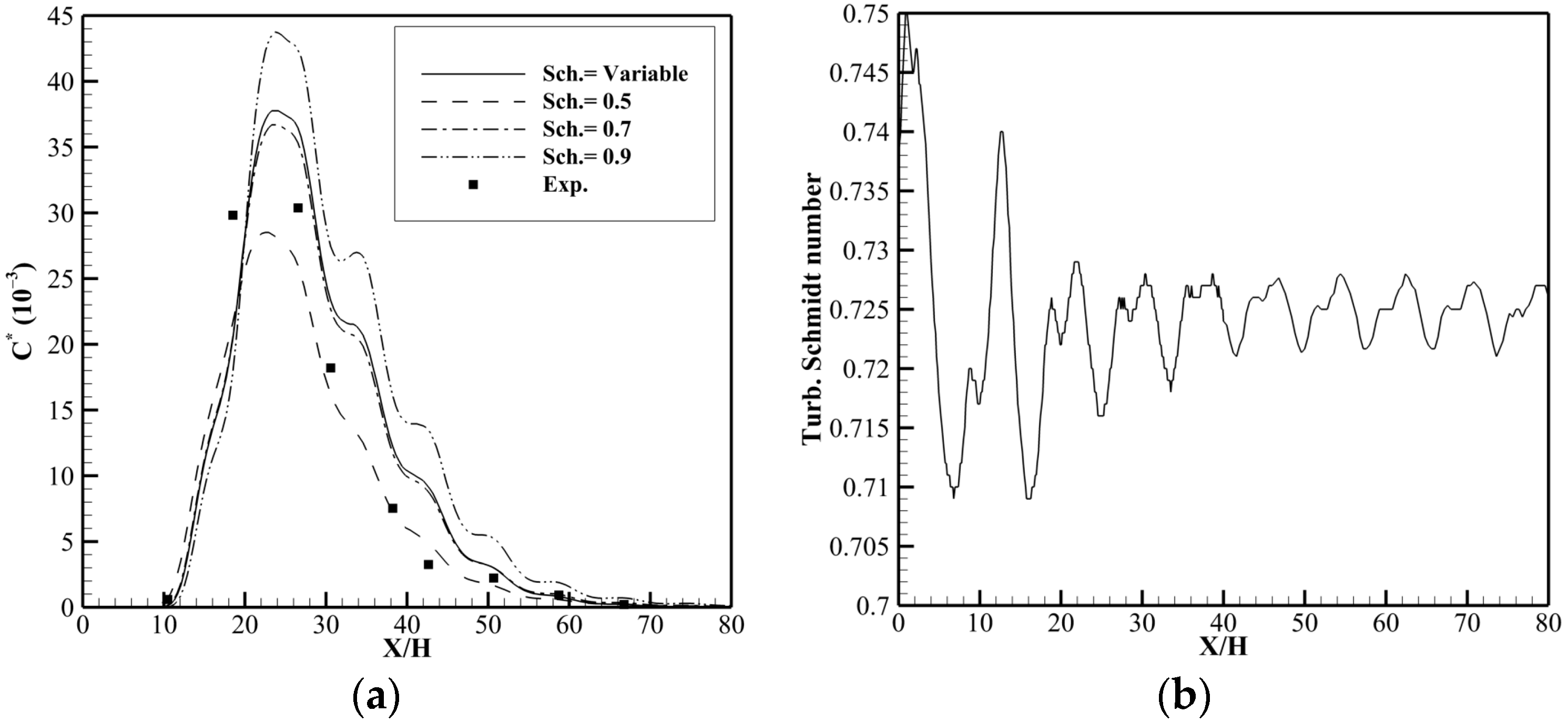
6.2. Turbulent Schmidt Number

The turbulent Schmidt number ( S c t ) is the next modeling parameter shown to considerably affect the predicted concentration field. Noting that there is no clear instruction on specifying the optimum S c t , different values are usually tested beforehand based on the physical characteristics of the geometry (e.g., natural landscapes, an isolated building, cluster of buildings, etc.) and the modeling scheme (e.g., turbulence closure model). Many studies have used different values of S c t specific to their cases, as a remedy to make up for the under/over-prediction of the turbulent diffusion [6,42,43,44]. The findings of a wind tunnel investigation by Koeltzsch, however, demonstrated the variation of the observed S c t with respect to the position in the boundary layer [69]. Additionally, several other studies strongly advised on the local variability of S c t [42,70]. Therefore, conducting pre-studies in generic cases is crucial to define S c t properly, as well as to evaluate the level of uncertainties associated with predictions.
Here, in addition to the conventional method of finding the optimum and constant value of S c t , the method of using a variable S c t will also be tested in the context of the dispersion modeling within complex urban geometries. For this purpose, Equation (18) will be incorporated into Equation (5) to account for the local variability of the S c t . Equation (18) was recently proposed by Longo et al. [71] with the purpose of estimating the optimum S c t based on the local turbulence state, which has shown promising results compared to very few other available S c t formulations [70]. S c in Equation (18) is the molecular Schmidt number, R e t is the turbulent Reynolds number, S is the strain-rate invariant, and Ω is the vorticity invariant.
S c t = e x p 0.6617 S c 0.8188 R e t 0.01 0.00311 S 0.0329 Ω
R e t = ρ k ω μ
S = k ε 2 S i j S i j                     S i j = 1 2 u ¯ i x j + u ¯ j x i
Ω = k ε 2 Ω i j Ω i j                   Ω i j = 1 2 u ¯ i x j u ¯ j x i
As an example, the results of further investigations done on Trial 3 (with a roof-based scalar source) to specify the optimum S c t are presented in this paper. Keeping in mind the superiority of the standard k ε in predicting the concentration fields, this closure model will be considered for the remaining studies of this research. Figure 14a shows the concentration profiles resulting from different S c t values at the first sampling line. The corresponding variable S c t , calculated using Equation (18), is also represented by Figure 14b. As Figure 14a shows, increasing the S c t will generally result in larger values of C * to be predicted by the numerical model. This clearly shows the inverse relation of the turbulent diffusivity with S c t , which provides the modeler with the opportunity to control over/underpredictions of scalar diffusion. An initial analysis of Figure 14a also indicates that S c t = 0.5 provides relatively better predictions of the concentration field, except at the plume centerline, where it considerably underpredicts the peak values. Accurate prediction of relatively higher pollutant concentrations near the plume centerline is of great importance due to exposure-related complications that might arise. Therefore, to better evaluate the results of this sensitivity study, a detailed statistical analysis was conducted on the predicted concentration field for a wide range of S c t .
The numerical results obtained using S c t of 0.3, 1.1, and 1.3 are shown to have inadequate qualities to be considered for further investigations in this work. It also can be concluded from Table 5 that even though S c t = 0.5 results in FAC2 of 0.76, it generally provides predictions with an unacceptable level of underprediction (FB = 0.42). The relatively large value of the MG (1.22) further indicates the net underprediction of the concentration field obtained using S c t of 0.5. Considering all the performance metrics provided in Table 5, a constant S c t of 0.7 appears to be the optimum value in this case study while showing relatively milder underpredictions (FB of 0.16 and MG of 0.97) and fewer linear and logarithmic scatters (NMSE of 0.40 and VG of 1.74). It is noteworthy that implementing the variable S c t , Equation (18), instead of using the conventional “constant value” approach, also resulted in performance metrics quite similar to the optimum S c t (0.7). Figure 14b maps the variation of the predicted S c t by Equation (18) in the selected case study, which shows its fluctuations between 0.7 and 0.75. This justifies the implementation of this method in future applications and studies that lack field measurements for carrying out a validation study to determine the optimum S c t .

7. Conclusions

A sensitivity study was carried out to evaluate the performance of the most widely used two-equation turbulence models to form a well-tested framework for representing the pollutant dispersion flow within a compact urban geometry. Four distinct case studies of the MUST comprehensive dispersion dataset were chosen to further investigate the impacts of the source location on the accuracy of the concentration fields predicted by the closure models. The sources in Trials 1–3 are located within the MUST array, where the structure-generated turbulence substantially influences the plume’s immediate spread. The source in Trial 4, however, is positioned upstream and outside of the array, where all three closure models estimate similar representations of the turbulence fields (flow over an open flat terrain). Somewhat similar performance measures (FAC2 of 65% for k ε based models and 61% for SST k ω model) were calculated for predictions obtained by all closure models in Trial 4 compared to other case studies, which further justified the importance of conducting this sensitivity study.
Overall, Standard k ε showed superiority in predicting the concentration fields for all the selected trials, with higher calculated FAC2 than the other two models. Except for Trial 4, the negative value of the calculated linear fractional biases (FB) indicated overprediction by the CFD models, in which the standard k ε showed better performance compared to the two other closure models. In comparison to Trials 1–3, the predictions in Trial 4 obtained by the Standard k ε showed minimal underprediction (positive values of FB). RANS methods are known for underestimating the TKE field due to their inability to reproduce the large-scale eddies, which generally results in underestimating the turbulent diffusivity and, consequently, overpredicting the concentration field. However, the turbulence produced by the available obstacles (here, containers) in compact urban geometries will make up for the underestimation of the TKE by RANS models. The buildings’ effects on turbulence, combined with the reported overestimation of the TKE by Standard k ε , leads to milder overprediction of the concentration field by this closure model in Trials 1–3. Similar reasoning also justifies the relatively higher positive FB value (0.07) calculated by the standard k ε model in Trial 4.
To further improve the accuracy of the simulations, another sensitivity study was also carried out to determine the proper value of the S c t . Following the conventional procedure in finding the optimum S c t , several values in the range of 0.3–1.3 were tested, and the resultant concentration fields were compared with the field measurements. An optimum S c t of around 0.7 was found to produce the most accurate and reliable results. However, acquiring a high-quality dispersion dataset for most applications in actual geometries is quite challenging and impractical to do in similar sensitivity studies. In this regard, another approach was tested in the context of a compact urban geometry, in which the S c t was defined as a locally variable parameter. The calculated S c t varied in the range of 0.7–0.75, and considerable improvements were observed in the accuracy of the predictions.

Author Contributions

Conceptualization, M.R.K.N., B.A.F. and C.F.L.; methodology, M.R.K.N., B.A.F. and C.F.L.; software, M.R.K.N.; validation, M.R.K.N.; formal analysis, M.R.K.N.; investigation, M.R.K.N.; resources, B.A.F.; data curation, M.R.K.N.; writing—original draft preparation, M.R.K.N.; writing—review and editing, M.R.K.N., B.A.F. and C.F.L.; visualization, M.R.K.N.; supervision, B.A.F. and C.F.L.; project administration, B.A.F.; funding acquisition, B.A.F. All authors have read and agreed to the published version of the manuscript.

Funding

This research was funded by the Natural Sciences and Engineering Council of Canada (NSERC) with the Discovery Grant number RGPIN-2020-03896 from B. Fleck.

Institutional Review Board Statement

Not applicable.

Informed Consent Statement

Not applicable.

Data Availability Statement

Not applicable.

Acknowledgments

The authors would like to thank the Defense Threat Reduction Agency (DTRA) for providing access to the MUST dispersion dataset.

Conflicts of Interest

The authors declare no conflict of interest.

References

  1. 2018 Revision of World Urbanization Prospects, Technical Report; United Nations Department of Economics and Social Affairs (UNDESA): New York, NY, USA, 2018.
  2. Wilson, D.J.; Britter, R.E. Estimates of building surface concentrations from nearby point sources. Atmos. Environ. 1982, 16, 2631–2646. [Google Scholar] [CrossRef]
  3. ASHRAE. Airflow around the buildings. In ASHRAE Fundamental Handbook; American Society of Heating, Refrigerating and Air-conditioning Engineers: Atlanta, GA, USA, 2009. [Google Scholar]
  4. Hajra, B.; Stathopoulos, T.; Bahloul, A. Assessment of pollutant dispersion from rooftop stacks: ASHRAE, ADMS and wind tunnel simulation. Build. Environ. 2010, 45, 2768–2777. [Google Scholar] [CrossRef]
  5. Holmes, N.S.; Morawska, L. A review of dispersion modeling and its application to the dispersion of particles: An overview of different dispersion models available. Atmos. Environ. 2006, 40, 5902–5928. [Google Scholar] [CrossRef] [Green Version]
  6. Riddle, A.; Carruthers, D.; Sharpe, A.; McHugh, C.; Stocker, J. Comparisons between FLUENT and ADMS for atmospheric dispersion modeling. Atmos. Environ. 2004, 38, 1029–1038. [Google Scholar] [CrossRef]
  7. Lateb, M.; Masson, C.; Stathopoulos, T.; Bedard, C. Effect of stack height and exhaust velocity on pollutant dispersion in the wake of a building. Atmos. Environ. 2011, 45, 5150–5163. [Google Scholar] [CrossRef] [Green Version]
  8. Li, Z.; Ming, T.; Liu, S.; Peng, C.; Richter, R.; Li, W.; Zhang, H.; Wen, C.Y. Review on pollutant dispersion in urban areas-part A: Effects of mechanical factors and urban morphology. Build. Environ. 2021, 190, 107534. [Google Scholar] [CrossRef]
  9. Du, Y.; Blocken, B.; Abbasi, S.; Pirker, S. Efficient and high-resolution simulation of pollutant dispersion in complex urban environments by island-based recurrence CFD. Environ. Model. Softw. 2021, 145, 105172. [Google Scholar] [CrossRef]
  10. Ricci, A.; Kalkman, I.; Blocken, B.; Burlando, M.; Freda, A.; Repetto, M. Local-scale forcing effects on wind flows in an urban environment: Impact of geometrical simplifications. J. Wind. Eng. Ind. Aerodyn. 2017, 170, 238–255. [Google Scholar] [CrossRef]
  11. Lee, D.S.H.; Mauree, D. RANS based CFD simulations for urban wind prediction–field verification against MoTUS. Wind. Struct. 2021, 33, 29–40. [Google Scholar]
  12. Silva, F.T.; Reis, N.C.; Santos, J.M.; Goulart, E.V.; Alvarez, C.E. The impact of urban block typology on pollutant dispersion. J. Wind. Eng. Ind. Aerodyn. 2021, 210, 104524. [Google Scholar] [CrossRef]
  13. Mattar, S.J.; Kavian Nezhad, M.R.; Versteege, M.; Lange, C.F.; Fleck, B.A. Validation Process for Rooftop Wind Regime CFD Model in Complex Urban Environment Using an Experimental Measurement Campaign. Energies 2021, 14, 2497. [Google Scholar] [CrossRef]
  14. Wilson, D.J.; Lamb, B.K. Dispersion of exhaust gases from roof-level stacks and vents on a laboratory building. Atmos. Environ. 1994, 28, 3099–3111. [Google Scholar] [CrossRef]
  15. Yang, C.; Hong, Z.; Chen, j.; Xu, L.; Zhuang, M.; Huang, Z. Characteristics of secondary organic aerosols tracers in PM2.5 in three central cities of the Yangtze river delta, China. Chemosphere 2022, 293, 133637. [Google Scholar] [CrossRef]
  16. Dai, Y.; Mak, C.M.; Hang, J.; Zhang, F.; Ling, H. Scaled outdoor experimental analysis of ventilation and interunit dispersion with wind and buoyancy effects in street canyons. Energy Build. 2022, 255, 111688. [Google Scholar] [CrossRef]
  17. Lateb, M.; Meroney, R.N.; Yataghene, M.; Fellouah, H.; Saleh, F.; Boufadel, B.C. On the use of numerical modeling for near-field pollutant dispersion in urban environment. Environ. Pollut. 2016, 208, 271–283. [Google Scholar] [CrossRef] [Green Version]
  18. Hajra, B.; Stathopoulos, T.; Bahloul, A. A wind tunnel study of the effects of adjacent buildings on near-field pollutant dispersion from rooftop emissions in an urban environment. J. Wind. Eng. Ind. Aerodyn. 2013, 119, 133–145. [Google Scholar] [CrossRef]
  19. Zou, J.; Yu, Y.; Liu, J.; Niu, J.; Chauhan, K.; Lei, C. Field measurement of the urban pedestrian level wind turbulence. Build. Environ. 2021, 194, 107713. [Google Scholar] [CrossRef]
  20. Lateb, M.; Masson, C.; Stathopoulos, T.; Bedard, C. Numerical simulation of pollutant dispersion around a building complex. Build. Environ. 2010, 45, 1788–1798. [Google Scholar] [CrossRef] [Green Version]
  21. Mirzaei, P.A. CFD modeling of micro and urban climates: Problems to be solved in the new decade. Sustain. Cities Soc. 2021, 69, 102839. [Google Scholar] [CrossRef]
  22. Du, Y.; Blocken, B.; Pirkar, S. A novel approach to simulate pollutant dispersion in the built environment: Transport-based recurrence CFD. Build. Environ. 2020, 170, 106604. [Google Scholar] [CrossRef]
  23. Jiang, G.; Yoshie, R. Side ratio effects on flow and pollutant dispersion around an isolated high-rise building in a turbulent boundary layer. Build. Environ. 2020, 180, 107078. [Google Scholar] [CrossRef]
  24. Huang, X.; Gao, L.; Guo, D.; Yao, R. Impacts of high-rise building on urban airflows and pollutant dispersion under different temperature stratifications: Numerical investigations. Atmos. Pollut. Res. 2021, 12, 100–112. [Google Scholar] [CrossRef]
  25. Chavez, M.; Hajra, B.; Stathopoulos, T.; Bahloul, A. Assessment of near-field pollutant dispersion: Effect of upstream buildings. J. Wind. Eng. Ind. Aerodyn. 2012, 104, 509–515. [Google Scholar] [CrossRef]
  26. Lauriks, T.; Longo, R.; Baetens, D.; Derudi, M.; Parente, A.; Bellemans, A.; Van Beeck, J.; Denys, S. Application of improved CFD modeling for prediction and mitigation of traffic related air pollution hotspots in a realistic urban street. Atmos. Environ. 2021, 246, 118127. [Google Scholar] [CrossRef]
  27. Salim, S.M.; Buccolieri, R.; Chan, A.; Sabatino, S.D. Numerical simulation of atmospheric pollutant dispersion in an urban street canyon: Comparison between RANS and LES. J. Wind. Eng. Ind. Aerodyn. 2011, 99, 103–113. [Google Scholar] [CrossRef]
  28. Zheng, X.; Yang, J. CFD simulation of wind flow and pollutant dispersion in a street canyon with traffic flow: Comparison between RANS and LES. Sustain. Cities Soc. 2021, 75, 103307. [Google Scholar] [CrossRef]
  29. Versteeg, H.K.; Malalasekera, W. Introduction to Computational Fluid Dynamics, 2nd ed.; Pearson Education Limited: Harlow, UK, 2007. [Google Scholar]
  30. Narjisse, A.; Abdellatif, K. Assessment of RANS turbulence closure models for predicting airflow in neutral ABL over hilly terrain. Int. Rev. Apllied Sci. Eng. 2021, 12, 238–256. [Google Scholar] [CrossRef]
  31. Tominaga, Y. Flow around a high-rise building using steady and unsteady RANS CFD; Effect of large-scale fluctuations on the velocity statics. J. Wind. Eng. Ind. Aerodyn. 2015, 142, 93–103. [Google Scholar] [CrossRef]
  32. Hosseinzadeh, A.; Keshmiri, A. Computational simulation of wind microclimate in complex urban models and mitigation using tress. Buildings 2021, 11, 112. [Google Scholar] [CrossRef]
  33. Lateb, M.; Masson, C.; Stathopoulos, T.; Bedard, C. Comparison of various types of k–e models for pollutant emissions around a two-building configuration. J. Wind. Eng. Ind. Aerodyn. 2013, 115, 9–21. [Google Scholar] [CrossRef] [Green Version]
  34. An, K.; Fung, J.C.H. An improved SST k-w model for pollutant dispersion simulations within an isothermal boundary layer. J. Wind. Eng. Ind. Aerodyn. 2018, 179, 369–384. [Google Scholar] [CrossRef]
  35. Keshavarzian, E.; Jin, R.; Dong, K.; Kwok, K.C.S.; Zhang, Y.; Zhao, M. Effect of pollutant source location on air pollutant dispersion around a high-rise building. Appl. Math. Modeling 2020, 81, 582–602. [Google Scholar] [CrossRef] [PubMed]
  36. Hassan, A.M.; ELMokadem, A.A.; Megahed, N.A.; Abo Eleinen, O.M. Urban morphology as a passive strategy in promoting outdoor air quality. J. Build. Eng. 2020, 29, 101204. [Google Scholar] [CrossRef]
  37. Ming, T.; Shi, T.; Han, H.; Liu, S.; Wu, Y.; Li, W. Assessment of pollutant dispersion in urban street canyons based on field synergy theory. Atmos. Pollut. Res. 2021, 12, 341–356. [Google Scholar] [CrossRef]
  38. Pirhalla, M.; Heist, D.; Perry, S.; Tang, W.; Brouwer, L. Simulations of dispersion through an irregular urban building array Michael. Atmos. Environ. 2021, 258, 118500. [Google Scholar] [CrossRef]
  39. Elfverson, D.; Lejon, C. Use and scalability of OpenFOAM for wind fields and pollution dispersion with building- and ground-resolving topography. Atmosphere 2021, 12, 1124. [Google Scholar] [CrossRef]
  40. Blocken, B. LES over RANS in building simulation for outdoor and indoor applications: A foregone conclusion? Build. Simul. 2018, 11, 821–870. [Google Scholar] [CrossRef] [Green Version]
  41. Blocken, B.; Stathopoulos, T.; Carmeliet, J. CFD simulation of the atmospheric boundary layer: Wall function problems. Atmos. Environ. 2007, 41, 238–252. [Google Scholar] [CrossRef]
  42. Tominaga, Y.; Stathopoulos, T. Turbulent Schmidt numbers for CFD analysis with various types of flowfield. Atmos. Environ. 2007, 41, 8091–8099. [Google Scholar] [CrossRef]
  43. Di Sabatino, S.; Buccolieri, R.; Pulvirenti, B.; Britter, R. Simulations of pollutant dispersion within idealised urban-type geometries with cfd and integral models. Atmos. Environ. 2007, 41, 8316–8329. [Google Scholar] [CrossRef]
  44. Blocken, B.; Stathopoulos, T.; Saathoff, P.; Wang, X. Numerical evaluation of pollutant dispersion in the built environment: Comparisons between models and experiments. J. Wind. Eng. Ind. Aerodyn. 2008, 96, 1817–1831. [Google Scholar] [CrossRef] [Green Version]
  45. Emeis, S. Wind Energy Meteorology Atmospheric Physics for Wind Power Generation, 2nd ed.; Springer International Publishing AG: Zug, Switzerland, 2018; pp. 31–56. [Google Scholar]
  46. Speranza, A.; Lucarini, V. Environmental science, physical principles and applications. Encycl. Condens. Matter Phys. 2005, 146–156. [Google Scholar]
  47. Mohamed, M.A.; Wood, D.H. Computational modeling of wind flow over the University of Calgary campus. Wind. Eng. 2016, 40, 228–249. [Google Scholar] [CrossRef]
  48. Menter, F.R. Two-equation eddy-viscosity turbulence modes for engineering applications. AIAA J. 1994, 32, 1598–1605. [Google Scholar] [CrossRef] [Green Version]
  49. ANSYS, Inc. ANSYS CFX-Solver Theory Guide Release 2020-R1; ANSYS, Inc.: Canonsburg, PA, USA, 2020; pp. 79–90. [Google Scholar]
  50. Milliez, M.; Carissimo, B. Numerical simulations of pollutant dispersion in an idealized urban area, for different meteorological conditions. Bound. Layer Meteorol. 2007, 122, 321–342. [Google Scholar] [CrossRef]
  51. Donnelly, R.P.; Lyons, T.J.; Flassak, T. Evaluation of results of a numerical simulation of dispersion in an idealised urban area for emergency response modelling. Atmos. Environ. 2009, 43, 4416–4423. [Google Scholar] [CrossRef] [Green Version]
  52. Kumar, P.; Feiz, A.; Singh, S.K.; Ngae, P. An urban scale inverse modelling for retrieving unknown elevated emissions with building-resolving simulations. Atmos. Environ. 2016, 140, 135–146. [Google Scholar] [CrossRef] [Green Version]
  53. Bahlali, M.L.; Dupont, E.; Carissimo, B. Atmospheric dispersion using a Lagrangian stochastic approach: Application to an idealized urban area under neutral and stable meteorological conditions. J. Wind. Eng. Ind. Aerodyn. 2019, 193, 103976. [Google Scholar] [CrossRef]
  54. Tee, C.; Ng, E.Y.K.; Xu, G. Analysis of transport methodologies for pollutant dispersion modelling in urban environments. J. Environ. Chem. Eng. 2020, 8, 103937. [Google Scholar] [CrossRef]
  55. Biltoft, C.A. Customer Report for Mock Urban Setting Test; Technical Report, DPG Document No. WDTC-FR-01–121; US Army Dugway Proving Ground: Dugway, UT, USA, 2001. [Google Scholar]
  56. Yee, E.; Biltoft, C. Concentration fluctuation measurements in a plume dispersing through a regular array of obstacles. Bound. Layer Meteorol. 2004, 111, 363–415. [Google Scholar] [CrossRef]
  57. Zhang, Z.; Wang, K. Quantifying and adjusting the impact of urbanization on the observed surface wind speed over China from 1985 to 2017. Fundam. Res. 2021, 1, 785–791. [Google Scholar] [CrossRef]
  58. Franke, J.; Hellsten, A.; Schlünzen, H.; Carissimo, B. Best Practice Guideline for the CFD Simulation of Flows in the Urban Environment: COST Action 732 Quality Assurance and Improvement of Microscale Meteorological Models; Meteorological Inst.: Hamburg, Germany, 2007. [Google Scholar]
  59. Tian, L.; Zhao, N.; Wang, T.; Zhu, W.; Shen, W. Assessment of inflow boundary conditions for RANS simulations of neutral ABL and wind turbine wake flow. J. Wind. Eng. Ind. Aerodyn. 2018, 179, 215–228. [Google Scholar] [CrossRef]
  60. Richards, P.J.; Hoxey, R.P. Appropriate boundary conditions for computational wind engineering models using the k-ε turbulence model. J. Wind. Eng. Ind. Aerodyn. 1993, 46, 145–153. [Google Scholar] [CrossRef]
  61. Celik, I.B.; Ghia, U.; Roache, P.J.; Freitas, C.J.; Coleman, H.; Raad, P.E. Procedure for estimation and reporting of uncertainty due to discretization in CFD applications. J. Fluids Eng. 2008, 130, 078001. [Google Scholar] [CrossRef] [Green Version]
  62. Roache, P.J. Quantification of uncertainty in computational fluid dynamics. Annu. Rev. Fluid Mech. 1997, 29, 123–160. [Google Scholar] [CrossRef] [Green Version]
  63. Chang, J.C.; Hanna, S.R. Air quality model performance evaluation. Meteorol. Atmos. Phys. 2004, 87, 167–196. [Google Scholar] [CrossRef]
  64. Tominaga, Y.; Stathopoulos, T. Numerical simulation of dispersion around an isolated cubic building: Comparison of various types of k-e models. Atmos. Environ. 2009, 20, 3200–3210. [Google Scholar] [CrossRef]
  65. Tominaga, Y.; Stathopoulos, T. CFD simulation of near-field pollutant dispersion in the urban environment: A review of current modeling techniques. Atmos. Environ. 2013, 79, 716–730. [Google Scholar] [CrossRef] [Green Version]
  66. Murakami, S. Comparison of various turbulence models applied to a bluff body. J. Wind. Eng. Ind. Aerodyn. 1993, 46, 21–36. [Google Scholar] [CrossRef]
  67. Tominaga, Y.; Stathopoulos, T. Numerical simulation of dispersion around an isolated cubic building: Model evaluation of RANS and LES. Build. Environ. 2010, 45, 2231–2239. [Google Scholar] [CrossRef] [Green Version]
  68. Hanna, S.R.; Hansen, O.R.; Dharmavaram, S. FLACS CFD air quality model performance evaluation with Kit Fox, MUST, Prairie Grass, and EMU observations. Atmos. Environ. 2004, 38, 4675–4687. [Google Scholar] [CrossRef]
  69. Koeltzsch, K. The height dependence of the turbulent Schmidt number within the boundary layer. Atmos. Environ. 2000, 34, 1147–1151. [Google Scholar] [CrossRef]
  70. Longo, R.; Fürsta, M.; Bellemansa, A.; Ferrarottia, M.; Derudib, M.; Parentea, A. CFD dispersion study based on a variable Schmidt formulation for flows around different configurations of ground-mounted buildings. Build. Environ. 2019, 154, 336–347. [Google Scholar] [CrossRef] [Green Version]
  71. Longo, R.; Bellemansa, A.; Derudib, M.; Parentea, A. A multi-fidelity framework for the estimation of the turbulent Schmidt number in the simulation of atmospheric dispersion. Build. Environ. 2020, 185, 107066. [Google Scholar] [CrossRef]
Figure 1. (a) Planar schematic view of MUST container array; (b) Schematic view of all six types of releasing locations.
Atmosphere 13 01013 g001
Figure 2. Comparison of concentration profiles at the first horizontal sampling line in Trial 1 for (a) cases with SST k ω and for (b) cases with k ε based closure models.
Atmosphere 13 01013 g002
Figure 3. Contours of the predicted concentration field obtained by (a) Standard k ε , (b) RNG k ε , and (c) SST k ω models on a horizontal plane at z / H = 0.64 (The height at which all horizontal PIDs are installed).
Atmosphere 13 01013 g003aAtmosphere 13 01013 g003b
Figure 4. The turbulence kinetic energy, TKE m 2 s 2 , distribution in the vicinity of the source location (red circle) in Trial 1 obtained by (a) Standard k ε , (b) RNG k ε , and (c) SST k ω models.
Atmosphere 13 01013 g004
Figure 5. Comparison of vertical profiles of (a) TKE and (b) velocity at the 32 m central tower with the field measurements of Trial 1.
Atmosphere 13 01013 g005
Figure 6. The turbulence kinetic energy, TKE m 2 s 2 , distribution in the vicinity of the source location (red circle) in Trial 2 obtained by (a) Standard k ε , (b) RNG k ε , and (c) SST k ω models.
Atmosphere 13 01013 g006
Figure 7. Comparison of vertical profiles of (a) TKE and (b) velocity at the 32 m central tower with the field measurements of Trial 2.
Atmosphere 13 01013 g007
Figure 8. The turbulence kinetic energy, TKE m 2 s 2 , distribution in the vicinity of the source location (red circle) in Trial 3 obtained by (a) Standard k ε , (b) RNG k ε , and (c) SST k ω models.
Atmosphere 13 01013 g008aAtmosphere 13 01013 g008b
Figure 9. Comparison of vertical profiles of (a) TKE and (b) velocity at the 32 m central tower with the field measurements of Trial 3.
Atmosphere 13 01013 g009
Figure 10. The turbulence kinetic energy, TKE m 2 s 2 , distribution in the vicinity of the source location (red circle) in Trial 4 obtained by (a) Standard k ε , (b) RNG k ε , and (c) SST k ω models.
Atmosphere 13 01013 g010
Figure 11. Comparison of vertical profiles of (a) TKE and (b) velocity at the 32 m central tower with the field measurements of Trial 4.
Atmosphere 13 01013 g011
Figure 12. Scatter diagrams between the predicted and observed concentrations in (a) horizontal and (b) vertical sampling lines.
Atmosphere 13 01013 g012
Figure 13. Comparison of the C * profiles at the first horizontal sampling line in Trial 2 for different (a) inflow wind directions and (b) inflow turbulence profiles.
Atmosphere 13 01013 g013
Figure 14. (a) C * for different S c t , and (b) the corresponding variable S c t for the first sampling line of Trial 3.
Atmosphere 13 01013 g014
Table 1. Four selected trials of MUST field experiment.
Trial No.Trial I.D. q s   l m i n Source Type Z s   m S 04   m s α 04   d e g u τ   m / s L O   m k   m 2 / s 2
12681829225F1.87.93−411.1028,0001.46
22672213200A1.82.68300.351500.428
32682320225D2.64.55−390.501700.718
42692250225E1.33.38360.371300.537
Table 2. Results of the grid independence analysis.
Turbulence Closure Model Number   of   Computational   Nodes   ( 10 6 ) Coarse-MediumMedium-Fine
CoarseMediumFine e a % G C I % e a % G C I %
SST k ω 7.6511.5917.5014.0039.771.975.60
k ε based models6.399.6814.625.6115.942.336.62
Table 3. Statistical evaluation of the concentration predictions for the selected trials.
CaseModelFBNMSEVGMGFAC2
Trial 1Standard k ε −0.010.792.650.980.62
RNG k ε −0.171.453.110.840.59
SST k ω −0.232.063.810.800.59
Trial 2Standard k ε −0.111.042.351.240.70
RNG k ε −0.252.213.761.130.65
SST k ω −0.202.235.651.060.64
Trial 3Standard k ε −0.020.593.130.850.68
RNG k ε −0.220.763.250.940.58
SST k ω −0.290.665.360.970.53
Trial 4Standard k ε 0.070.461.981.010.65
RNG k ε 0.000.622.540.860.65
SST k ω 0.011.013.510.780.61
Table 4. Statistical evaluation of the concentration predictions at horizontal and vertical sampling lines.
Sampling lineModelFBNMSEVGMGFAC2
Line 1Standard k ε −0.181.361.860.910.67
RNG k ε −0.392.922.420.790.50
SST k ω −0.483.215.670.840.38
Line 2Standard k ε −0.040.562.880.830.58
RNG k ε −0.180.955.690.710.50
SST k ω −0.110.905.850.530.53
Line 3Standard k ε 0.250.883.860.860.64
RNG k ε 0.171.154.120.930.58
SST k ω 0.381.666.811.160.53
Line 4Standard k ε 0.591.564.551.390.56
RNG k ε 0.671.994.641.560.56
SST k ω 0.812.566.661.810.53
VerticalStandard k ε −0.081.491.740.990.68
RNG k ε −0.181.162.370.840.61
SST k ω −0.121.663.220.850.61
Table 5. Statistical evaluation of the C * predictions of Trial 3 for different S c t .
Turb. Schmidt NumberFBNMSEVGMGFAC2
0.30.861.484.572.400.50
0.50.420.441.971.220.76
0.70.160.401.740.970.71
0.9−0.020.593.130.850.68
1.1−0.150.857.790.790.62
1.3−0.231.1222.270.780.55
Variable0.130.411.820.980.71
Publisher’s Note: MDPI stays neutral with regard to jurisdictional claims in published maps and institutional affiliations.

