Article

Large-Eddy Simulation of Airflow and Pollutant Dispersion in a Model Street Canyon Intersection of Dhaka City

1
Department of Mathematics & Physics, North South University, Dhaka 1229, Bangladesh
2
Center for Applied and Scientific Computing (CASC), North South University, Dhaka 1229, Bangladesh
3
School of Civil Engineering, University of Leeds, Leeds LS2 9JT, UK
4
Agriculture Victoria Research, Department of Jobs, Precincts and Regions, Victoria State Government, Melbourne, VIC 3083, Australia
5
School of Computing, Engineering and Mathematical Sciences, La Trobe University, Melbourne, VIC 3086, Australia
*
Author to whom correspondence should be addressed.
Atmosphere 2022, 13(7), 1028; https://doi.org/10.3390/atmos13071028
Submission received: 2 June 2022 / Revised: 20 June 2022 / Accepted: 21 June 2022 / Published: 28 June 2022
(This article belongs to the Special Issue Computational Fluid Dynamics Simulations of Urban Airflow)

Abstract

:
The atmospheric flow and dispersion of traffic exhaust were numerically studied in this work while considering a model street canyon intersection of a city. The finite volume method (FVM)-based large-eddy simulation (LES) technique in line with ANSYS Fluent have been used for flow and pollutant dispersion modelling through the consideration of the atmospheric boundary layer (ABL). Hexahedral elements are considered for computational domain discretization in order to numerically solve problems using FVM-LES. The turbulence parameters were superimposed through a spectral synthesizer in the existing LES model through ANSYS Fluent as part of ’damage control’ due to the unsteady k ϵ simulation. Initially, the code is validated with an experimental study of an urban street canyon where the width and height ratio is in unity. After validation, a model urban street canyon intersection was investigated in this work. The model shows a high pollutant concentration in the intersecting corner areas of the buildings. Additionally, the study of this model intersection shows a high level of pollutant concentration at the leeward wall of downwind building in the case of increased height of an upwind building. Most importantly, it was realized from the street intersection design that three-dimensional interconnection between the dominating canyon vortices and roof level flow plays a pivotal role in pollutant concentration level on the windward walls. The three-dimensional extent of corner eddies and their interconnections with dominating vortices were found to be extremely important as they facilitate enhanced ventilation. Corner eddies only form for the streets towards the freeway and not for the streets towards the intersection. The results and key findings of this work offer qualitative and quantitative data for the estimation, planning, and implementation of exposure mitigation in an urban environment.

1. Introduction

The term “street canyon” simply refers to a type of narrow street between buildings lining up in continuous order in both sides, which mostly occurs in urban areas. Street canyons can exhibit a different climate from the nearby areas, specifically when the areas are heavily influenced by the micro-scale meteorological process [1,2]. Another challenge concerning street canyons is ventilation and pollutant dispersion, where the latter indicates the transportation of air pollutants through the outdoor atmosphere. In any case, both processes usually take place through the roof level in a street canyon [1,3,4]. Therefore, air quality near street canyons is often indexed as poor and that is why it is a major issue for the inhabitants. As a result, more studies are still required, particularly those targeting densely populated commercial areas. Dhaka is a major city and the capital of Bangladesh. The city, which is a particular area of interest of this study, because it often faces severe air quality problems near the street canyons not only from rooftop pollutant dispersion, but also from heavy traffic congestion. Unlike many major cities, Dhaka suffers from pollutant dispersion from traffic and the high-density of vehicles on the busy streets. Therefore, it imposes a further challenge to study pollutant dispersion at a ground level [5,6,7]. Dhaka consists of both traditional and modern buildings. Airflow through the roof level of a basic building structure or any ventilation is amenable to any basic computational fluid dynamics (CFD) method [8,9]. However, flows within the street canyons are characterized by two major events, namely, flow separation and re-circulation, which are attributed to posing complexities in modelling through traditional CFD methods or turbulence models, such as k ϵ or direct numerical simulation (DNS) [1,10]. Therefore, a suitable numerical approach needs to be considered.
Large-eddy simulation (LES) is a popular approach for studying complicated turbulence problems, particularly in terms of the ability of saving computation cost and improving numerical accuracy [11,12]. LES was first proposed by Smagorinsky in 1963 as part of a basic general circulation experiment [13]. The large eddies of turbulence are computed directly and only sub-grid scale motions are modeled in LES, which reduce the computation cost compared to DNS [11]. In turbulence, the large eddies mostly consist of turbulent energy and play the most significant role in both turbulent mixing and momentum transfer. In any pollutant dispersion problem at both the roof level (buildings) and ground level (vehicles), capturing the eddies from small to large scales are significant for understanding the comprehensive behaviour. Therefore, LES is a better candidate in this regard. The flow through the street canyon is determined by the aspect ratio (AR), which is the ratio of the building height (h) and the street width (w) [14]. Several works were found in the literature where different flow patterns, geometries, simulation techniques, and AR were reported for the benefit of each project.
Salim et al. [15] compared Reynolds-Averaged Navier–Stokes (RANS), Unsteady RANS (URANS), and LES by observing the patterns of airflow and pollutant dispersion in urban areas. This work concluded that LES is the most precise and consistent method because of its treatment of flow fields in the considered problem. RANS predicted the least accurate data of pollutant concentration, mainly because it failed to capture the correct turbulent flow. URANS predicted slightly better pollutant concentration than RANS, but since it was not able to capture the fluctuations of the turbulent flow, it was not as numerically efficient as LES. The review by Zhang et al. [16] is another good source of information for comparing different methods. Recently, Son et al. [14] evaluated wind environments around multiple urban canyons through the k ϵ turbulence termination method that was inspired by the renormalization group (RNG) theory for turbulence parametrization as part of an initial assessment with scopes of further exploration in terms of weather or other coefficients correlating to the wind environment.
The works of Gromke and Ruck [17,18,19,20], which focused on the flow field and concentration data, are considered to be the benchmark model for a street canyon. Their model maintained the atmospheric boundary layer of a wind tunnel experiment (WTE), and the inlet wind flow was perpendicular to the street axis. The line pollutant sources were placed in the base of the street to discharge tracer gas in order to replicate traffic exhaust discharge. Turbulence induced from the traffic was replicated by revolving belts in conjunction with thin plates. Concentration data were taken at the facades of the street canyon wall. Compared to the circumstances of stationary (but emitting) traffic, the turbulence generated by two-way car activities constantly contributed to a further homogeneous concentration field within the street canyon deferring to a decreased mean concentration intensity. Furthermore, they also showed that any design that reduces airflow in the canyon might cause a critical concentration increase and harmful conditions for the residents. Additionally, by adhering to fluid dynamical resemblance standards, the effort assured that the obtained results could be transferred to a full-scale design. The results demonstrated the dependability of the procedure that was used. Gromke then constituted the Concentration Data of Street Canyons (CODASC) database to contribute to the wind tunnel experimental data of pollutant concentrations for urban street canyons research with variable aspect ratios and various wind directions. This database aims to contribute wind-tunnel experiment data for the validation of future pollutant dispersion modelling. A detailed study by Gromke et al. [21] demonstrated that a parallel incoming flow lowers concentration by up to 30 % on the façades and by up to 60 % at pedestrian level. Therefore, the importance of ground or pedestrian level pollutant dispersion needs to be considered in any realistic model. To the authors’ knowledge, there is no work available in the literature that considered the presence of an unconventional adjacent street canyon that forms a street intersection. In an intersection design, corner eddies form differently, and their three-dimensional interconnection to dominating vortices inside the canyon is different compared to conventional street canyon designs.
This explains the purpose of this study. The aim of this study is to use the LES turbulence model to study the dispersion of traffic exhaust and flow physics of a three-dimensional geometry consisting of four separate ground-surface-mounted buildings with a square intersection. These four buildings form four street canyons in total. Two of these street canyons are perpendicular to the approaching wind flow and other two street canyons are parallel to the approaching wind flow. In numerical modelling, the boundary layer needs to be defined and was reported in the literature [22,23,24]. In this study, a developing boundary layer was considered for the approaching flow to represent the Atmospheric Boundary Layer (ABL). The considered scenario is based on the wind-tunnel experimental study of Gromke and Ruck [18,19,20,25]. The wind tunnel experiment considered small-scale urban street canyon model. The model studied the velocity profile and concentration measurements of two parallel buildings for an approaching boundary layer flow perpendicular to the canyon centre axis. The current work explores increased H / W (height to width) and W / H (width to height) ratio with canyons entering and leaving the square intersection which makes the flow properties challenging yet more efficient and pragmatic compared to previous studies. This work further focuses on the evolution of pollutant concentrations. Additionally, the origin of the corner vortices is also addressed efficiently.

2. Mathematical Formulation

2.1. Filtered Navier–Stokes and Concentration Equations

The time-dependent Navier–Stokes equations are filtered in either Fourier space or configuration space to obtain the governing equations for LES. The eddies with smaller scales, as compared to the filter expanse, or grid spacing adopted for the simulations are efficiently filtered out in the filtering operation. Accordingly, the dynamics of large eddies are governed by the derived equations.
The following forms are obtained after filtering the continuity, momentum, and pollutant concentration equations
( u ¯ i ) x i = 0
t ( ρ u ¯ i ) + x j ( ρ u ¯ i u ¯ j ) = p ¯ x i + μ 2 u ¯ i x j x j τ i j x j
t ( ρ c ¯ ) + x j ( ρ u ¯ j c ¯ ) = x j D + μ t S c t c ¯ x j
where μ denotes molecular viscosity, c ¯ represents the species or pollutant concentration, and D is the diffusivity. The sub-grid-scale stress is denoted by τ i j , S c t represents the turbulent Schmidt number ( S c t = μ t ρ D t , where μ t represents the turbulent viscosity and D t refers to the turbulent diffusivity). S c t = 0.7 is the default value in ANSYS Fluent™.

2.2. Large-Eddy Simulation (LES)

Eddies describe the turbulent motions of a fluid by a broad spectrum of length and time scales. The characteristic expansion of the time-averaged flow (example: shear layer thickness) is a typical comparable method to describe the extent of the largest eddies. The dissipation of TKE (turbulence kinetic energy) is generated by the smallest eddies.

2.2.1. Subgrid-Scale (SGS) Model

Filtered sub-grid-scale stresses are not known and, therefore, need modelling. As the RANS models, ANSYS Fluent™’s sub-grid-scale turbulence model exercises the Boussinesq approximation [26] for calculating sub-grid-scale turbulent stresses from
τ i j 1 3 τ k k δ i j = 2 μ t S ¯ i j
where μ t represents the sub-grid-scale turbulent viscosity. The isotropic component of sub-grid-scale stress, τ k k , is appended to the filtered static pressure expression as it is not generally considered in the numerical models.

2.2.2. Smagorinsky-Lilly Model

Smagorinsky [13] originally introduced this simplistic model. The eddy-viscosity in the Smagorinsky–Lilly model is modelled as:
μ t = ρ L s 2 S ¯
where L s denotes the mixing length of sub-grid-scales, and S ¯ 2 S ¯ i j S ¯ i j . ANSYS Fluent calculates the L s from the term:
L s = m i n κ d , C s Δ
where κ signifies the von Kármán constant, d signifies the distance to the nearest wall, C s is the Smagorinsky constant, and Δ = ( Δ x Δ y Δ z ) 1 3 indicates the filter width.
C s = 0.23 was determined by Lilly for homogeneous isotropic turbulence in the inertial sub-area. This value of C s still contributes to the inconsistencies in the appearance of mean shear and transitional flows as the near-solid-boundary and must be lowered in such areas. Briefly, C s does not have a universal constant value; this is considered to be the one of the major shortcomings of this method. C s 0.1 ; nevertheless, it gives the most excellent outcomes for an extensive variety of flows, and ANSYS Fluent uses this value as a default.

3. Numerical Modelling

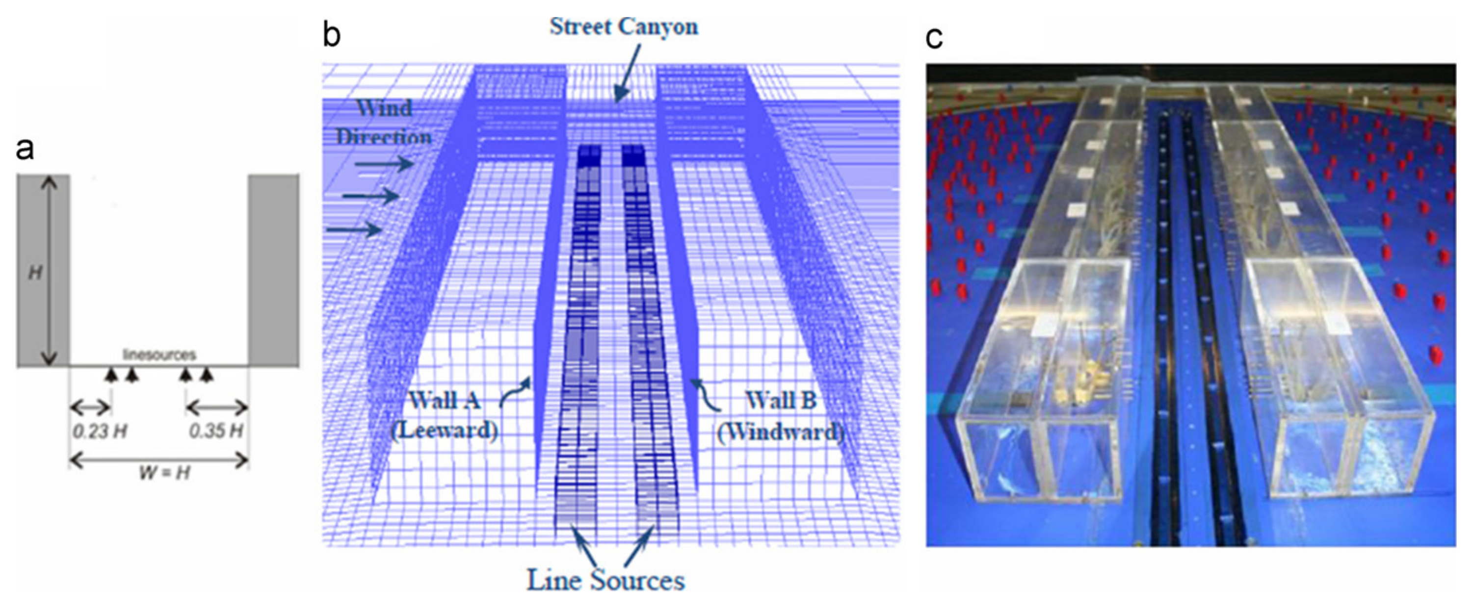
3.1. Setup of Wind-Tunnel Experiment

The experiment was conducted to estimate concentration and flow data in a reduced scale street canyon with an atmospheric boundary layer wind tunnel. An approaching flow with mean velocity ( u ( y ) ) , profile exponent α = 0.3 , and turbulence intensity ( I u ) profile exponent α l = 0.36 , characterized by the power-law approach, were considered in that work. The expressions of these profiles were:
u ( y ) u ( y r e f ) = y y r e f α
and
I u ( y ) I u ( y r e f ) = y y r e f α l
Air velocity u ( y r e f = H ) = 4.65 m s 1 was used. Here, H presents the building height. The works of Gromke and Ruck [18,25] provide broad details on the computational implementation of atmospheric boundary layer flow as well as the information of the integral length scale profile L u x ( y ) and spectral arrangements of turbulent kinetic energy S u u ( y , f ) . A 1:150 scaled design of a separate street canyon of length L = 180 m and street width W = 18 m with two surrounding parallel structures representing buildings of height H = 18 m and width B = 18 m were positioned perpendicular to the approaching flow for the experiment.
Tracer gas emitting from four-line sources blended within the model street and were outlined based on the approach specified in Meroney et al. [27]. They were then used to simulate the discharge of traffic pollutants. The sources passed the street canyon by about 10 % on every side to consider the traffic exhaust discharged in sideways crossings. S F 6 (Sulfur Hexafluoride) was the tracer gas. Mean concentration of the S F 6 was estimated on the canyon walls and was then normalized as follows:
C + = c u H H Q / l
where c is the measured mean concentration, u H is the developed approaching airflow mean velocity at height H, and Q / l is the tracer gas source intensity per unit length.

3.2. Present Simulation Setup

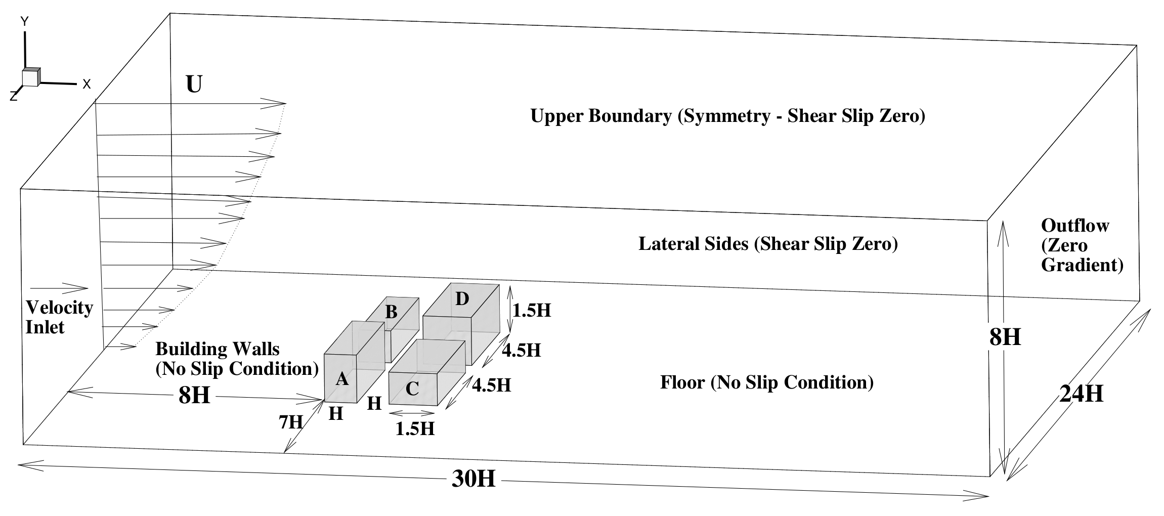
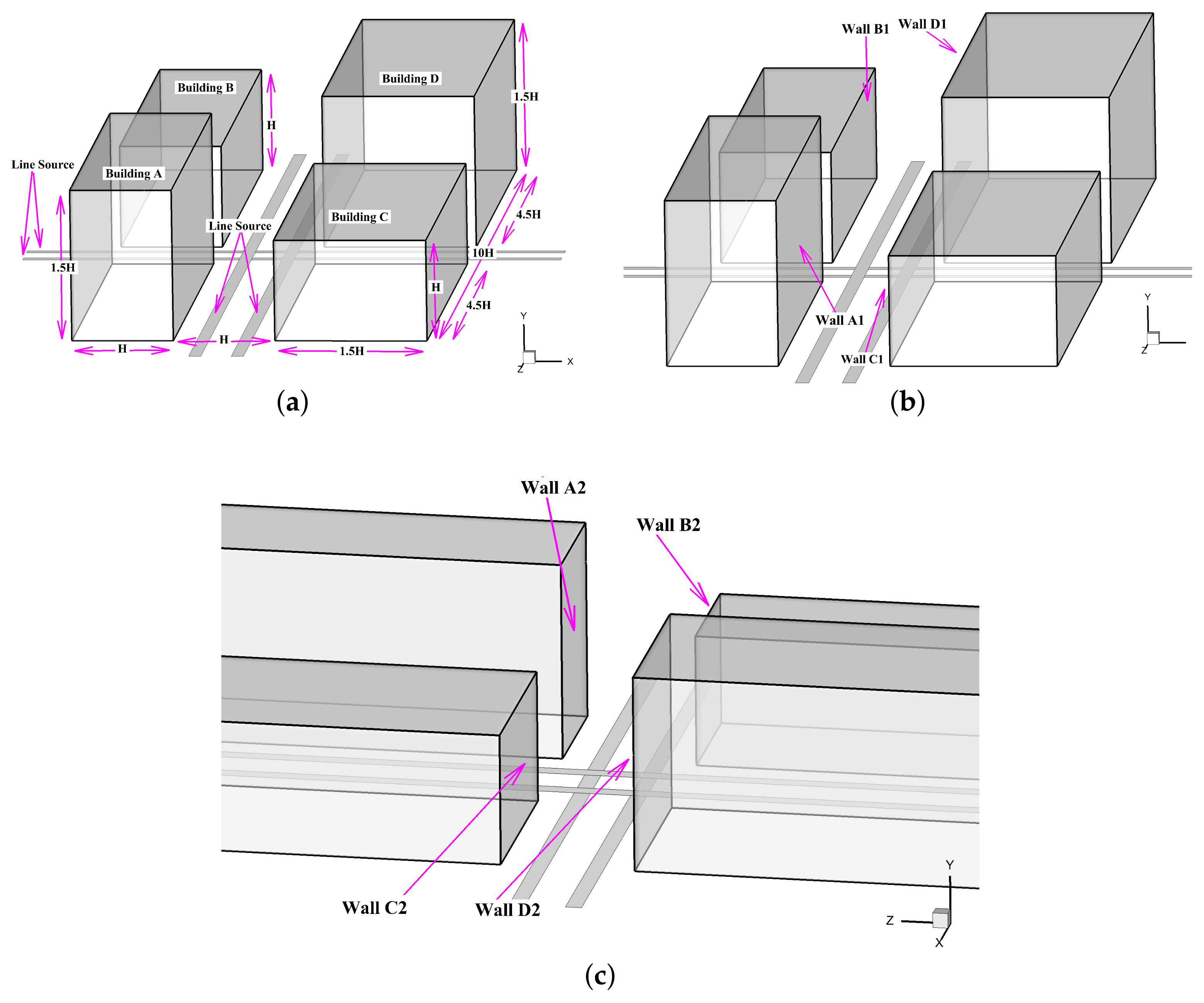
3.2.1. Computational Domain and Boundary Conditions

A large-eddy simulation was carried out using the CFD code ANSYS Fluent™ 15.0 to generate the detailed data of experimental work above, focusing on the pollutant concentrations and flow patterns inside a street canyon. Figure 1 and Figure 2 show the computational domain [28,29,30,31,32,33] and boundary conditions considered in this work. A 1:150 scaled design, similar to the experimental setup, was positioned perpendicular to the approaching flow for the simulation.
Hexahedral elements have been used for the computational domain discretization based on the finite volume method (FVM). A total of 3,015,321 nodes and 2,931,392 cells were used for the simulation. Since the appearance of high gradients in the solution variables, i.e., separation, reattachment, and recirculation, occur in the proximity of the buildings and street canyon, these areas are the region of interest and, therefore, most of the cells were arranged in these regions. The generated mesh has a volume-weighted average orthogonal-quality of 0.998 and skewness of 0.03 ; these values confirm the ‘outstanding’ [34] quality of the mesh.
User-defined functions (UDFs) were executed in the ANSYS Fluent™ to maintain the WT experiment characteristics. The inlet air velocity profile follows the power-law profile of:
u ( y ) = 4.65 y 0.12 0.3 m s 1
The present boundary conditions guarantee the horizontal homogeneity of the turbulent boundary layer [28,29,30,31,32,33,35,36]. The nonexistence of streamwise gradients in the vertical characterizations of mean air velocity and turbulence quantities are termed ‘horizontal homogeneity’, i.e., downstream length is preserved in these characterizations (Blocken et al. [35]). A sand grain roughness, K s , represents the surface roughness in ANSYS Fluent™ rather than the aerodynamic roughness, y 0 . Gromke et al. [36] used K s according to aerodynamic roughness height, y 0 = 0.0033   m in the WT experiment, in order to avoid possible difficulties amidst a coarse grid analysis close to the ground caused by a high sand grain roughness value. Gromke et al. [36] realized that K s being equal to y 0 was not accurate in strong means, yet it was justifiable as it yielded desirable results. The turbulence intensity was low close to the ground ( z / H < 1 ), where changes were less than 10 % . K s = y 0 = 0.0033 m was also set in this work to address the surface roughness. Salim et al. [28,29,30,31,32,33] similarly examined this issue in an ‘empty’ domain.
The ground and building surfaces were treated as smooth walls by default in ANSYS Fluent™, according to the above wall roughness parameters, for the present LES.
The converged time-averaged solution, produced by an unsteady realizable  k ϵ simulation, was synthesized by applying the ANSYS Fluent™’s inbuilt spectral synthesizer in the current LES. This ‘spectral synthesizer’ mechanism follows the characteristics of the work of Smirnov et al. [37]. This practice essentially superimposes turbulence parameters in order to interpret the initial and boundary conditions according to the WT experiment to be applied in the LES.

3.2.2. Flow Simulation

The Smagorinsky–Lilly SGS model with ‘Bounded Central Differencing’ spatial discretization scheme for momentum and ‘Second-Order Upwind’ for species and energy transport equations were applied for this computation. The pressure and pressure–velocity coupling were solved using the ‘Second-Order’ spatial discretization and semi-implicit pressure-linked Equation (SIMPLE) scheme in this work. The present LES considers 10 3 ‘Absolute Criteria’ to address convergence for the scaled residuals.
The time-step size for this simulation is 0.00059 . The volume-weighted average cell convective Courant number, also known as CFL, during the simulation is 0.33 . At first, 77 flow-through computational time (flow-through time is T = L D / U b , where L D is the streamwise length of the domain and U b is the bulk velocity) was calculated in the simulation. The flow reaches a statistical steady-state at this stage. Then, the calculation was carried out for a further 77 flow-through computational time after resetting the initial flow statistics to assure that the decisive time-averaged outcomes were free of the first conditions. The selected 77 flow-through time was compared to the mean solutions of 90 flow-through time in order to check the convergence of the solution. The mean flow field did not vary between these two sampling sizes, additionally confirming that the solution converged.

3.2.3. Dispersion Method

The needed traffic exhaust locations were earmarked in the regions of volume in the geometry and defined as separate fluid zones in order to simulate the line sources. A discharge rate of Q = 10 gs 1 with fluid material S F 6 as the source was then installed for these zones to follow the WT settings. Figure 3 shows more details.

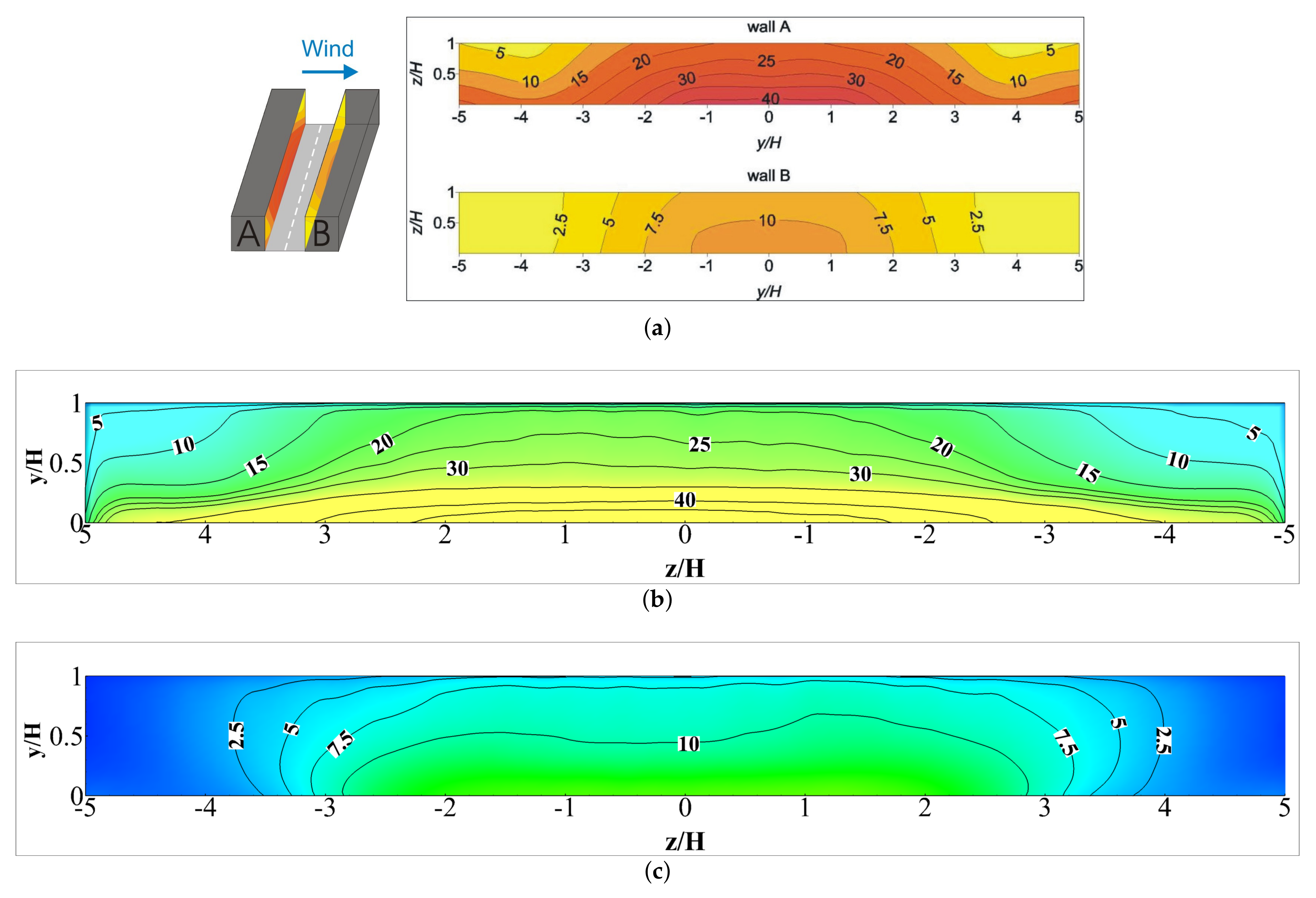
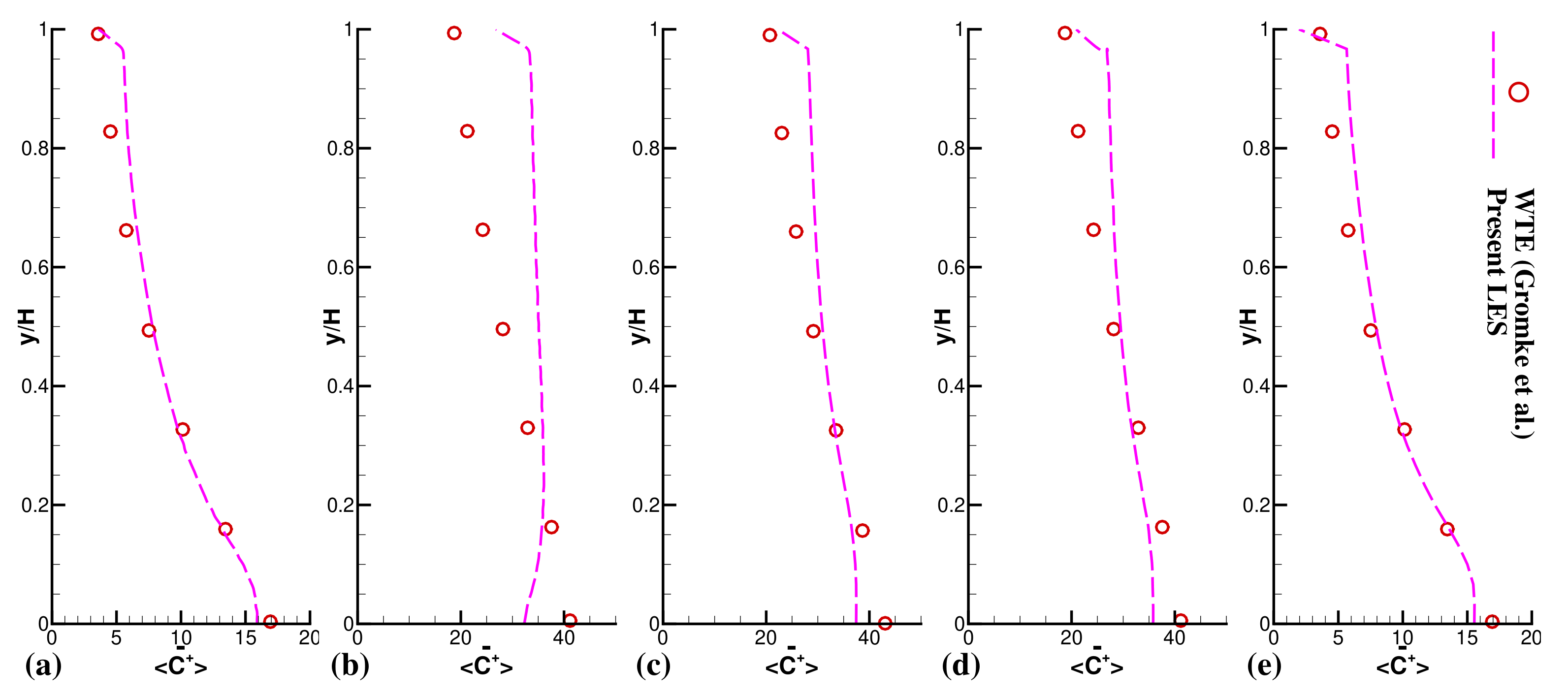
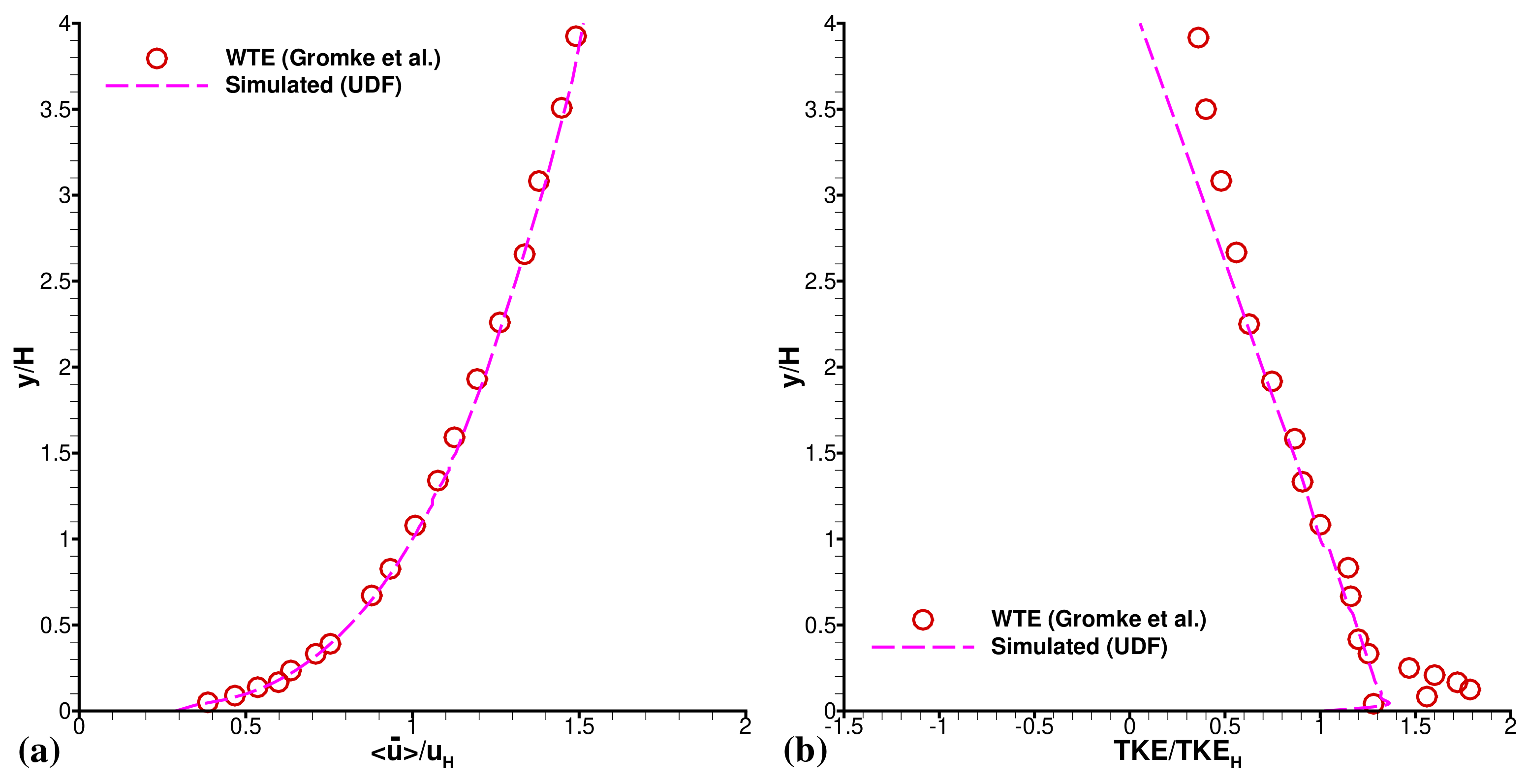
3.2.4. Numerical Validation with Experimental Results for the Street Canyon

Figure 4a–c show the time-averaged normalized pollutant concentration contours at the canyon wall A and wall B. This figure compares the current LES versus the WT estimations. A total of 20 , 000 time-steps were calculated for the present LES time-averaged results following an initial 20 , 000 time-step calculation to reach a steady state. A sampling period of 105   s was considered for the wind tunnel concentration data [18]. It is seen from a qualitative overview of Figure 4 that the present LES can offer efficient results of the spatial pattern of the pollutant. The region of the centre line ( z / H = 0 ) at both walls should be most articulated regarding the concentration pattern, since the highest concentration occurs here and is therefore regarded as the most crucial area.
Figure 5 and Figure 6 graphically show the quantitative representation of pollutant concentration outlines at six various spanwise positions on both walls ( z / H = 0 , z / H = 1.26 , z / H = 1.26 , z / H = 3.79 , z / H = 3.79 ). These figures shows that LES is efficient and steady at projecting the pollutant concentrations at all positions along canyon walls. The WT database does not offer any flow field data. A past study by Salim et al. [29] contained some flow-field and pollutant concentration data along the z / H = 0 line within the street canyon. Salim et al. [29] and several other studies confirmed that LES is the most reliable prediction tool for validating flow fields and turbulence structures in corresponding experiments [28,29,38,39]. It can be noticed from Figure 5 and Figure 6 that the LES prediction of pollutant concentrations at various points of spanwise locations is indeed good.

4. Results and Discussion

4.1. Area of Interest: Dhaka

Dhaka is the capital and the biggest city of Bangladesh. It is the main location for government administration, business, and other industries. Due to the rapid growth and lack of urban planning, environmental and socio-economic problems are increasing [40]. Street canyon intersections in Dhaka see the highest number of traffic compared to any other streets. Most of the street intersections are highly unconventional in design when considering building height and width ratios. That is why an unconventional street intersection design was studied in this work, simplifying the most commonly seen intersection designs in Dhaka, Bangladesh (see Figure 2).
One of the dominant contributors of pollutant dispersion in Dhaka is unfit motor vehicles within narrow streets causing immense traffic congestion. Black carbon (BC) is one of toxic components reported in studies of unfit vehicles in Dhaka. According to Salam et al. [40], the averaged fine particulate matter (FPM) in a typical Dhaka street can go 15 units above the standard value, which raises the temperature into a hot condition even in winter. Therefore, relying on weather conditions is not a realistic approach in terms of street canyons in Dhaka due to the unpredictability of temperatures. While the impact of temperature was reported in the literature, most studies focused on well-developed and planned urban areas in Europe and Australia, for example [41,42]. However, in a city such as Dhaka with almost 21 million people in a 306.4 km 2 area, both roof level and ground level pollutant concentrations need to be monitored concurrently due to the narrow streets and large population.

4.2. Pollutant Concentration Data Overview

The developed numerical method in Section 3 was used to run a simulation considering an urban intersection to analyse pollutant concentrations on the street canyon walls. Figure 2 shows the new building distribution and walls considered for pollutant concentration analysis. A 1:150 scaled design was positioned perpendicular to the approaching flow for the simulation. The validated computational domain [28,29,30,31,32,33] and boundary conditions, described in Figure 1, were considered for this simulation as well.
The meshing method used in the developed numerical strategy, previously discussed in Section 3, was maintained in this simulation. The meshing method generates 2,802,615 nodes and 2,734,066 cells with hexahedral elements. Again, most nodes and cells were generated in the proximity of the buildings and street canyons since these are the areas of interest. Table 1 shows further information of meshes from the ANSYS design module. Meanwhile, the converged time-averaged solutions, referred in Section 3.2.1 are presented in Figure 7 demonstrating for both velocity(Figure 7a) and TKE (Figure 7b) characterisations in the considered inlet boundary conditions. Overall, the correlations between the WTE and UDF for both attributes were found to be in great agreement. Figure 8 shows the grid independence test in terms of the velocity by considering two mesh sets Grid 1 and Grid 2 and found good agreement. Here, Grid 1 was utilized for the whole simulation. The time-step size for this simulation was 0.0018 . The volume-weighted average cell convective Courant number, also known as CFL, during the simulation was 0.89 . Initially, 31 flow-through computational time was calculated to generate time-averaged data. The statistical steady-state was realized at this state. Then, the calculation was sampled for 1, 3, and 5 flow-through computational time after resetting the initial time-averaged flow statistics to demonstrate the time-averaged pollutant concentration evolution for the considered problem. Two more line sources, parallel to the incoming wind flow, were added to the considered model for the current study; more details can be seen in Figure 2. The newly added line sources also maintain the validated dispersion method (see Section 3.2.3) with a discharge rate of Q = 10 gs 1 and S F 6 as the pollutant fluid material.
Figure 9 and Figure 10 present the time-averaged normalized pollutant concentration data at the building walls that were considered for analysis in the modelled urban environment—labelled as A, B, C, and D in Figure 2. A total of 15,000 time-steps were computed for this simulation, maintaining the developed LES method (in Section 3).
Figure 11, Figure 12, Figure 13 and Figure 14 show the evolution of time-averaged normalized concentration data on the canyon walls based on the normalized flow time that was considered for this analysis. These data show that pollutant concentration was initially higher on the walls. Most of the pollutant concentration was close to the ground surface and in the midsection of the walls after the first few normalized flow time points. The wind flow started to come inside the canyons at this stage, and the dispersion of pollutants began. Unchanging dispersion processes, which is the final stage of the pollutant concentration, were observed at the later stages of the flow; the numerical solution converged at this point. By analysing the converged data, it could be seen that the concentration of pollutants was mostly in the area that was closer to the intersection. The pollutant concentration was relatively higher on the section of the street canyon walls closest to the intersection, rather than the walls’ section further from the intersection. This phenomenon is also true for the elevation of the building walls. Therefore, the higher elevation showed lower pollutant concentrations.

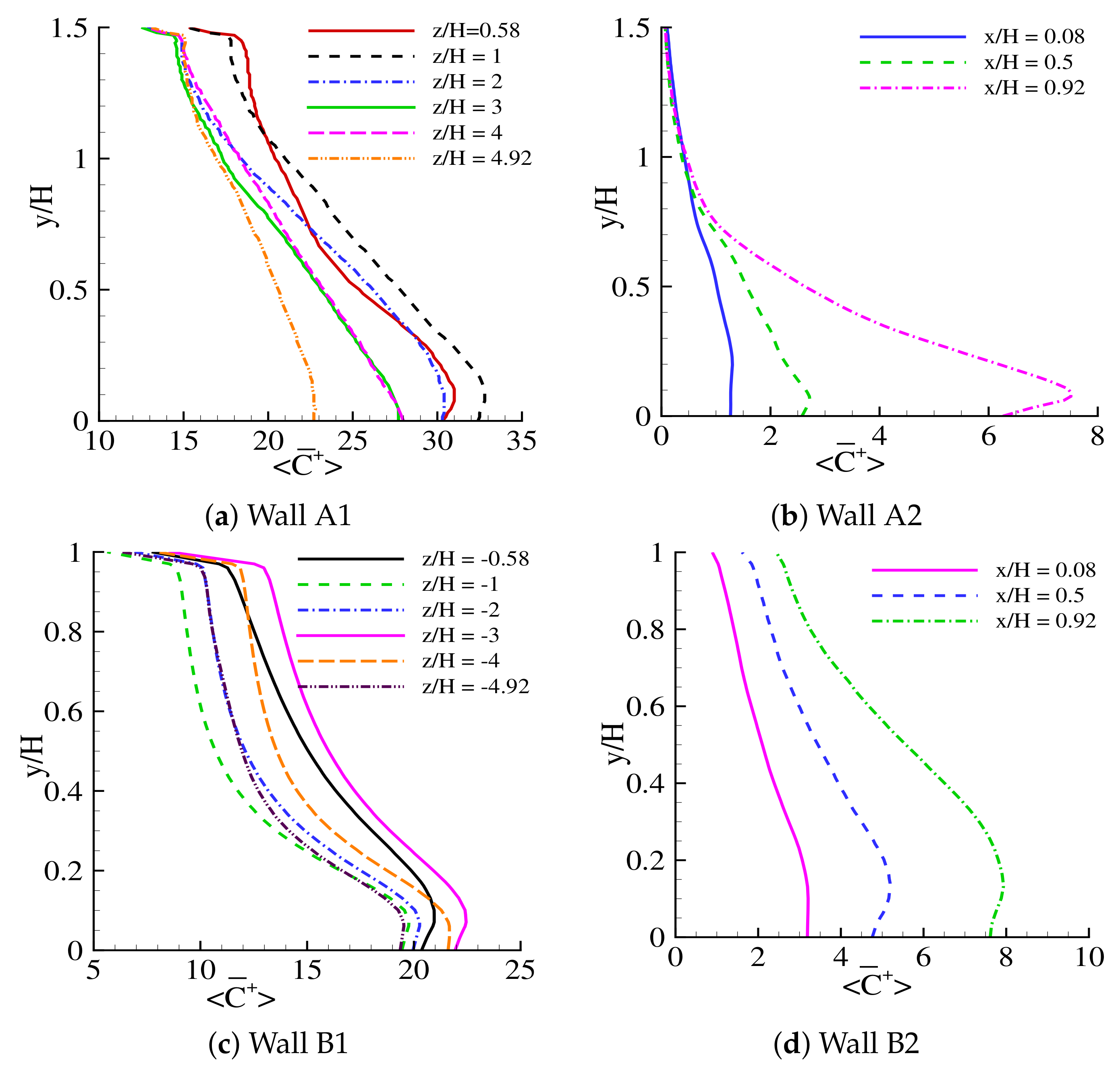
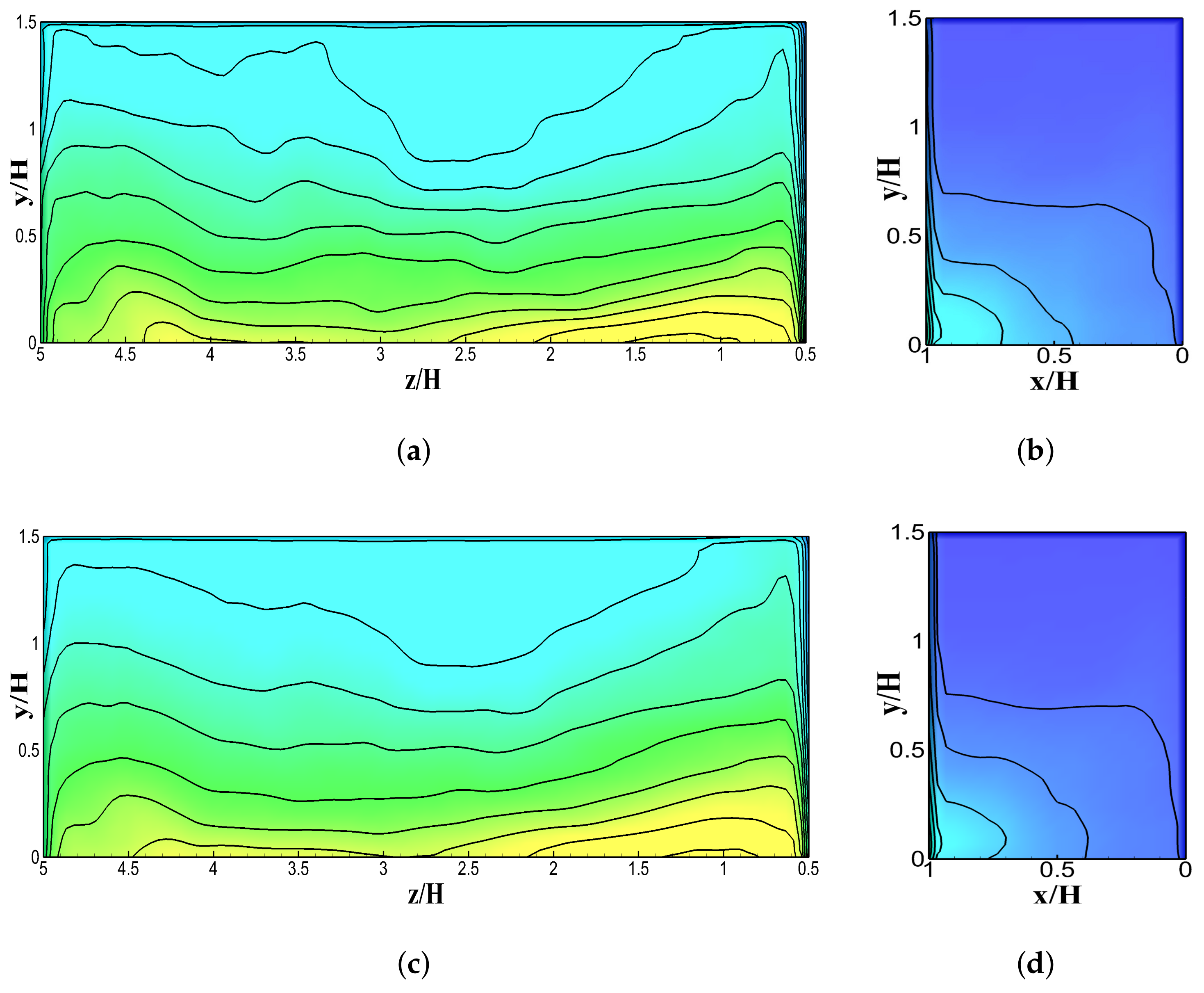
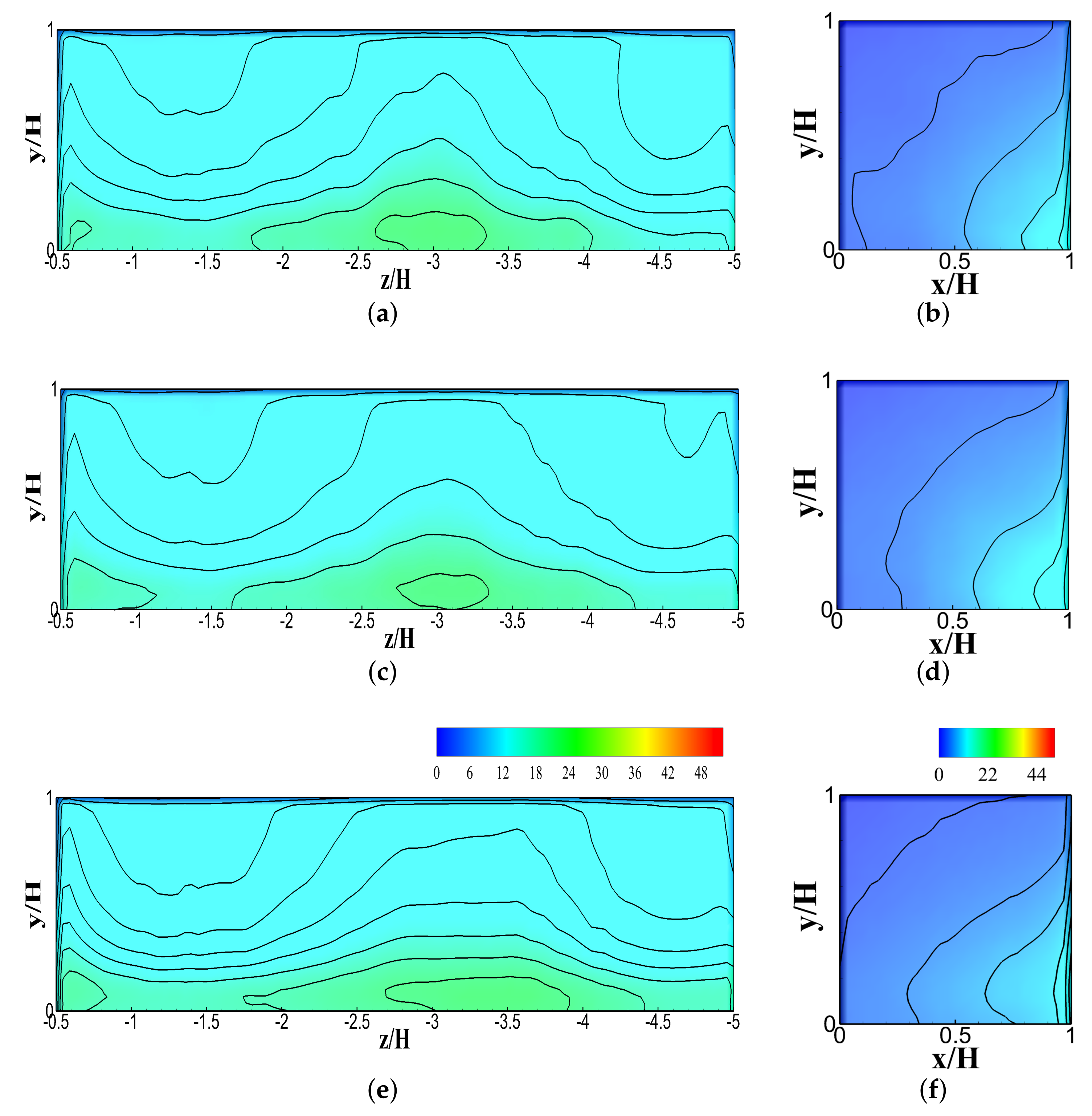
4.3. Pollutant Concentration on Upwind Buildings

Amongst the canyon walls perpendicular to the incoming wind flow, wall A 1 was positioned at the upwind side of the domain and had a relatively higher concentration. Building A had a height of 1.5 H , which is 0.5 H (higher than the reference height (H)). This elevated height prevents the wind from entering or leaving the street canyon (the street canyon between Building A and C) effectively, as can be seen from the streamlines of the velocity magnitude U ¯ / u H in Figure 15 and Figure 16. Both figures further showed that there was not any big circulating vortex in the midsection of the street canyon used to carry the pollutants out of the street canyon, but just a small circulating vortex that formed close to Building A. According to Figure 16, the vertical flow had a relatively low velocity inside the street canyon, thus explaining the higher level of pollutant concentration seen in Figure 11 (Wall A 1 ).
Pollutant concentrations on wall B 1 , also located at the upwind side of the building, were relatively lower compared to those on wall A 1 . The wind flow continuously entered and exited the street canyon (i.e., the street canyon between Buildings B and D) effectively, as seen from the streamlines of the velocity magnitude U ¯ / u H in Figure 15 and Figure 17, since Building B retains the standard reference height of H. Figure 15 and Figure 17 also confirmed the presence of a large circulating vortex inside the street canyon, which is the main factor for pollutant dispersion, along with a smaller vortex formation. The vertical flow velocity had a relatively higher magnitude inside the canyon as seen in Figure 17. The velocity magnitude and vertical velocity data justified the level of pollutant concentration shown in Figure 12 (wall B 1 ).
In the street canyon, two features of the concentration pattern at the inner canyon walls could be observed, as depicted in Figure 4. First, we observed the deterioration of pollutant concentration at the street ending closest to the freeway at both walls A and B. Second, we observed significantly higher concentrations on wall A. However, in the intersection design, the decline in pollutant concentration was not seen for the street ending closest to the intersection; instead the pollutant concentration increased in this area. However, the reduction in concentration was only noticed at the street ending closest to the freeway. Walls A 1 and B 1 , which were perpendicular to the incoming flow, showed a reduced concentration in the intersection design, as described in Figure 9, when compared to wall A in the street canyon. Peak values of concentrations on walls A 1 and B 1 were found to be highly dependent on the heights of Buildings A and B in the intersection design. The drop in the concentrations at the streets ending towards the freeway was the result of improved ventilation for both street canyon and intersection. Nevertheless, in the street intersection design, higher pollutant concentration at the street ending towards the intersection was still evident due to ineffective ventilation.
Walls A 2 and B 2 were situated in the upwind side of the domain, and they were parallel to the incoming wind flow. These two walls had a very low level of pollutant concentrations. Figure 15 showed that the incoming wind mostly flowed through the parallel street canyon (i.e., the small street canyon between Buildings A and B) without any interruption. This flow characteristics explain the level of pollutant concentrations on wall A 2 , as seen in Figure 11 (wall A 2 ).

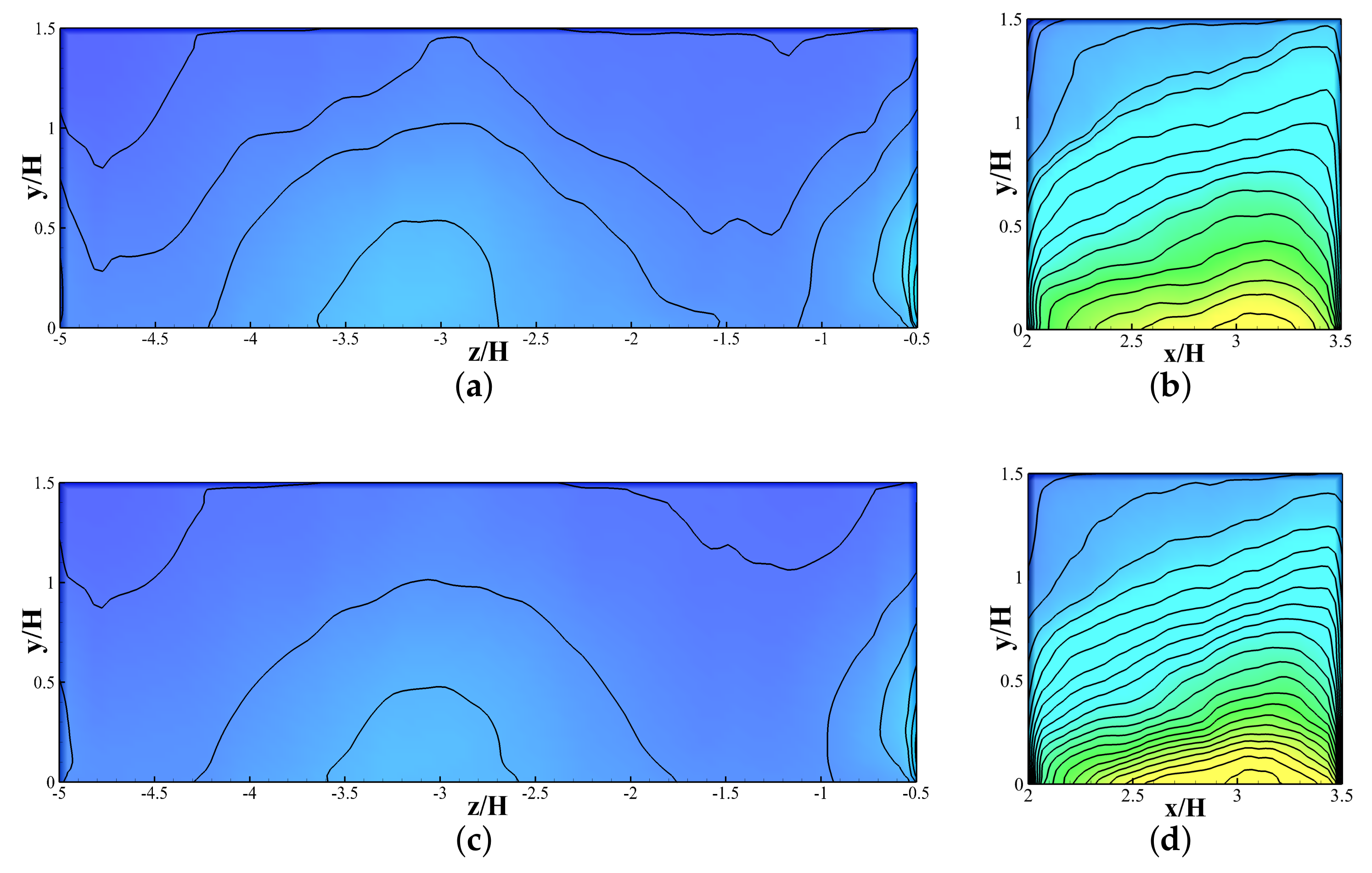
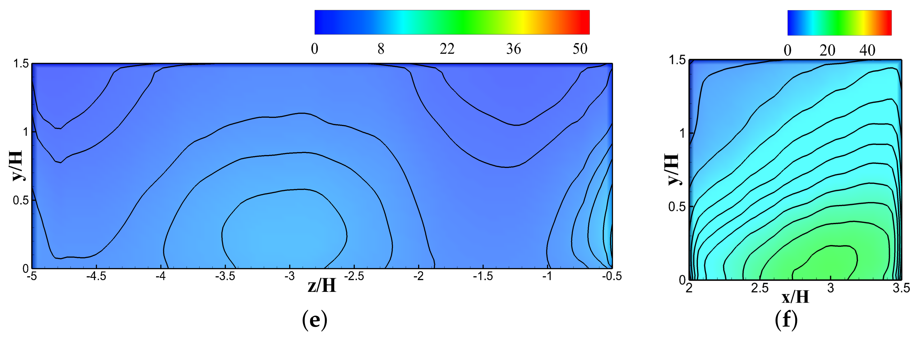
4.4. Pollutant Concentration on Downwind Buildings

As previously described in Section 4.3, upwind Building A had a relatively higher height than the reference height (H). The elevated height causes a poor ventilation facility inside this canyon (i.e., the canyon between Buildings A and C), thus preventing big circulating vortices from developing in this area. Only small vortices were formed inside this canyon, which failed to disperse the traffic-exhaust pollutants effectively. These characteristics of the flow caused a high pollutant concentration on wall C 1 , as shown in Figure 13 (wall C 1 ), even though Building C was situated in the downwind side of the domain. Meanwhile, wall D 1 , also located at the downwind side of the domain, showed the lowest level of pollutant concentration, as shown in Figure 14 (wall D 1 ), compared to other perpendicular street canyon walls even though Building D had a height of 1.5 H , which is 0.5 H higher than the reference height of H. However, this elevation of building D did not prevent the incoming flow from effectively entering or exiting the street canyon (i.e., the canyon between Buildings A and C).
The deterioration in concentration at wall B was seen for the street ending closest to the freeway, as shown in Figure 4, in the street canyon design. However, the downwind side of building wall B showed lower pollutant concentrations when compared to wall A. Furthermore, in the street intersection design, pollutant concentration increased at walls C 1 and D 1 for the street ending closest to the intersection, as seen in Figure 10. The reduction in concentration was also seen on walls C 1 and D 1 for the street ending closest to the freeway. As previously described, this observation proved that the streets ending closest to freeways have much better ventilation facilities when compared to streets ending closest to the intersection. Nonetheless, walls C 1 and D 1 , which are both perpendicular to the incoming flow, had a big difference in pollutant concentrations. As mentioned earlier, in the street canyon design the downwind wall B experienced comparatively lower pollutant concentration. However, in the intersection design wall C 1 experienced a much higher concentration compared to wall D 1 . This behaviour could be attributed to the elevated height of upwind Building A. Nevertheless, compared to the street canyon design, downwind side buildings still see much higher pollutant concentration for the street intersection design due to ineffective ventilation at the street ending closest to the intersection.
The pollutant concentration level on walls C 2 and D 2 was comparatively higher. Building C and D sit on the downwind side of the domain, and have a width of 1.5 H , which is 0.5 H higher than the reference width (H). Before entering the street canyon (i.e., the street canyon between Building B and D) the wind flow was interrupted and separated in several places, as seen in Figure 15. This interruption and separation of the incoming wind flow together with the increased width of theses two buildings have a significant influence on the pollutant concentration level, which explains the relatively higher pollutant concentration level on wall C 2 , as seen in Figure 13 (wall C 2 ), and on wall D 2 , as seen in Figure 14 (wall D 2 ).

5. Discussion on Pollutant Concentration Evolution and Impact

5.1. Sampling Overview

The calculation was sampled at 1, 3, and 5 normalized flow-through computational time points after resetting the initial time-averaged flow statistics in order to demonstrate the time-averaged pollutant concentration evolutions for the considered problem. The sampling was conducted once the statistical steady-state was optimised to illustrate statistical data based on normalised flow instances. This process of capturing pollutant concentration evolution was previously considered for a street canyon [28,29,30,32]. Figure 11, Figure 12, Figure 13 and Figure 14 show these normalized concentration data on the walls considered for analysis.

5.2. Key Findings on Each Building Block

The considered geometry was considered based on four building blocks. Since the position and dimension of the blocks varied in the computation, the key findings on each building block are discussed below.
Building Block A: The peak concentration was larger at initial instances of the normalized flow-time on wall A 1 —seen in Figure 11. After just 1 flow-through time (first instance), the peak concentration was approximately 26.67 % higher compared to the final time-averaged concentration. Wall A 2 showed approximately 33.33 % higher peak concentration after the first instance, compared to the final time-averaged data. The peak concentration was reduced in vertical, streamwise, and spanwise expanses on both walls A 1 and A 2 . The changes in vertical, streamwise, and spanwise extents were significant and noticeable. After the third and fifth instances, the concentration values kept changing, as seen in Figure 11. Every flow-through time (instance) caused the concentration to reduce by dispersing the pollutant, and then the concentration reached the final time-averaged stage when changes were no longer possible.
Building Block B: Wall B 1 showed a high concentration value as anticipated since it was on the leeward side, as seen in Figure 12. This wall also showed a higher concentration after the first instance, and an approximately 66.67 % higher peak concentration compared to the final mean concentration. The third and fifth instances demonstrated approximately 44.44 % and 22.22 % higher peak concentration, respectively. However, vertical and spanwise expanses of the concentration had significantly changed at these points. Wall B 2 had an approximately 33.33 % higher peak concentration, similar to wall A 2 . The changes in vertical and streamwise expanses of the concentration were noticeable for wall B 2 after each instance (third and fifth) compared to the first instance.
Building Block C: Wall C 1 , even though it was on the windward side, experienced a high pollutant concentration, as displayed in Figure 13. In initial instances, and at the first, third, and fifth instances, it showed an approximately 63.64 % , 59.09 % , and 54.5 % higher peak concentration compared to the final mean concentration, respectively. Furthermore, wall C 2 showed up to an approximately 42.86 % higher peak concentration in initial instances. In addition, similar every other wall, these two walls exhibited changes in pollutant concentration in vertical, streamwise, and spanwise expanses.
Building Block D: Wall D 1 , which was on the windward side, demonstrated a low pollutant concentration overall, as shown in Figure 14. This relatively lower concentration was in line with the initial hypothesis and similar to the windward wall of the street canyon. The lower concentration values were seen from the first instance. However, the peak concentration was still approximately 50 % higher compared to the final mean concentration. Although the distribution of the concentration changes after the third instance, the peak concentration still remained approximately 50 % higher compared to the final mean value. After the fifth instance, the peak concentration stayed approximately 25 % higher. However, wall D 2 shows a different pattern compared to other walls. The maximum difference of peak concentration was 58.33 % higher compared to final mean concentration. This was seen after the third instance before the peak concentration started decreasing again. Similar to the other walls, walls D 1 and D 2 showed changes in pollutant concentration in vertical, streamwise, and spanwise expanses in every instance.

5.3. Significance of the Approach and Future Directions

The demand for understanding the pollutant dispersion in the presence of an unconventional adjacent street canyon should serve as a realistic yardstick rather than a simplified urban street design with fixed aspect ratios. The profitability of the template pollutant dispersion design presented in this study should benefit inhabitants of densely-populated urban area such as Dhaka. As a result, if the pollutant concentration can be monitored through an automated model based on concentration level monitoring, a proper urbanization of a city can be implemented for the benefit of human beings. The pollutant concentration values including the peaks and the rate of plummeting reported in this study should be useful for analysing the ’building geometry’ and its impact on airflow. Having access to pollutant concentration data on a regular basis, air quality control professionals could liaise with councils or property owners to understand the separation of buildings or walls including an in-depth understanding of height and width. As previously mentioned, most of the published works were based on geometries of urban buildings in terms of roof-level concentration monitoring and were based on geographic location. This finding makes sense to some extent. However, in a place such as Dhaka where traffic congestion is quite familiar in any commercial area, the street-level pollutant concentration needs to be considered. In addition, this could help air quality researchers in Dhaka create a map (similar to ESRI ArcGIS or Google Earth) to record and create a database for Dhaka’s pollutant concentrations at both roof and street levels. Bangladesh working on becoming fully digital to benefit citizens through the programme “Bangladesh Vision 2041”, where a smartphone application could be developed and made available for everyone for live air quality monitoring [43,44]. Therefore, a range of parametric modelling was implemented while developing this model, such as varying the aspect ratio, timescale, and grid/node size of the numerical simulations, and the conclusion on the peak concentration was reached. This will help provide significantly more information to urban dwellers or any other concerned citizen.
Based on the findings of the current study and the literature review, adequate evidence now exists to definitely emphasize the potential of the adjacent street canyon model into commercial applications or improvement of existing applications. Even in a developed country such as Australia, the Environment Protection Authority (EPA) Victoria often finds it difficult to track air pollutant concentration at a large scale in the state of Victoria [45,46]. The process would also replace the manual labour required to monitor the concentration levels at a short timescale because the changes in pollutant concentration would be recorded automatically through the model. While a specific area of interest was considered in this study, there is a room for improvement across a larger region with the possible implications of geographical coordinates. This process is already in practice in developed countries, but it should find future applications in Bangladesh.

6. Conclusions

Atmospheric flow and pollutant dispersion processes inside a conventional urban street canyon and a novel model urban intersection were presented in this study. At first, numerical computations were performed for the urban street canyon, and the obtained results were compared with previous wind tunnel experiments. The validated numerical method was applied later in order to carry out a numerical study for a model urban intersection. The presence of an unconventional adjacent street canyon forming a street intersection is one of the unique features of this study. The numerical calculation was sampled at one, three, and five normalized flow through time points. Prior to that, the initial time-averaged flow statistics were reset to explain the evolution of pollutant concentration within the considered geometry. For the considered urban intersection, the parts close to the urban-intersection always showed the maximum concentrations. Increasing the height of a building in the upwind side of the domain prevents flows to come inside of the A–C perpendicular street canyon and form strong canyon vortices, which essentially led to ineffective pollutant dispersion inside this street canyon. It was also observed that the highest pollutant concentration by wall A1 and A2 exhibited approximately 26.67 % and 33.33 % increases at the first instance compared to the final time-averaged concentration. Furthermore, wall B2 demonstrated an identical increase to wall A2 ( 33.33 % ), whereas the peak concentration at wall B1 showed a sharp increase of 66.67 % after the first instance. The rate of increase plummeted to 44.44 % and 22.22 % after the third and fifth instances. Increased width of buildings in the downwind side of the domain also causes a high pollutant concentration inside of C–D parallel street canyon. Interestingly, the maximum pollutant concentrations at wall C1 after first, third, and fifth instances remained quite close to 63.64 % , 59.09 % , and 54.5 % , respectively, whereas wall C2 initially recorded an almost 42.86 % increase in the concentration, which is much greater than that of walls A2 and B2. Unlike the other walls, D demonstrated a lower pollutant concentration after the fifth instance (only 25 % higher than the initial). Furthermore, it was also proven that unbalanced natural ventilation inside the street canyons worked as a catalyst for largely increasing the pollutant concentrations at the pedestrian level and on the street canyon walls. The importance of the height and width of buildings in the upwind side of the domain, considering the reference height H and width W, was cemented through numerical work that showed how the canyon vortex or canyon vortex-like structures were likely to develop. Over-height buildings, in the upwind side of the domain, block the flow entering into the canyon and thus fail to remove the polluted air. The findings of this research were found to be in accordance with this conceptual understanding as well.
The key findings of this study suggest that the 3D interconnection between dominating canyon vortices and roof level flow determine the pollutant concentration level on windward walls. Therefore, the extent of corner eddies and associated correlations with dominating vortices are responsible for enhanced ventilation. The flow structures and concentration profiles observed in the present study can be further analyzed and improved, particularly those identifying changes such as the presence of trees in the canyons. Ordinarily, numerical modelling considers porous structures to simulate trees in pollutant dispersion studies. More investigations on the flow and concentration profiles of the considered model urban intersection with tree plating inside the canyon’s together with the appropriate numerical method, would be of interest in order to broaden this knowledge.

Author Contributions

Conceptualization, S.H., P.N., M.M.M., A.K. and M.F.H.; methodology, P.N., M.M.M. and A.K.; software, A.K.; validation, S.H.; formal analysis, S.H. and U.H.A.; investigation, S.H. and U.H.A.; resources, P.N., M.M.M., A.K. and M.F.H.; data curation, U.H.A.; writing—original draft preparation, S.H.; writing—review and editing, U.H.A., P.N., M.M.M., A.K. and M.F.H.; visualization, S.H.; supervision, M.M.M.; project administration, P.N., M.M.M., A.K. and M.F.H.; funding acquisition, M.M.M. All authors have read and agreed to the published version of the manuscript.

Funding

The first four authors gratefully acknowledge the Ministry of Education, Government of Bangladesh, for providing financial support (Grant No.:MS20191054). The fourth author gratefully acknowledges North South University for financial support via a faculty research grant (Grant No.: CTRG-21-SEPS-12).

Institutional Review Board Statement

Not applicable.

Informed Consent Statement

Not applicable.

Data Availability Statement

The data are available based on reasonable request.

Acknowledgments

All the authors gratefully acknowledge the fifth author and the University of Leeds for providing the facilities needed to use ANSYS Fluent.

Conflicts of Interest

The authors declare no conflict of interest.

Nomenclature

English Symbol
BBuilding width
cMeasured mean concentration
C + Normalized pollutant concentration
C ¯ + Mean normalized pollutant concentration
C ¯ + Sampled mean normalized pollutant concentration
C s Smagornisky constant
dDistance to the nearest wall
DDomain of the fluid
D t Turbulent diffusivity
GFilter function
h s Sensible enthalpy
HBuilding height
I u Turbulence intensity
kTurbulent kinetic energy
K s Sand grain roughness height
k T Thermal conductivity in terms of species transport
lTracer gas source length
LLength of street canyon
L D Streamwise length of the domain
L s Mixing length of sub-grid-scales
L u x Integral length scale profile
L e i Lewis number
M s g s Sub-grid-scale Mach number
NTotal number of fluid phase chemical species considered in the problem
P r S G S Sub-grid-scale Prandtl number
q j Sub-grid-scale flux
QTracer gas intensity
Q v c Vortex core structure method Q-criterion
R i Rate of generation of species
R e Reynolds number
S i Rate of generation due to addition from the dispersed state and any UDS
S ¯ i j Rate-of-strain tensor
S u u Spectral arrangements of turbulent kinetic energy
S c t Turbulent Schmidt number
TFlow-through time
uStreamwise velocity
u ¯ Mean streamwise velocity
u ¯ Sampled mean streamwise velocity
u H Developed approaching airflow mean velocity at height H
UVelocity magnitude
U ¯ Mean velocity magnitude
U ¯ Sampled mean velocity magnitude
U b Bulk velocity
vVertical velocity
v ¯ Mean vertical velocity
v ¯ Sampled mean vertical velocity
VVolume of a computational cell
wSpanwise velocity
w ¯ Mean spanwise velocity
w ¯ Sampled mean spanwise velocity
WStreet-canyon width
xLength in x-direction
yLength in y-direction
y 0 Aerodynamic roughness height
Y i Local mass fraction of the species
zLength in z-direction
Greek Symbol    
α Mean velocity profile exponent
α l Turbulence intensity profile exponent
Δ Bounded grid-scale
ϵ Turbulent dissipation rate
κ Von Kármán constant
λ Thermal conductivity
μ S G S Sub-grid-scale viscosity
μ t Sub-grid-scale turbulent viscosity
σ i j Stress tensor because of molecular viscosity
τ i j Sub-grid-scale stress
τ k k Isotropic component of sub-grid-scale stress
ϕ ˜ Density-weighted (or Favre) filtering term

References

  1. Li, X.X.; Liu, C.H.; Leung, D.Y. Large-eddy simulation of flow and pollutant dispersion in high-aspect-ratio urban street canyons with wall model. Bound.-Layer Meteorol. 2008, 129, 249–268. [Google Scholar] [CrossRef]
  2. Chen, G.; Wang, D.; Wang, Q.; Li, Y.; Wang, X.; Hang, J.; Gao, P.; Ou, C.; Wang, K. Scaled outdoor experimental studies of urban thermal environment in street canyon models with various aspect ratios and thermal storage. Sci. Total Environ. 2020, 726, 138147. [Google Scholar] [CrossRef] [PubMed]
  3. García, M.Á.; Pérez, I.A. Lower Atmosphere Meteorology. Atmosphere 2019, 10, 609. [Google Scholar] [CrossRef] [Green Version]
  4. Buccolieri, R.; Gatto, E.; Manisco, M.; Ippolito, F.; Santiago, J.L.; Gao, Z. Characterization of urban greening in a district of Lecce (Southern Italy) for the analysis of CO2 storage and air pollutant dispersion. Atmosphere 2020, 11, 967. [Google Scholar] [CrossRef]
  5. Ming, T.; Fang, W.; Peng, C.; Cai, C.; De Richter, R.; Ahmadi, M.H.; Wen, Y. Impacts of traffic tidal flow on pollutant dispersion in a non-uniform urban street canyon. Atmosphere 2018, 9, 82. [Google Scholar] [CrossRef] [Green Version]
  6. Yuan, C.; Shan, R.; Zhang, Y.; Li, X.X.; Yin, T.; Hang, J.; Norford, L. Multilayer urban canopy modelling and mapping for traffic pollutant dispersion at high density urban areas. Sci. Total Environ. 2019, 647, 255–267. [Google Scholar] [CrossRef]
  7. Hassan, S.; Molla, M.; Nag, P.; Akhter, N.; Khan, A. Unsteady RANS simulation of wind flow around a building shape obstacle. In Building Simulation; Springer: Berlin/Heidelberg, Germany, 2022; Volume 15, pp. 291–312. [Google Scholar]
  8. Himika, T.A.; Hasan, F.; Molla, M. Lattice Boltzmann simulation of airflow and mixed convection in a general ward of hospital. J. Comput. Eng. 2016, 2016, 5405939. [Google Scholar] [CrossRef] [Green Version]
  9. Hasan, M.F.; Ahmed Himika, T.; Molla, M.M. Lattice Boltzmann simulation of airflow and heat transfer in a model ward of a hospital. J. Therm. Sci. Eng. Appl. 2017, 9, 011011. [Google Scholar] [CrossRef]
  10. Walton, A.; Cheng, A. Large-eddy simulation of pollution dispersion in an urban street canyon—Part II: Idealised canyon simulation. Atmos. Environ. 2002, 36, 3615–3627. [Google Scholar] [CrossRef]
  11. Zhiyin, Y. Large-eddy simulation: Past, present and the future. Chin. J. Aeron. 2015, 28, 11–24. [Google Scholar] [CrossRef] [Green Version]
  12. Hasan, M.F.; Himika, T.A.; Molla, M.M. Large-eddy simulation of airflow and heat transfer in a general ward of hospital. AIP Conf. Proc. 2016, 1754, 050022. [Google Scholar]
  13. Smagorinsky, J. General circulation experiments with the primitive equations: I. The basic experiment. Mon. Weather Rev. 1963, 91, 99–164. [Google Scholar] [CrossRef]
  14. Son, M.; Lee, J.I.; Kim, J.J.; Park, S.J.; Kim, D.; Kim, D.Y. Evaluation of the Wind Environment around Multiple Urban Canyons Using Numerical Modeling. Atmosphere 2022, 13, 834. [Google Scholar] [CrossRef]
  15. Salim, S.; Ong, K.; Cheah, S. Comparison of RANS, URANS and LES in the Prediction of Airflow and Pollutant Dispersion. Proc. World Cong. Eng. Comput. Sci. 2011, 2, 19–21. [Google Scholar]
  16. Zhang, Y.; Gu, Z.; Yu, C.W. Impact factors on airflow and pollutant dispersion in urban street canyons and comprehensive simulations: A review. Curr. Pollut. Rep. 2020, 6, 425–439. [Google Scholar] [CrossRef]
  17. Gromke, C.; Denev, J.; Ruck, B. Dispersion of traffic exhausts in urban street canyons with tree plantings-experimental and numerical investigations. In Proceedings of the International Workshop on Physical Modelling of Flow and Dispersion Phenomena (PHYSMOD 2007), Orleans, France, 23–25 August 2007; Volume 1. [Google Scholar]
  18. Gromke, C.; Ruck, B. Influence of trees on the dispersion of pollutants in an urban street canyon—Experimental investigation of the flow and concentration field. Atmos. Environ. 2007, 41, 3287–3302. [Google Scholar] [CrossRef] [Green Version]
  19. Gromke, C.; Ruck, B. Flow and dispersion phenomena in urban street canyons in the presence of trees. In Proceedings of the 12th International Conference on Wind Engineering, Cairns, Australia, 1–6 July 2007. [Google Scholar]
  20. Gromke, C.; Ruck, B. On the impact of trees on dispersion processes of traffic emissions in street canyons. Bound.-Layer Meteorol. 2009, 131, 19–34. [Google Scholar] [CrossRef]
  21. Gromke, C.; Jamarkattel, N.; Ruck, B. Influence of roadside hedgerows on air quality in urban street canyons. Atmos. Environ. 2016, 139, 75–86. [Google Scholar] [CrossRef]
  22. Gadde, S.N.; Stieren, A.; Stevens, R.J. Large-eddy simulations of stratified atmospheric boundary layers: Comparison of different subgrid models. Bound.-Layer Meteorol. 2021, 178, 363–382. [Google Scholar] [CrossRef]
  23. Hasan, M.F.; Molla, M.; Kamrujjaman, M.; Siddiqa, S. Natural Convection Flow over a Vertical Permeable Circular Cone with Uniform Surface Heat Flux in Temperature-Dependent Viscosity with Three-Fold Solutions within the Boundary Layer. Computation 2022, 10, 60. [Google Scholar] [CrossRef]
  24. Wang, S.; De Roo, F.; Thobois, L.; Reuder, J. Characterization of Terrain-Induced Turbulence by Large-Eddy Simulation for Air Safety Considerations in Airport Siting. Atmosphere 2022, 13, 952. [Google Scholar] [CrossRef]
  25. Gromke, C.; Ruck, B. Effects of trees on the dilution of vehicle exhaust emissions in urban street canyons. Int. J. Environ. Waste Manag. 2009, 4, 225–242. [Google Scholar] [CrossRef]
  26. Hinze, J. Turbulence; McGraw-Hill Publishing Co.: New York, NY, USA, 1975. [Google Scholar]
  27. Meroney, R.N.; Leitl, B.M.; Rafailidis, S.; Schatzmann, M. Wind-tunnel and numerical modeling of flow and dispersion about several building shapes. J. Wind Eng. Indust. Aerodyn. 1999, 81, 333–345. [Google Scholar] [CrossRef]
  28. Salim, S.M.; Chan, A.; Buccolieri, R.; Di Sabatino, S. CFD Study on the Roles of Trees on Airflow and Pollutant Dispersion within Urban Street Canyons. In CFD Applications in Energy and Environmental Sectors; International Energy and Environmental Foundation: Tripoli, Libya, 2011; pp. 175–204. [Google Scholar]
  29. Salim, S.M.; Buccolieri, R.; Chan, A.; Di Sabatino, S. Numerical simulation of atmospheric pollutant dispersion in an urban street canyon: Comparison between RANS and LES. J. Wind Eng. Indust. Aerodyn. 2011, 99, 103–113. [Google Scholar] [CrossRef]
  30. Salim, S.M.; Cheah, S.C.; Chan, A. Numerical simulation of dispersion in urban street canyons with avenue-like tree plantings: Comparison between RANS and LES. Build. Environ. 2011, 46, 1735–1746. [Google Scholar] [CrossRef]
  31. Ng, W.Y.; Chau, C.K. A modeling investigation of the impact of street and building configurations on personal air pollutant exposure in isolated deep urban canyons. Sci. Total Environ. 2014, 468, 429–448. [Google Scholar] [CrossRef] [PubMed]
  32. Kwa, S.; Salim, S. Numerical Simulation of Dispersion in an Urban Street Canyon: Comparison between Steady and Fluctuating Boundary Conditions. Eng. Lett. 2015, 23. [Google Scholar]
  33. Vranckx, S.; Vos, P.; Maiheu, B.; Janssen, S. Impact of trees on pollutant dispersion in street canyons: A numerical study of the annual average effects in Antwerp, Belgium. Sci. Total Environ. 2015, 532, 474–483. [Google Scholar] [CrossRef]
  34. Lachance-Barrett, S.; Alexander, K. Wind Turbine Blade FSI (Part 1)—Mesh; Cornell University: Ithaca, NY, USA, 2018. [Google Scholar]
  35. Blocken, B.; Carmeliet, J.; Stathopoulos, T. CFD evaluation of wind speed conditions in passages between parallel buildings—effect of wall-function roughness modifications for the atmospheric boundary layer flow. J. Wind Eng. Indust. Aerodyn. 2007, 95, 941–962. [Google Scholar] [CrossRef]
  36. Gromke, C.; Buccolieri, R.; Di Sabatino, S.; Ruck, B. Dispersion study in a street canyon with tree planting by means of wind tunnel and numerical investigations–evaluation of CFD data with experimental data. Atmos. Environ. 2008, 42, 8640–8650. [Google Scholar] [CrossRef]
  37. Smirnov, A.; Shi, S.; Celik, I. Random flow generation technique for large eddy simulations and particle-dynamics modeling. J. Fluids Eng. 2001, 123, 359–371. [Google Scholar] [CrossRef]
  38. Moonen, P.; Dorer, V.; Carmeliet, J. Large Eddy Simulation of concentration fluctuations in an urban street canyon. In Proceedings of the 7th International Colloquium on Bluff Body Aerodynamics, Shanghai, China, 2–6 September 2012. [Google Scholar]
  39. Merlier, L.; Jacob, J.; Sagaut, P. Lattice-Boltzmann Large-Eddy Simulation of pollutant dispersion in street canyons including tree planting effects. Atmos. Environ. 2018, 195, 89–103. [Google Scholar] [CrossRef] [Green Version]
  40. Salam, A.; Andersson, A.; Jeba, F.; Haque, M.I.; Hossain Khan, M.D.; Gustafsson, O. Wintertime air quality in megacity Dhaka, Bangladesh strongly affected by influx of black carbon aerosols from regional biomass burning. Environ. Sci. Technol. 2021, 55, 12243–12249. [Google Scholar] [CrossRef]
  41. Santamouris, M.; Papanikolaou, N.; Koronakis, I.; Livada, I.; Asimakopoulos, D. Thermal and air flow characteristics in a deep pedestrian canyon under hot weather conditions. Atmos. Environ. 1999, 33, 4503–4521. [Google Scholar] [CrossRef]
  42. Huang, Y.; Lei, C.; Liu, C.H.; Perez, P.; Forehead, H.; Kong, S.; Zhou, J.L. A review of strategies for mitigating roadside air pollution in urban street canyons. Environ. Pollut. 2021, 280, 116971. [Google Scholar] [CrossRef]
  43. Hasan, M.M.; Chongbo, W. Estimating energy-related CO2 emission growth in Bangladesh: The LMDI decomposition method approach. Energy Strategy Rev. 2020, 32, 100565. [Google Scholar] [CrossRef]
  44. Islam, A.; Ahmed, M.T.; Mondal, M.A.H.; Awual, M.R.; Monir, M.U.; Islam, K. A snapshot of coal-fired power generation in Bangladesh: A demand–supply outlook. In Natural Resources Forum; Wiley Online Library: Oxford, UK, 2021; Volume 45, pp. 157–182. [Google Scholar]
  45. Hurley, P.; Manins, P.; Lee, S.; Boyle, R.; Ng, Y.L.; Dewundege, P. Year-long, high-resolution, urban airshed modelling: Verification of TAPM predictions of smog and particles in Melbourne, Australia. Atmos. Environ. 2003, 37, 1899–1910. [Google Scholar] [CrossRef]
  46. Sinnott, R.O.; Wang, Y.; Wang, Y. Real-time Route Planning using Mobile Air Pollution Detectors and Citizen Scientists. In Proceedings of the 2021 17th International Conference on Wireless and Mobile Computing, Networking and Communications (WiMob), Bologna, Italy, 11–13 October 2021; IEEE: Piscataway, NJ, USA, 2021; pp. 139–144. [Google Scholar]
Figure 1. Computational domain and boundary conditions for numerical simulation.
Atmosphere 13 01028 g001
Figure 2. A model street canyon intersection: (a) building distribution, (b) walls 1, and (c) walls 2.
Atmosphere 13 01028 g002
Figure 3. Illustrations on geometries and zones: (a) Outline of the locations of line sources inside the street canyon and the line sources presented for the (b) Computational Domain and (c) wind tunnel setup [17,18,19,20] ©CODASC, KIT, https://www.umweltaerodynamik.de/bilder-originale/CODA/CODASC.html (accessed on 20 June 2022).
Atmosphere 13 01028 g003
Figure 4. Time-averaged normalized pollutant concentration C ¯ + data on wall A (leeward) and wall B (windward) presenting comparison of current LES vs. WT Experiment. (a) Wind tunnel experiment data [17,18,19,20] ©CODASC, KIT, https://www.umweltaerodynamik.de/bilder-originale/CODA/CODASC.html (accessed on 20 June 2022); (b) wall A for present LES; (c) wall B for present LES.
Atmosphere 13 01028 g004
Figure 5. Time-averaged normalized pollutant concentration C ¯ + profiles at five separate spanwise positions on wall A, (a) z / H = 3.79 ; (b) z / H = 1.26 ; (c) z / H = 0 ; (d) z / H = 1.26 ; (e) z / H = 3.79 ; to compare current LES vs. WT Experiment.
Atmosphere 13 01028 g005
Figure 6. Time-averaged normalized pollutant concentration C ¯ + profiles at five separate spanwise positions on wall B, (a) z / H = 3.79 ; (b) z / H = 1.26 ; (c) z / H = 0 ; (d) z / H = 1.26 ; (e) z / H = 3.79 ; to compare current LES vs. WT Experiment.
Atmosphere 13 01028 g006
Figure 7. Characterisations in the inlet boundary condition for (a) Velocity and (b) TKE, presenting a comparison of the simulated characterisations produced by applying UDFs with the experimental characterisations.
Atmosphere 13 01028 g007
Figure 8. Grid independence test: velocity distributions for y / H = 0.5 .
Atmosphere 13 01028 g008
Figure 9. Time-averaged normalized concentration C ¯ + data on (a,b) walls A and (c,d) walls B (upwind buildings).
Atmosphere 13 01028 g009
Figure 10. Time-averaged normalized concentration C ¯ + data on (a,b) walls C and (c,d) walls D (downwind buildings).
Atmosphere 13 01028 g010
Figure 11. Evolution of time-averaged normalized concentration C ¯ + data on Building A (upwind building) based on normalized flow time: (a) Wall A1, after 3 flow time; (b) Wall A2, after 3 flow time; (c) Wall A1, after 5 flow time; (d) Wall A2, after 5 flow time; (e) Wall A1 at the final stage; and (f) Wall A2, at the final stage.
Atmosphere 13 01028 g011aAtmosphere 13 01028 g011b
Figure 12. Evolution of time-averaged normalized concentration C ¯ + data on Building B (upwind building) based on normalized flow time: (a) Wall B1 after 3 flow times; (b) wall B2 after 3 flow times; (c) wall B1 after 5 flow times; (d) wall B2 after 5 flow times; (e) wall B1 at the final stage; (f) wall B2 at the final stage.
Atmosphere 13 01028 g012
Figure 13. Evolution of time-averaged normalized concentration C ¯ + data on Building C (downwind building) based on normalized flow time: (a) Wall C1 after 3 flow times; (b) Wall C2 after 3 flow times; (c) Wall C1 after 5 flow times; (d) Wall C2 after 5 flow times; (e) Wall C1 at the final stage; (f) Wall C2 at the final stage.
Atmosphere 13 01028 g013
Figure 14. Evolution of time-averaged normalized concentration C ¯ + data on Building D (downwind building) based on normalized flow time: (a) Wall D1 after 3 flow times; (b) Wall D2 after 3 flow times; (c) Wall D1 after 5 flow timse; (d) Wall D2 after 5 flow times; (e) Wall D1 at the final stage; (f) Wall D2 at the final stage.
Atmosphere 13 01028 g014aAtmosphere 13 01028 g014b
Figure 15. Contour and streamlines of time-averaged normalized velocity magnitude U ¯ / u H on x z plane at y / H = 0.5 .
Atmosphere 13 01028 g015
Figure 16. The 3 D streamlines of time-averaged normalized velocity magnitude U ¯ / u H and contour of time-averaged normalized pollutant concentrations C ¯ + around Building A and Building C.
Atmosphere 13 01028 g016
Figure 17. The 3 D streamlines of time-averaged normalized velocity magnitude U ¯ / u H and contour of time-averaged normalized pollutant concentrations C ¯ + around Building B and Building D.
Atmosphere 13 01028 g017
Table 1. Mesh information of the considered numerical modelling.
MeshCellsNodesMax. Vol. ( m 3 ) Min. Vol. ( m 3 ) Average Orthogonal Quality [34]Average Skewness [34]Quality [34]
Grid 12,802,6152,734,066 5.00 × 10 5 1.71 × 10 8 0.99 3.38 × 10 2 Outstanding
Grid 2519,895 541 , 440 1.30 × 10 4 1.16 × 10 7 0.99 0.05 Outstanding
Publisher’s Note: MDPI stays neutral with regard to jurisdictional claims in published maps and institutional affiliations.

