Article

Evapotranspiration of an Abandoned Grassland in the Italian Alps: Influence of Local Topography, Intra- and Inter-Annual Variability and Environmental Drivers

1
Interuniversity Department of Regional and Urban Studies and Planning (DIST), Polytechnic University of Turin, 10125 Turin, Italy
2
Bioclimatology, Faculty of Forest Sciences and Forest Ecology, University of Goettingen, Busgenweg 2, 37077 Goettingen, Germany
3
Centre of Biodiversity and Sustainable Land Use (CBL), University of Goettingen, 37077 Goettingen, Germany
*
Author to whom correspondence should be addressed.
Atmosphere 2022, 13(6), 977; https://doi.org/10.3390/atmos13060977
Submission received: 27 April 2022 / Revised: 16 May 2022 / Accepted: 10 June 2022 / Published: 16 June 2022
(This article belongs to the Section Biosphere/Hydrosphere/Land–Atmosphere Interactions)

Abstract

:
Evapotranspiration is a key variable of the hydrological cycle but poorly studied in Alpine ecosystems. The current study aimed to characterise the impact of topography and temporal variability on actual evapotranspiration (ETa) and its environmental drivers at an Alpine abandoned grassland encroached by shrubs on a steep slope. Eddy covariance, meteorological, hydrological and soil data were analysed over four growing seasons, of which two had wet and two dry conditions. The topography caused a systematic morning inflexion of ETa in all growing seasons, reflecting the valley wind system. Inter-annual differences of ETa exceeded 100 mm, and ETa means and cumulative values were significantly different between wet and dry growing seasons in the four years. Besides, ETa had a larger temporal variability in wet growing seasons. A bimodality of ETa was found in all years, caused by the onset of plant activity in the morning hours. Energy- and water-limited ETa periods were identified by comparing ETa to potential evapotranspiration (ETo). Periods of fifteen days revealed the main intra- and inter-annual differences of the environmental variables (air temperature, vapour pressure deficit—VPD, precipitation and ETa). The fixed effects of a linear mixed model based on ETa drivers explained 56% of ETa variance. The most important ETa drivers were net radiation and VPD, followed by wind speed. In growing seasons characterised by dry conditions, air temperature and the ground heat flux at the surface (either both or one of them) influenced ETa as well. The current study contributed to the understanding of topographical and temporal effects on evapotranspiration and other micrometeorological variables in an Alpine ecosystem still rarely studied.

1. Introduction

Studying actual evapotranspiration (ETa) from a micrometeorological point of view is important because evapotranspiration plays an important role in the water balance. A change in evapotranspiration also modifies the water storage in the soil. Besides, ETa is difficult to estimate, if compared to the other water balance components [1,2]. ETa depends on meteorological, soil and land cover conditions. From a climate change perspective, enhanced air temperature and drought periods may cause a higher atmospheric water vapour demand, which will enhance the global warming even more. This could also lead to ETa enhancement, which would cause a water cycle alteration. However, the ETa changes depend also on the vegetation response [3]. Beside soil moisture and meteorological conditions (air temperature and humidity, available radiation, wind speed), the evapotranspiration is also regulated by plant characteristics, such as the survival strategies, the shape and distribution of leaves and the root depth. Survival strategies include the stomata opening and closure depending on the water availability. When plants are in severe water stress, the stomata closure may lead to a lethal leaf temperature enhancement because of the leaf thermoregulation failure. Stomata opening leads to the water vapour release contributing to leaf thermoregulation. The shape and distribution of leaves affect the leaf boundary layer conductance (e.g., a thick boundary layer implies a larger resistance to heat and moisture transfer). The root depth affects evapotranspiration through the mentioned survival mechanisms, because a plant with a deep root system can extract more water also in dry conditions [4]. Furthermore, anisohydric plants have a more variable leaf water potential and maintain their stomata open also in dry conditions. These plants maintain their photosynthetic and evaporation rates even if the soil and leaf water potential decrease. On the opposite, isohydric plants maintain a constant leaf water potential around midday, during both wet and dry conditions, leading to stomata closure during dry conditions and therefore reducing the stomatal conductance and evapotranspiration [5]. Therefore, anisohydric plants have a higher evapotranspiration rate than the isohydric plants. Isohydricity or anisohydricity is an important property when analysing an area with either changing vegetation or with a mixture of multiple plant types (i.e., grass and shrubs in the current study).
Nowadays, several techniques can be used to estimate evapotranspiration and other energy and mass fluxes. Options are: weighing lysimeters, scintillometers, leaf area and leaf temperature measurements, gas exchange measurements, remote sensing and eddy covariance [6,7]. When continuous and long-lasting micrometeorological measurements with a high temporal resolution in complex terrain are required, the measurement setup should take measurements representative of the area of interest, be reliable, have low maintenance and automatic data collection, and should have a low energy demand. Among the aforementioned techniques that satisfy these requirements we find: 1. Lysimeters, which offer the possibility to estimate also percolation of water in the soil, but they rely on an invasive approach and are not well suitable in complex terrain. 2. Scintillometers, are reliable and low energy-demanding devices. However, their footprint extent often goes beyond the area of interest. 3. Remote sensing approaches, that however are designed for application in large regions (e.g., [7]) and often have either coarse spatial or temporal resolutions. Moreover, they are not always applicable in complex terrains or in cloudy conditions. 4. Eddy covariance technique (EC) fulfills all conditions and is described below.
The eddy covariance technique (EC, [8]) is among the most used techniques to continuously measure ETa and other turbulent fluxes such as sensible heat flux. Through EC, measurements are averaged over the surrounding area around the station. Several studies have been devoted to analyse the EC applicability and micrometeorological features in complex terrains. Many of them were focused on an experimental point of view, including experimental setup recommendations [9]; micrometeorological analyses, post-processing techniques associated with EC measurements and post-processing choices [8,10,11,12,13], surface energy balance and data quality control [14,15,16]. The listed studies concluded that with right methodology EC is also viable in complex, non-ideal terrain. A thorough discussion of these topics is given by [8,17,18,19]. When dealing with eddy covariance, the data quality assurance is very important, and several approaches exist. Statistical tests on time series were proposed by [20], whereas tests on turbulence development and steady state flow were proposed by [21]. Uncertainty of fluxes related to instrumental errors and finite sampling are also important, and several techniques exist to estimate them [12,22,23]. More recently, further approaches integrating statistical tests and turbulence theoretical fulfilments were proposed by [19,24]. Statistical and theoretical controls, together with other quality control procedures have been also reported by [8,19]. A simplification of the quality assurance scheme was implemented by the CarboEurope Project, as also illustrated by [25].
A particularly widespread ecosystem in which ETa can be more easily estimated using the EC technique are grasslands. Grasslands cover up to 43% of the World’s surface, excluding Antarctica, and about 68% of the surface in Europe (7 million km 2 , [26]) in Europe. Besides, grasslands are an important ecosystem in Alpine areas, where ETa experimental studies are not common due to topography complexity, especially studies with multiple years of data. Experimental studies are also important for eco-hydrological models calibration and validation. In addition, the acreage of abandoned grasslands is rapidly increasing in Alpine areas, leading to alterations of the water cycle and of grassland ecosystem conservation [27]. Abandoned grasslands are interesting because they allow to study an ecosystem with no direct human intervention and with fast natural land cover changes, because of shrubs encroachment. The encroachment of shrubs in the Alps occurs faster on steep slopes [28], hence an experimental setup in those terrains is important. Moreover, shrubs expansion may significantly enhance evapotranspiration [29]. Land cover changes, in combination with changing climatic or meteorological conditions, are expected to play an important part in changing evapotranspiration rates.
Abandoned grasslands in Alpine areas in Europe are still not well explored (Figure A1, drawn from FLUXNET and EUROFLUX sites, [30,31]). In addition, only a few hydrological studies have been performed, and beyond 700 m a.s.l. there is a dramatic decrease in the number of stations. There is one site on a steep abandoned slope but it has no EC setup (AT-Stp, Stubai abandoned meadow, Austria ([32], Appendix A, 
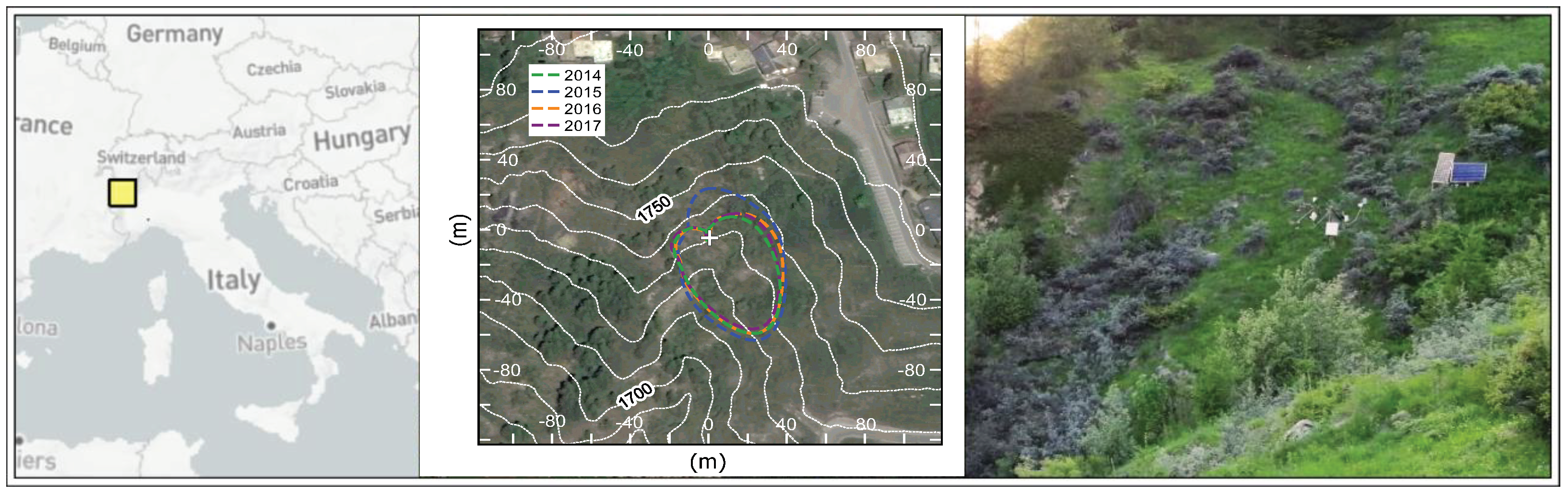
Table A1). Only one long-term EC site is located on an abandoned grassland in the Alps for eco-hydrological purposes, the Torgnon (IT-Tor) site [
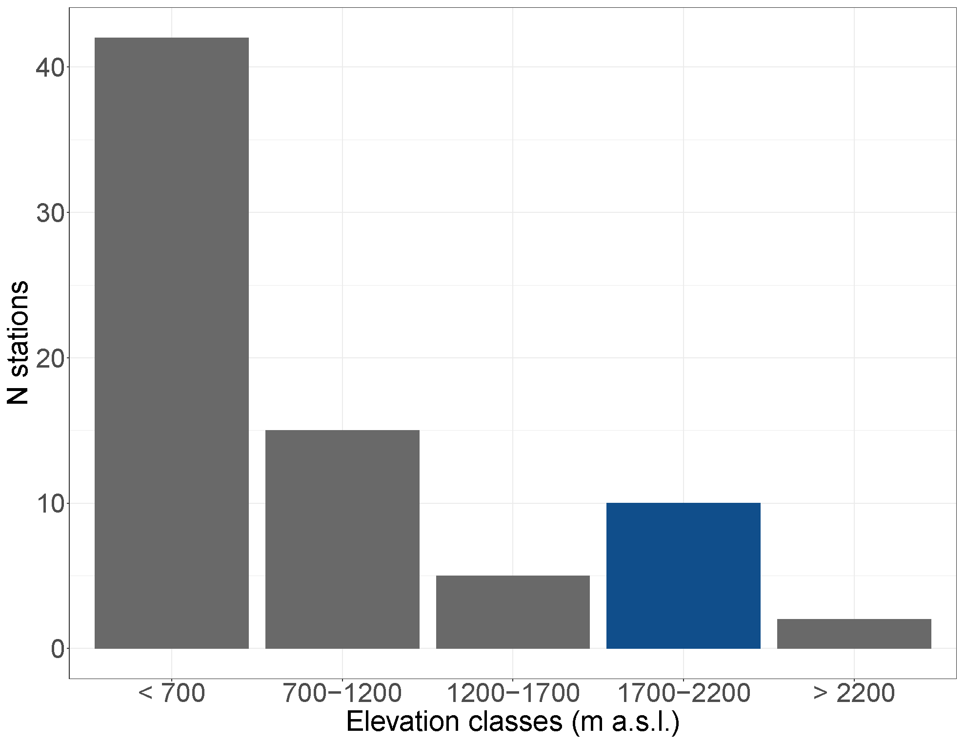
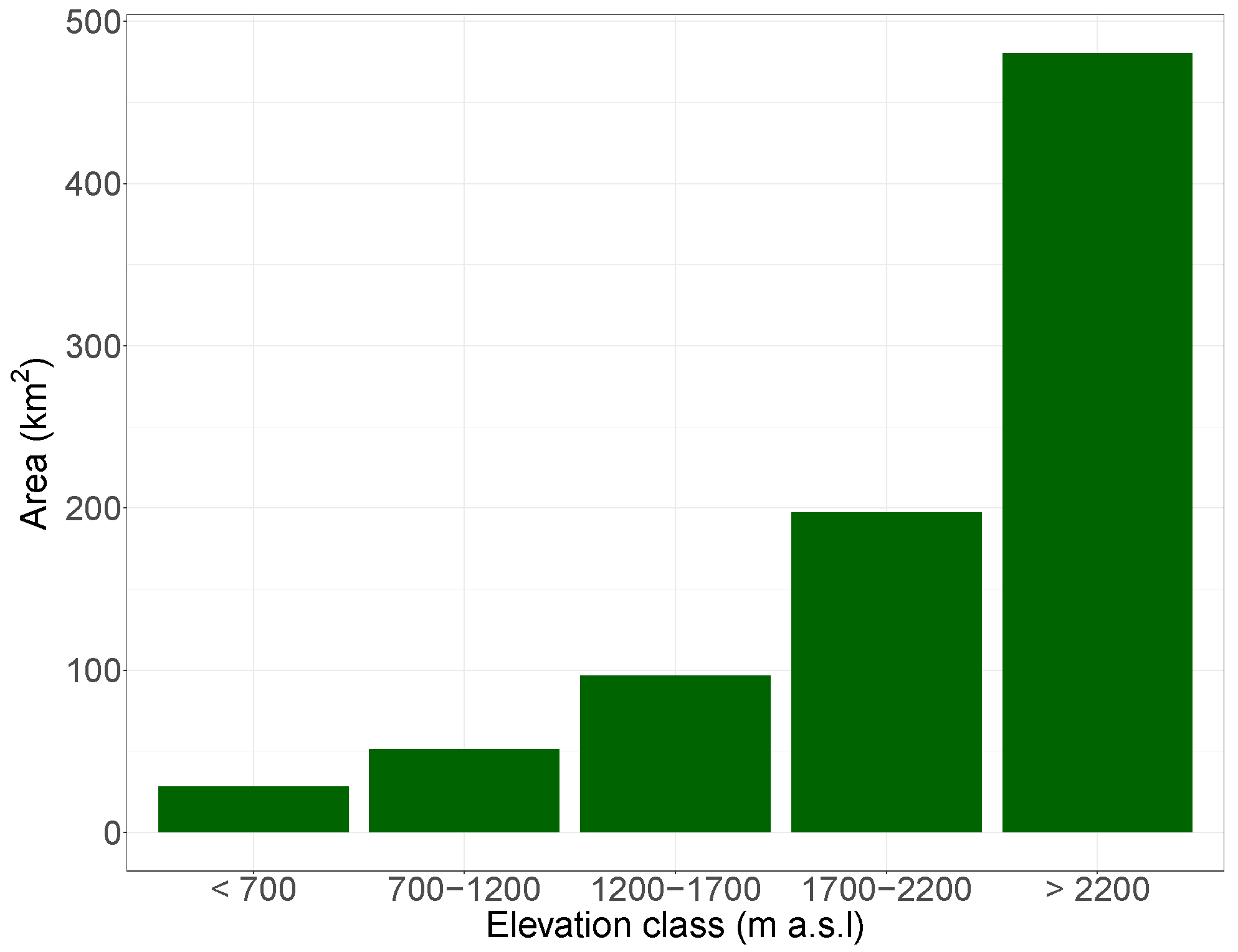
33] in Valle d’Aosta Region, in the Italian Western Alps. In that Region, grasslands cover up to 38% of the land surface area (1238 km 2 over 3260 km 2 , with the second highest portion of grassland cover between 1700 and 2200 m a.s.l., Figure A2 in Appendix A), and the topography can be very challenging. Besides, the Italian Western Alps are very interesting, since they are characterised by a wide range of altitudes within few kilometres, act as a powerful barrier against Atlantic perturbations, and close to a warm sea (the Mediterranean). The unique location could lead to enhanced meteorological intra- and inter-annual variability.
The Alpine environment is characterised by an enhanced topographical complexity. First, ETa complexity relies on its spatial variability, although not explored in the current study. One study aimed to correct ETa for elevation and slope [34], whereas [35] studied the spatial variability of ETa (and soil water content), but from a modelling point of view. Second, the measured fluxes (and ETa) are influenced by topography characteristics which affect the local meteorological conditions and measurements, such as valley system shape and orientation, analysed in the present study. These characteristics are important, as also illustrated by [36]. In the Alps, one of the first studies involving experimental data and numerical simulations was the RIVIERA project [37], where the turbulence structure and exchange processes in complex terrain were explored by means of experimental campaigns and numerical modelling. The influence of topography was made more clear, and [38], with a work on turbulence structure, post-processing choices, advection and surface energy balance understanding, found that the curvature of a valley alters the local wind circulation, and it significantly affects the fluxes (among which we find the latent heat flux). Besides, the need for exchange processes parameterisations in numerical weather prediction models was pointed out. Hence, the need for data is a consequent requirement. Turbulence structure and scalar-flux similarity were recently analysed, for turbulent fluxes, by [39,40]. In the Alpine Region, the only experimental setup that covers many years aiming at studying turbulence structure in the boundary layer, and air-land interactions at highly complex sites is the i-Box project in Austria ([12,41]). However, steep slopes with abandoned grasslands are still poorly explored.
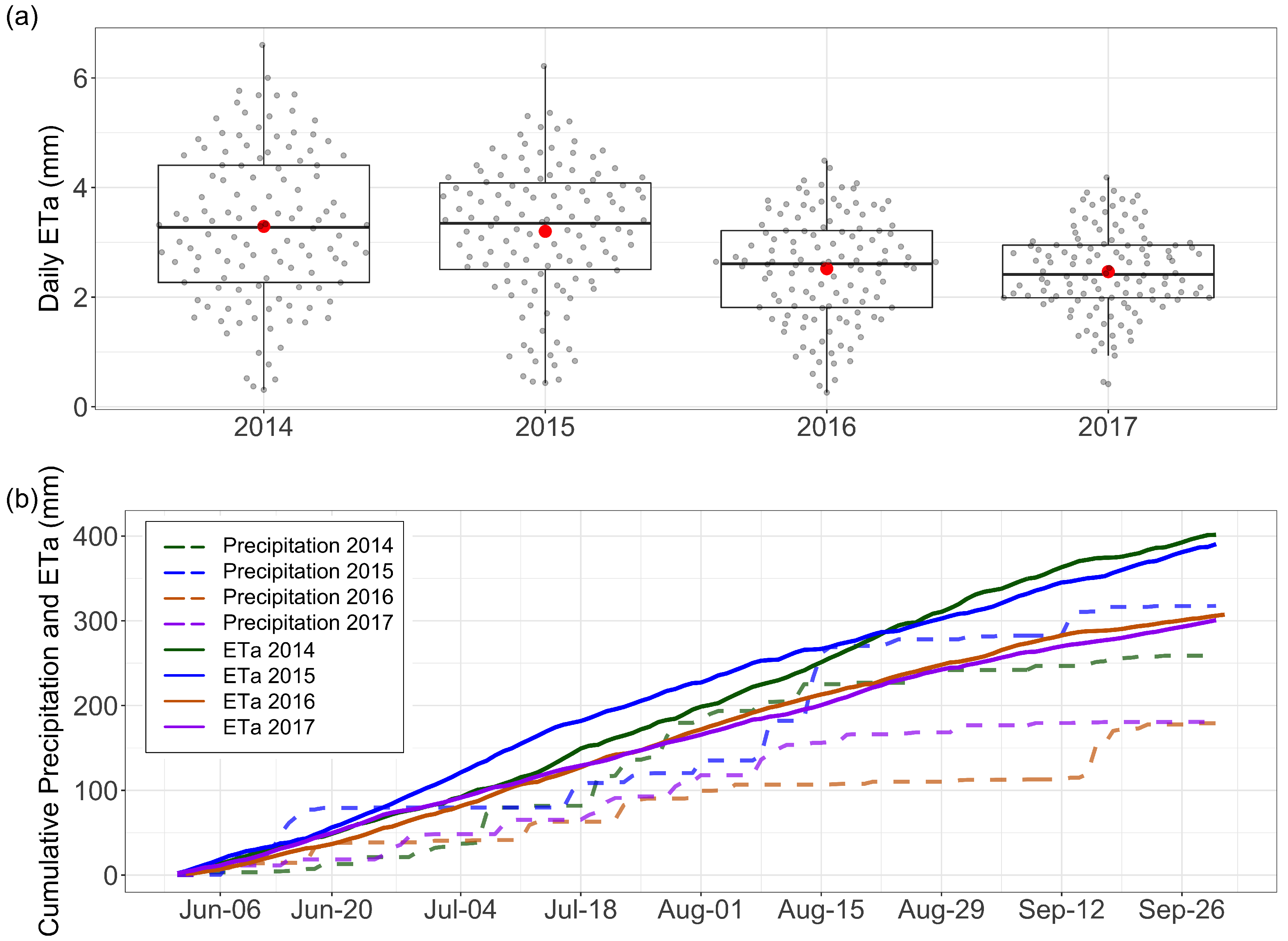
Considering different years, the varying meteorological and environmental conditions (warm/cold, wet/dry) can, with an analogy, represent different climate scenarios. However, especially the so-called inter-annual variability of meteorological and environmental variables, with a focus on ETa, is still subject to debate. Some studies did not find significant differences and also in limited-water years, the canopy did not experience water stress and ETa was not strongly water-limited [42,43]. Hence, a high meteorological variability might be required to observe differences among years and not all Alpine sites may experience it. Ref. [44] used EC data to measure ETa (and its inter-annual variability) and they found that ETa varies in response to precipitation. However, the study was not conducted in an Alpine environment. Ref. [45] characterised ETa over an unmanaged grassland and found that ETa inter-annual variation is due to annual precipitation differences. Both studies found enhanced variability for precipitation and ETa. Ref. [46] analysed shrubs (Eleagnus rhamnoides) and their impact on water availability due to their extended root system and competition with grass, with mature shrubs being able to extract water from shallow soil and also from groundwater when the water availability in shallow layers was reduced. Juvenile shrubs instead extracted water from shallower layers only. However, these behaviours may change across different growing seasons. Ref. [47] observed differences in ETa from sites having different land covers (cropland and grassland). Ref. [48] studied the ETa and water balance of a high-elevation, usually grazed grassland, and found ETa rates comparable with temperate Alpine areas. They also found that precipitation patterns significantly altered the canopy response.
Studies on ETa environmental drivers highlight the possible mechanisms on which the ETa relies. ETa depends on both environmental factors (solar radiation, air temperature, vapour pressure deficit, soil water content) and biological processes (leaf development, stomatal conductance, roots depth) as illustrated by [49]. Ref. [50] studied the ETa drivers also by means of eddy covariance, finding net radiation and VPD as the most important drivers, but they did not operate on Alpine ecosystems. According to [42], the most important drivers of ETa at an Alpine grassland in Austria were photosynthetic active radiation (PAR), R n (net radiation, strongly correlated to PAR) and VPD. Data from multiple stations in different ecosystems (but on Kilimanjaro mountain) were used by [51] to study the variables controlling ETa. In that study, R n , G (ground heat flux), VPD and precipitation were considered important ETa drivers (explaining also a high fraction of variance), and that land cover ETa dynamics and drivers might be obtained from short term measurements using very different ecosystems. Relative humidity and sunshine duration (two variables strongly correlated with VPD and both global and net radiation) explained most of data variance according to [52].
There is still a lack of knowledge about micrometeorological characterisation of a steep slope in a narrow valley with an abandoned grassland encroached by shrubs, an increasingly common ecosystem in the Alps, fastly expanding on slopes. In particular, an in-depth analysis focused on a hydrologically important variable, the actual evapotranspiration measured by the eddy covariance technique, is missing. The objectives of this paper are: 1. to evaluate the impact of local topography on ETa and other environmental variables in different growing seasons; 2. to quantify micrometeorological intra- and inter-annual variability of ETa and other environmental variables; 3. to identify the environmental drivers of ETa and how their impact changes across different growing seasons. This study will investigate these three themes with four growing seasons at an experimental site on an abandoned slope in the Western Italian Alps.

2. Materials and Methods

2.1. Site Description

The measurement site (Figure 1) is located in Cogne, Valle d’Aosta, Italy (45.615 N, 7.3585 E, 1730 m a.s.l.). The site is on a 200 m long slope of about 26° in a small lateral valley with South-East aspect. The site is characterised by high incident solar radiation due to its topographic orientation. This results in large daily air temperature variations. The climate is continental, with cold winters and hot summers. In the period 1995–2019, the average yearly precipitation was 672 mm, and the average temperature was 5.3 °C. During the growing seasons (i.e., from June to September) in the same period, the mean temperature was 12.5 °C, whereas the average precipitation was 230 mm.
The vegetation is characterised by herbaceous species (mostly Festuca, with a canopy height of about 0.3 m maximum) and shrubs (buckthorn bushes, Lycium, Eleagnus rhamnoides, with a typical height ranging from 0.8 m to 1 m). This vegetation is typical for abandoned grasslands, encroached by shrubs, at medium-high altitudes, making this site representative for many areas in the Alps. The soil depth ranges from 0.4 to 1.5 m and the soil consists of a sandy loam texture with some gravel (73% sand, 22% loam and about 5% of clay). The measured soil bulk density is 1.4 × 10 3 kg m 3 . The experimental site is located on an unmanaged grassland, next to a very small creek (East of the station) and no irrigation has been done for at least forty years. The other continuously operating EC site in Valle d’Aosta (Torgnon, IT-Tor, Fluxnet network) has different topographic characteristics, a different vegetation and no shrubs.
At the Cogne EC site, the wind is channelled, since it is characterised by an up/downslope regime with negligible mesoscale and cross-wind contaminations. Hence, very likely, the measured fluxes come mainly from the surrounding areas without other significant contributions. At the Regional Authority (ARPA-VdA) standard site, located 150 m West of the EC station, instead, the contributions from the main valley are important. The location choice in a complex area, hence, plays an important role for EC measures. (Figure A4 in Appendix A). The wind rose structure at the EC site in the analysed growing seasons is almost the same between different years.

2.2. Instrumentation

The EC station was equipped with the following instrumentation measuring at 10 Hz: a three-dimensional sonic anemometer (CSAT3, Campbell Scientific, Logan, UT, USA), and an open path infrared gas analyser (LI-7500A, LI-COR, Lincoln, NE, USA). The instruments were installed at 2 m above the surface and parallel to the slope. The 10 Hz measurements were averaged over 30 min periods. Non-eddy covariance instruments included sensors sampling every 30 min, and sensors sampling every minute with measures averaged at the 30-min scale. The first type of sensors included: 1. Three soil moisture probes (CS616, Campbell Scientific, Logan, UT, USA) at 10 cm—in 2014—and at 20 and 40 cm (from 2015) of depth. 2. Two thermocouples at 8 cm of depth (TCAV, Campbell Scientific, Logan, UT, USA). 3. One snow depth sensor (SR50AT, Campbell Scientific, Logan, UT, USA). The second type of sensors included: 1. Two probes installed at 8 cm of depth (HFP01SC, Hukseflux Thermal Sensors, Delft, The Netherlands) for the measurement of conductive soil heat flux (G). 2. One infrared surface temperature sensor (IRTS-P, Apogee Instruments, Logan, UT, USA). 3. One four-component radiometer (NR01, Hukseflux, Logan, UT, USA) to measure incoming and outgoing solar radiation and longwave radiation. 4. One thermohygrometer (HMP45C, Vaisala, Vantaa, Finland) replaced in January 2015 by a HMP155A (Vaisala, Vantaa, Finland).
The hourly precipitation measurements collected by a heated rain gauge were used in this study for the period 1 June–30 September in 2014, 2015, 2016 and 2017. The precipitation was collected at the Regional Authority (ARPA-VdA) station mentioned in Section 2.1. For the analysis, the EC data of four growing seasons (1 June–30 September, also called JJAS period, in 2014, 2015, 2016 and 2017) were used. For further meteorological and hydrological analyses, a hourly data set of precipitation was used, starting from 1 October 2013 to 30 September 2017. An extended data set, with both air temperature and precipitation from the ARPA-VdA station, was used for growing seasons from 1995 to 2019 to analyse possible historical trends of the two variables.

2.3. Data Processing, Quality Control and Analysis

2.3.1. Eddy Covariance and Radiation Fluxes

The EC data were processed using EddyPro 6.2.1 software (LI-COR Biogeosciences, Lincoln, NE, USA). The obtained EC data set contained half-hourly data. To compute the sensible (H) and latent heat ( L E ) fluxes, corrections were applied: linear detrending and double rotation [8], high and low-pass filtering corrections ([17,53]), Webb-Pearman-Leuning (WPL) correction for air density fluctuations [54], humidity correction of sonic temperature [55] and time lag detection and compensation by covariance maximisation [56]. Depending on the wind flow direction, the canopy height changed. When wind came from the sectors 0–90° and 270°–360°, h c a n o p y = 1 m. For the other sectors, h c a n o p y was measured by the snow depth sensor, which in summer measures the grass height. The roughness length was then estimated as z r = 0.15 · h c a n o p y . This empirical choice, also used by EddyPro software, gave reliable values if compared to those found in many micrometeorology books (e.g., [8]).
Spikes were removed on 10 Hz data time series using the algorithm described by [15]. Statistical tests based on [20] were firstly performed on single variables recorded by the sonic anemometer and gas analyser: check for unphysical values (Table A2 in Appendix A); skewness and kurtosis; drop-outs and discontinuities. For each half-hour, fluxes were discarded if at least one of the variables used to compute fluxes was hard-flagged (i.e., it was considered of low quality). The covariances used to compute turbulent fluxes ( w T ¯ and w H 2 O ¯ ) need to satisfy the steady-state and integral turbulence characteristics. This test was assessed using the 0-1-2 flagging scheme reported in the TK3 software package [25] (0: reliable data; 1: intermediate quality data; 2: bad quality data). Furthermore, the flux uncertainty was estimated as in [12]. Half-hour periods with an error on covariances greater than 50% were also hard-flagged. This threshold was chosen since in complex terrain the uncertainty is usually larger than at homogeneous sites [12]. The half-hours with precipitation were also hard-flagged. For each half-hour period, an overall flagging code was obtained combining all the previous controls on data, and the gas analyser gain control in a single flag (0 = good quality; 1 = bad quality). A control on unphysical values of net, global and shortwave radiation was also implemented. Then, the daytime data were identified using global radiation measurements and a cross-check with local sunrise and sunset, setting a threshold of 10 W m 2 as in [57]. EC nighttime data were discarded because most of the evapotranspiration occurs during daytime hours.

2.3.2. Soil Variables and Surface Energy Balance

The volumetric soil water content, measured at 10, 20 and 40 cm of depth was checked for unphysical values. At the daily scale, missing data were linearly interpolated. The shallow soil water content, hereafter also called shallow θ , was the soil water content between 10 and 20 cm. The volumetric soil water content measured at the three depths was also converted into equivalent millimetres weighting it by the soil depth above the sensors. To maintain the best coherence possible between 2014 and the following years, the 10 cm (from 2014) and 20 cm depth (2015–2017) soil water content were mainly used for inter-annual comparisons. The wilting point and the field capacity soil moisture values were estimated by means of water retention van Genuchten curve [58], with parameters extracted from [59]. The obtained values were 0.024 m 3 m 3 for wilting point and 0.149 m 3 m 3 for field capacity. These values are reasonable, also according to the Cogne site properties found by [60].
The 30-minute ground heat flux was measured, and the soil heat storage flux above the soil heat flux sensors was estimated as in Equation (1), [61]:
S s o i l ( t ) = Δ T s o i l · C s o i l · d Δ t ,
where Δ T s o i l is the measured soil temperature variation in time at each time step, C s o i l (J kg 1 K 1 ) is the soil heat capacity, d (m) is the soil depth at the site and Δ t is the time step (here 1800 s). The soil heat capacity was estimated as in [62]. The canopy heat storage flux was also included and estimated as in [16] (Equation (2)).
S c a n o p y ( t ) = Δ T s u r f a c e ( C w · m w + C o · m o ) Δ t ,
where Δ T s u r f a c e / Δ t is the rate of change of measured surface infrared temperature, C w = 4190 J kg 1 K 1 is the water heat capacity, m w = 0.38 kg m 2 is the above-ground organic water mass and m o = 0.30 kg m 2 is the above-ground dry organic mass. C o = 1920 J kg K 1 is the dry organic heat capacity. The overall storage term was then estimated as S = S s o i l + S c a n o p y . Nighttime data of soil heat fluxes were discarded (as done for EC data). To complete the data set, the water vapour pressure (e) was computed using the relative humidity measurements from the thermohygrometer and the saturation vapour pressure ( e s ) computed as suggested by [63]. The vapour pressure deficit (VPD) was also computed as e s e .
The net energy balance (Equation (3)) was investigated through the RMA (ranged major axis) linear regression for each growing season using the lmodel2 R package [64].
H + L E = R n G S
where H and L E are, respectively, the sensible and latent heat flux, R n is the net radiation, G is the ground heat flux (at 8 cm of depth) and S is the overall soil storage term above the ground heat flux sensor. More than 70% of data was considered reliable during daytime (i.e., roughly between 7:00 and 17:00) after the data quality control. The quality of turbulent fluxes decreased around sunrise and sunset (Figure A3). These findings were in agreement with [11,12,14]. The energy balance closure ranged between 60% and 70% (Table 1). The energy balance closure found at the research site confirmed a still open issue about EC measurements on complex terrains, but the closure was within the range of previous findings. Ref. [11] described a balance closure with a slope of the regression line of around 70%; Ref. [14] found a closure of around 80% for a relatively small data set; Ref. [65] found a range oscillating from 55 to more than 90%.
Being aware of the possible underestimation of turbulent fluxes with EC, the Bowen ratio correction (e.g., [66,67]) was also tested. However, the resulting ETa (Section 3.2.2) was suspected of being unrealistically high, especially if compared to the measured precipitation between June and September, but also on the whole hydrological year. The ETa corrected using the Bowen ratio ranged from 68 to 77% of the annual precipitation in just four months. It was preferred to keep the purely measured eddy covariance ETa because the current study was neither focused on surface energy balance nor on hydrological balance. Furthermore, the Bowen ratio correction adds uncertainty related to the necessary additional hypotheses adopted when corrected fluxes are computed (e.g., [66]). Also, the Bowen ratio correction may affect the results of ETa drivers investigation, because the corrected L E flux is strongly related to the terms R n (net radiation) and G 0 (ground heat flux at the surface).

2.3.3. Eddy Fluxes Gapfilling and Flux Footprint Estimate

The latent and sensible heat fluxes were gap filled using the ReddyProc R package [68]. The mean diurnal sampling (MDS) algorithm was used as in [69]. The ETa was computed dividing L E by the latent heat of vaporisation of water. The quality-controlled gap filled data set was then aggregated at the hourly and daily scales. Gaps in other time series (solar radiation, net radiation, and ground heat flux) were uncommon. They were not filled at the half-hourly or hourly scales. At the daily scale, days with few or missing data were linearly interpolated.
The flux footprint was evaluated for each growing season using the model implemented and described by [70]. The boundary layer height was estimated using ERA5 reanalysis [71] hourly data on the 0.25° × 0.25° grid cell nearest to the site. Footprints of the site in the four growing seasons are shown in Figure 1. The footprint was almost constant throughout the years (Figure 1). This made the inter-annual comparison more robust. Besides, the footprint was rather small and homogeneous, reaching about 40 m from the station along the main wind direction.

2.3.4. Statistical Methods

The inter-annual differences of meteorological and soil variables were also assessed using a two-sided t-test included in the “stats” R-package [72]. There are several ETa drivers, on which meteorological conditions temporal variability might play a role. As a first approximation, and to understand the contribution of each variable to ETa at the daily scale, a linear combination of net radiation ( R n ), vapour pressure deficit (VPD), ground heat flux at the surface ( G 0 ), wind speed (U) and air temperature ( T a i r ) was used to obtain ETa (Equation (4)). The wind speed was included because the variable is considered in some potential evapotranspiration formula, and because the ETa was estimated via EC technique. In this linear model, the soil water content and the precipitation were not included because of non-trivial relationships and time lags (more than one day) due to soil processes dynamics and, for soil water content, because only shallow measures were available (possible time lags). Soil water content (shallow θ at maximum 20 cm of depth, if not otherwise specified) and precipitation (P) were analysed separately. Periods of 15, 26, 35 and 52 days were considered. Instead, the ETa drivers in the linear model were explored at the daily scale.
E T a = a 1 R n + a 2 V P D + a 3 G 0 + a 4 U + a 5 T a i r ,
where the coefficients a n are the regression coefficients.
Prior to the regressions, the variance inflation factor (VIF) was computed to identify possible collinearities among the possible drivers of ETa. Results highlighted that VIF < 6.7. Up to 10, usually the multicollinearity can be considered low [73]. Hence, as a first approximation, a linear model could be used. A linear mixed model was assumed to identify the contribution of random effects (variability between different years, grouping data according to the variable “year”) and of fixed effects (the five drivers enumerated earlier), using “lme4” R package [74]. The R 2 values of fixed effects (marginal R 2 ) and of the fixed and random effects (conditional R 2 ) were computed following [75] and using the “MuMIn” R package [76].
A multivariate analysis can help identifying the most important drivers contributing to ETa. The multivariate analysis was performed on the four growing seasons together and in each growing season. To assess the importance of drivers, a stepwise multiple linear regression can be used, as in [42,50]. The approach followed in the current paper was based on the minimisation of Akaike information criterion (AIC) [77]. The lower the AIC, the better the model. The stepwise regression was computed using the “MASS” R Package using only complete cases (i.e., when all the variables were available) [78]. When the number of samples was low if compared to the number of parameters (i.e., in single growing seasons), the AIC corrected for finite sample size (AICc, [79]) was used for the stepwise regression. The minimisation of AIC (or of AICc) led to the identification of the most important drivers. The fraction of variance explained by the drivers was instead assessed using the adjusted R 2 coefficient. To better understand the role of each separate driver—namely, R n , VPD, G 0 , U and T a i r and to quantify the degree of variance explained by each of the separate drivers, they were analysed separately with univariate regressions (considering all growing seasons together and single growing seasons). In the univariate regressions, the natural logarithm of VPD was identified as a better driver of ETa, in agreement with [42].

3. Results

3.1. Topography Influence on Actual Evapotranspiration and Its Inter-Annual Variability

3.1.1. Wind Regime and Latent Heat Flux Sources

An evident difference between daytime and nighttime wind regimes was identified, with daytime flow coming mainly from South-South East (upslope wind) and a North-coming (downslope) wind regime during nighttime (Figure 2, left panels for each growing season). This regime was observed in all the four growing seasons. The low-wind speed conditions (LWS, wind speed lower than 1.5 m s 1 [80]) prevailed in all the growing seasons (Figure 2, right panels for each growing season), and, overall, more than 80% of hours were characterised by LWS conditions. The daytime upslope flow was on average characterised by a higher wind speed due to thermal pumping. The colour maps allow to localise the possible sources and sinks of water vapour.
The main source of water vapour was located to the South-East of the station (Figure 2a,b), where a moist area with some shrubs exists. To the South-West and West of the station instead a drier area was found. This area has been also colonised by shrubs. Most of potential sources of water vapour and of latent heat during wet growing seasons were less active or non-existent in dry growing seasons (Figure 2c,d). This suggested that the small creek within the small valley had negligible effect on fluxes because the water discharge was constant throughout the four growing seasons.

3.1.2. Morning Latent Heat Flux Inflexion and Mean Diurnal Cycles of Fluxes

At the sunrise, L E (and H) increased greatly and rapidly. A sharp decrease occurred at the sunset, in particular for R n , because of mountain shadowing (Figure 3). A morning inflexion (i.e., a change in the diurnal course slope) was visible for all the growing seasons for air temperature, L E flux (Figure 3), H flux, RH and VPD (Figure A5, Appendix A). The same phenomenon was also visible for a limited number of days and on single days (Figure 4). The inflexion was instead not found for net radiation (Figure A5, Appendix A). The inflexion was always found near the hours in which the transition from nocturnal to diurnal wind circulation occurred (i.e., from downslope to upslope, between 7:00 and 9:00, as shown by wind direction in Figure 3 and Figure 4).
The L E flux mean diurnal cycle in wet growing seasons showed higher values than in dry growing seasons (Figure 3a,b compared with Figure 3c,d), with differences up to about 100 W m 2 in the hours between 08:00 and 15:00. The L E range between ±1 σ was always near 100 W m 2 ( 80 W m 2 in 2017 and 130 W m 2 in 2015, Figure 3a,b). The air temperature difference between 2014 and the other growing seasons was also visible in its mean diurnal cycle. In 2014, the mean air temperature was about 2 °C lower than in other growing seasons around midday, and the net radiation had the second highest variability after L E (up to around 70 W m 2 , Figure 3), with 2014 being the year with lowest values due to frequent cloudy days and precipitation events. For H (Figure A5, Appendix A), the inter-annual differences in the hours 08:00–15:00 of the day were lower if compared to L E (no more than 42 W m 2 ), and the cycle variability (±1 σ ) was lower than the one found for L E (maximum 70.7 W m 2 in 2016 growing season).

3.2. Micrometeorological Intra- and Inter-Annual Variability

3.2.1. Meteo-Climatic Variability at the Experimental Site

Over 25 years (1995–2019), the mean air temperature of June-September period varied between almost 11 °C (1995–1996) and 15 °C (2003). A positive trend of 0.07 °C year 1 was found (significant, p-value < 0.05). The 2014 growing season showed one of the lowest average temperatures of the 2009–2019 decade, whereas the other three years were closer to the regression line (Figure 5a). The precipitation (Figure 5b) did not show any significant trend, but the four considered growing seasons (2014–2017) showed a relatively high precipitation variation.
Considering only the four selected growing seasons, the wettest growing season was identified in 2014, as illustrated by the combination of higher RH, precipitation and its timing, and lower average dry spell (a dry spell was defined according to [82]). Overall wet conditions emerged also in 2015 (Table 2). The high average and maximum dry spell found in 2015 (due to a dry period between June and July) did not cause particular effects on the growing season because of higher precipitation and higher precipitation frequency compared to 2016 and higher precipitation if compared to 2017. The 2017 growing season experienced frequent precipitation grouped during contiguous days, but, if compared to 2014, less sparse events with more dry days between events and with lower precipitation, especially in the middle growing season. The average dry spell in the period May–June (the precipitation occurred in May has deep influence on JJAS ETa) was comparable with that of the 25 years average (5.1 ± 4.6 days, considering May-September periods). Also, the maximum dry spell in 2015 (28 days between June and July) was found earlier, between May and June 1996 (29 days). Between 2014 and 2017 growing seasons, the precipitation difference reached up to 100 mm for both the hydrological year and the growing season. Differences of more than 60 mm occurred in the sole month of May (2016 experienced the highest cumulative precipitation in May).
Differences of mean air temperature in the four analysed growing seasons were always greater than 1 °C between 2014 and the other growing seasons (up to 1.4 °C between 2014 and 2016). Within the identified growing seasons different scenarios of growing season existed. These scenarios were useful to illustrate the ecosystem behaviour with an environment having different average temperatures. The inter-annual variability of L E (hence, ETa) was also evident from the L E / R n ratio. L E covered a much higher portion of available energy (net radiation) in wet growing seasons than in dry ones (Table 3).
Summarising, an inter-annual variability of several variables (air temperature, precipitation, dry spell length, relative humidity—RH, L E / R n ) was found.

3.2.2. Average Daily and Cumulative Actual Evapotranspiration in the Growing Seasons

The daily ETa averages and cumulative ETa over the growing seasons identified intra- and inter-annual patterns. In wet growing seasons, the intra-annual ETa standard deviation was higher if compared to dry ones. Moreover, in wet growing seasons, ETa daily averages showed enhancements of about 0.8 mm day 1 (Figure 6a). The cumulative ETa also showed an enhanced inter-annual variability, especially between the driest (2016) and the wettest (2014) growing seasons. Besides, both ETa and P showed cumulative values differences of more than 100 mm (Figure 6b), with an evident gap between dry and wet growing seasons. The aforementioned values considering Bowen ratio correction of L E were 535 mm, 513.8 mm, 454.1 mm and 458.1 mm, respectively in 2014, 2015, 2016 and 2017, hence showing an enhancement if compared to the uncorrected ETa. The inter-annual differences did not change severely. The ETa in 2014 was the highest (despite relatively low air temperature and high RH) for several reasons: 1. frequent precipitation events (average dry spell: 4.2 days) which compensated a lower precipitation if compared to 2015; 2. a sufficient precipitation during the hydrological year and also during the growing season; 3. optimal timing of precipitation, mainly occurring in the middle of the growing season, when the vegetation is fully active; 4. high water availability.
Between 2015 and the following two growing seasons in 2016 and 2017, the average air temperature differences were very low (around 0.1 °C). However, the ETa deficit was greater than 60 mm (60.7 mm and 75.4 mm, respectively). The low ETa in 2016 was explained by a combination of a relatively long average dry spell (5.5 days), only 18 days with precipitation and low cumulative precipitation of 179 mm. The low ETa in 2017 was explained mainly by low precipitation (also in May), low soil water content, high air temperature and an average dry spell (6.1 days) close to the other dry growing season. Instead, the number of rainy days (29 days) was comparable to the ones found in the 2014 wet growing season. The 2016 growing season experienced higher cumulative ETa than in 2017 because of precipitation events in August.

3.2.3. Bimodality of Environmental Variables

L E (hence, ETa) and other environmental variables showed a bimodality of frequency density distributions (Figure 7a). For L E , the bimodal distributions showed one peak around 20 W m 2 and the other between 100 and 250 W m 2 . The L E bimodality might be related to two distinct regimes: the first occurred during daytime transition hours, near sunrise and sunset (i.e., 5:00–8:00 and 17:00–20:00, light red histogram), when L E release occurred, but the values were low because of low radiation forcing. The second regime occurred when the photosynthesis of vegetation and, hence, ETa, were no more inhibited (between 8:00 and 17:00, grey histogram, when the wind flow and L E came from South along the slope—i.e., with upslope wind regime—and the radiation forcing was high). Dry growing seasons showed a more evident second peak if compared to wet ones. The bimodality explanation was confirmed by the frequency density distribution of net radiation, which, however, did not show significant differences between mean values in different growing seasons (Figure 7b).
In addition to L E and R n , shallow volumetric soil water content ( θ , between 10 and 20 cm of depth, Figure 7c) showed a bimodality, particularly evident only in 2015. This can be explained by the presence of one prolonged dry period between June and July (DOY 185–223, light red histogram in Figure 7d) and two wet periods (DOY 164–184 and 224–253, grey and green histograms, Figure 7c). A bimodality was also found for ground heat flux at the surface ( G 0 , Figure 7d), driven by R n . Similarly, the bimodality of U (Figure A6a) was distinguishable, which can be explained by the two wind regimes, one during daytime (upslope, with higher wind speed) and one during nighttime (downslope). VPD and T a i r distributions did not show any particular bimodality (Figure A6b,c).
Finally, a statistically significant difference (p-value < 0.05) between the mean L E and shallow θ distributions in wet and dry growing seasons was found. In addition, significant differences (but with higher p-value still lower than 0.05) were also found between seasons in similar water availability conditions, with the exception of 2014 and 2015 average shallow θ .

3.2.4. Evaporative Fraction, Soil Water Content and Evapotranspiration Regimes

Two approaches were used to assess energy-limited and water-limited conditions. The first was the relationship between evaporative fraction (EF) and soil water content ( θ , at 10–20 cm, Figure 8). The soil water content at 40 cm of depth was also used to test the relationship with EF (not shown). The second was the comparison between ETa and potential evapotranspiration ETo (Figure 9).
An EF increase with increasing shallow θ below 0.07 m 3 m 3 was noticed. The trend was less clear for shallow θ values greater than 0.075 m 3 m 3 , with scattered data. Besides, decreases of EF were found between 0.075 m 3 m 3 and the field capacity (0.149 m 3 m 3 ), not reached in 2017. A possible critical shallow θ was slightly higher than 0.05 m 3 m 3 . However, a dramatic decrease in EF below that point was not observed. An EF increase with soil water content was observed only in 2014 (one of the wet growing seasons). On the opposite, in the 2015 and 2016 growing seasons, an oscillating trend was found. In 2017, an increase below 0.075 m 3 m 3 was found, followed by a decrease for higher θ values. Using the 40 cm soil water content, the results did not change dramatically (not shown). It should however be pointed out that a relatively superficial soil water content (down to maximum 40 cm of depth) was available. The behaviour of daily average of EF (using only the hours in the range 8:00–15:00) was similar to the EF value extracted at local solar midday (12:00) (Figure 8a,b) in all growing seasons. Differently from theoretical behaviours, using both EF computations, the identification of water and energy-limited regimes was not trivial.
The ETa regime was better identified using the potential evapotranspiration (ETo), estimated via Penman-Monteith equation [84]. The energy-limited conditions were more evident in 2014, when the soil water content at 10 cm of depth was relatively high and the ETa was closer to ETo, if compared to the remaining three growing seasons. In those growing seasons, water-limited conditions were more frequent (Figure 9). The water limitation was evident already in 2015, and mostly in 2016 and 2017. In 2015, the dry period between June and July was also noticeable from the low soil water content at 20 and 40 cm of depth. That period caused a decrease in ETa (consistently lower than ETo). Higher (up to more than 4 mm day 1 ) discrepancies between ETa and ETo occurred in water-limited growing seasons (2016 and 2017), when the soil water content decreased to less than 20 equivalent millimetres stored in the soil layers, at 20 or 40 cm of depth.
The ETa response to precipitation is shown in Figure 9. In all growing seasons, when precipitation occurred, the ETa was reduced and then slightly increased the following days. However, this increase was not always observed, because of lower air temperature and VPD (as at the beginning of August 2016) and/or still lower water availability (Figure 10). Despite these results, a significant daily correlation between ETa and both precipitation and soil water content was not found because, as explained in Section 2.3.4, there are time lags (greater than one day) between these two variables and ETa.

3.2.5. Fifteen-Days Analysis of Micrometeorological Variables

The intra- and inter-annual variabilities of micrometeorological variables were more deeply analysed considering periods of 15 days (Figure 10). The intra-annual variability included a T a i r , VPD, and EF decrease in late growing seasons. The precipitation largest peaks were usually found in the middle of the growing seasons, with some exception in 2015 and 2016. The cumulative ETa showed a clear bell-shaped trend (with the peaks found in the middle of the growing season) in 2014 and 2016, differently from the other two growing seasons. In 2015, the different behaviour was likely due to the long dry period between June and July, whereas in 2017 the precipitation scarcity played an important role.
The inter-annual variability emerged in the following findings. The lowest T a i r values were found in 2014 in most of the 15-days periods. Variations of more than 5 °C were identified in 15-days periods in different years (Figure 10a). The VPD (Figure 10b) was lower in 2014 by more than 1000 Pa in the period 1–15 July, if compared to 2015. Year 2015 showed enhanced VPD due to the wide period with high air temperature and without precipitation, as also illustrated in Figure 10c,d, where the average precipitation per day and number of dry days are shown, respectively. An important decrease in average EF (Figure 10e) and cumulative ETa (Figure 10f) was noticed in the same—but drier—periods of years 2016 and 2017 if compared to wetter years 2014 and 2015, because of lower water availability and despite a high VPD. During the long dry spell of 2015 (June–July), and especially in the first decade of July, T a i r and VPD were sufficiently high to cause a peak of EF (and ETa), despite relatively low water availability. In addition, periods with wet conditions (e.g., 30 June–15 July 2014) could experience high EF and ETa, even with relatively low T a i r and VPD. The major EF difference (0.2) was found in the two 15-days periods of September 2016 and 2017 if compared to the other two growing seasons. This finding was coherent with ETa, which showed reductions of about 10 mm in the same aforementioned periods. ETa inter-annual differences could be greater than 15 mm, and the highest EF and cumulative ETa were found in 2014 in 4 out of 8 periods.
In summary, inter-annual differences existed in most of 15-days periods for all the variables. The 15-days analysis better identified the causes of 2014 being the year with the wettest growing season. Despite an overall higher precipitation in 2015 if compared to 2014, in 2014 a high precipitation occurred earlier. Besides, a higher precipitation frequency occurred in the growing season with two important peaks in early July. Years 2014 and 2015 experienced the highest precipitation in the early-to-middle growing season, providing water when the vegetation was more active. The EF and ETa showed similar intra- and inter-annual trends, and showed higher values during days with high VPD and T a i r .

3.3. Evapotranspiration Environmental Drivers

ETa is governed by vegetation strategies, but also by several environmental drivers. The most important drivers include variables previously analysed such as R n , VPD, U, G 0 and T a i r . Precipitation and soil water content are also important drivers, but, as described in Section 2.3.4, their relationship with ETa is not trivial and it was analysed separately in Section 3.3.3. The highest correlations existed between R n and G 0 (R = 0.88, both hourly and daily values) and between VPD and T a i r (R = 0.89 for hourly values and R = 0.74 for daily values). The mean diurnal cycles of VPD and T a i r highlighted also inter-annual differences, with T a i r in 2014 growing season being lower than in other growing seasons. Consequently, sensibly lower VPD was also found (Figure 11).

3.3.1. Actual Evapotranspiration Linear Mixed Effects Model and Multivariate Regressions with Environmental Drivers

Results from the linear mixed model highlighted a contribution of both random and fixed effects, since the marginal R 2 (related to fixed effects) was 0.56, whereas the conditional R 2 (related to the fraction of variance explained by both the fixed and random effects) was 0.83. The inter-annual variability itself played a key role in changing ETa from one growing season to another, because the role of random effects was not negligible. Among the five drivers, the most important were R n , U and VPD, as indicated by AIC and p-values in Table 4 and by the stepwise minimisation of AIC. The removal of G 0 and T a i r did not imply a high loss of information, since they were eliminated by the stepwise process. This result was confirmed also looking at the adjusted R 2 which did not change appreciably if G 0 and T a i r were removed from the model.
The importance of the drivers changed inter-annually (Table A3, daily set of data for each growing season). The stepwise multivariate regressions showed, in agreement with the p-values shown in Table A3, that R n , VPD and U could be included in every simplified linear model of ETa, as indicated by AICc minimisation algorithm and by AICc and p-values of Table A3. Hence, they could be considered the most important drivers except in 2017, when VPD was replaced by G 0 . In 2014, the stepwise AICc minimisation suggested to remove G 0 and T a i r . In 2015, T a i r could be included, while G 0 was not significant. In 2016 T a i r was replaced by G 0 , whereas in 2017 no variable was excluded. The complete model included all the analysed drivers and was used, for coherence, in every year subset. The model showed a relatively large variability of the explained variance, between 0.67 and 0.87 (Table 5).

3.3.2. Actual Evapotranspiration Univariate Regressions with Environmental Drivers

The highest fraction of explained ETa variance was given, for the entire data set of four growing seasons, by R n , G 0 and VPD (Table 6). Considering each one of the four growing seasons separately, univariate regressions results are shown in Table 7. The most important ETa driver was VPD, followed by R n . R n , VPD and G 0 accounted for a reduced explained variance in the wettest and coldest growing season (2014). Moister air and less frequent sunny conditions may explain the lower fraction of variance explained. U explained always the lowest variance, likely because the wind speed did not experience high values. T a i r explained a higher fraction of variance in the dry growing seasons.

3.3.3. Actual Evapotranspiration Relationship with Precipitation and Soil Water Content

The effect of precipitation and soil water content on ETa were analysed, and these showed not to be trivial. The two dry growing seasons showed clearly a different behaviour than the wet ones, since ETa data laid on different regions if plotted against cumulative P and average θ (Figure 12 and Figure A7, in Appendix A, for 15 and 52-days periods). ETa versus P showed very weak trends with R 2 values up to 0.15 considering 52-days periods (Figure A8a, all regressions are not significant). Considering the ETa versus θ relationship (Figure A8b, all regressions are not significant), the fitted data from 15, 26 and 35 days showed again trends close to zero, indicating no or little direct dependence on soil water content. Only the 52-days period ETa versus θ showed a clearly positive slope and a relatively higher R 2 of 0.45 (not significant, given the low number of data). Summarising, the results indicated no or little direct dependence on precipitation and soil water content (Figure A8 in Appendix A).

4. Discussion

4.1. Topography Influence on Actual Evapotranspiration and Its Inter-Annual Variability

The strongly bimodal wind flow regime, and in particular the wind direction shift in the morning from downslope to upslope (Figure 3 and Figure 4), played a key role in the measured fluxes and other micrometeorological variables. The wind flow was thermally driven as described by [85], and changed from downslope to upslope in the morning (between 7:00 and 9:00). Aloft with respect to the experimental site, visual observations and local shading allowed to suppose that solar radiation and R n , increased earlier than the wind shift occurrence. Hence, the wind speed carried heat from an area already illuminated. When wind, influenced by local topography, shifted from downslope to upslope, a colder air flow coming from the bottom of the valley carried latent (and sensible) heat from an area still cold. Moreover, this colder air caused a temporary inflexion of RH and, hence, of VPD. These wind circulation-induced effects affected L E (ETa) through air temperature and VPD, and might explain its inflexion. A similar inflexion was found by [38], where turbulence exchange mechanisms and boundary layer properties were explored in highly complex terrain.

4.2. Micrometeorological Intra-and Inter-Annual Variability

4.2.1. Meteo-Climatic Variability at the Experimental Site

In addition to the results described in Section 3.2.1, the meteo-climatic variability was also assessed using the L E / R n ratio. This ratio, at Cogne, varied between 41% (2016) and 58% (2014). The maximum value and also the variability range are comparable with the findings of [86] (62% and 42.2%, respectively the maximum and range variability values). An important reduction was found in dry growing seasons as also documented by [87]. The ETa reduction was also confirmed, at Cogne, by the inhibited sources in dry growing seasons (Figure 2).

4.2.2. Average Daily and Cumulative Actual Evapotranspiration in the Growing Seasons

The average ETa for the whole growing season was 3.3 and 3.2 mm day 1 in 2014 and 2015, whereas it was 2.5 mm day 1 in 2016 and 2017. Maximum values reached up to 6.6 mm day 1 in wet growing seasons (2014) and up to 4.5 mm day 1 in dry growing seasons (2016) as shown in Figure 6. The daily ETa range is comparable with the findings of [88] (Subalpine grassland) and [89] (Alpine grassland), which reached around 5.3 mm day 1 , and of [86] (up to 6.8 mm day 1 on an Alpine grassland during the growing season).
The cumulative precipitation inter-annual variability was also higher than 100 mm in contiguous years (Figure 6). This high variability of precipitation is much higher compared to around 40 mm of difference found in other studies ([42,86]). The cumulative actual evapotranspiration in the four growing seasons at the Cogne site (300 to 401 mm) is comparable with literature findings: Ref. [42] found values ranging from 250 to 450 mm but on an annual basis in the Austrian Alps; Ref. [88] found 350 mm in the JJAS period in a Subalpine grassland. In addition, the inter-annual ETa differences were within the range of variability of climate change-induced variations (up to around 100 mm) as simulated by [90] for the Alps with a +3 °C temperature increase scenario. However, in the current study lower inter-annual average T a i r differences were found (around maximum 1.5 °C).

4.2.3. Inter-Annual Variability of Actual Evapotranspiration and Precipitation: A Focus

A high inter-annual variability was also quantified with the coefficient of variation of ETa and precipitation P. The ETa coefficient of variation (CV) in the current study was 15.3%, compared to 7.1% found by [42], and the CV for P was 8.8%, compared to 18.6% found by [42]. In that study, the ecosystems were Alpine grasslands not encroached by shrubs. The growing season ETa ranged from 48.1% to 57.7% of hydrological year cumulative precipitation, respectively in 2017 and 2014. These findings suggested an enhanced inter-annual variability at the Cogne site compared to the Austrian one.
In warm growing seasons, the ETa was not automatically enhanced likely because of soil water limitation-related mechanisms occurring during dry periods and dry growing seasons. These mechanisms include stomata closure that reduce the water exchange and, hence, ETa [91]. This phenomenon partially compensates the enhanced evaporative demand which, in theory, causes an enhanced ETa [42]. However, as noted by [46], Hippophae rhamnoides, which is similar to Eleagnus rhamnoides, might cause a soil water depletion and compete with grass. This behaviour might mitigate the ETa reduction, or increase ETa in dry periods. This consideration is interesting from the climate change perspective, if frequent dry and warm growing seasons are expected in the future.

4.2.4. Bimodality of Latent Heat Flux

The bimodality (considering hourly data, Figure 7), was caused by the low values in the early morning and at sunset (when a low radiation forcing occurred) and by higher values when the photosynthesis was no more inhibited because of higher radiation input. The statistically significant inter-annual difference of L E confirmed, with another approach, the strong inter-annual differences found by [44,87,92]. The site L E bimodality differs from other studies, where it was interpreted as either a consequence of agricultural management [93] or changing soil water content conditions [94].

4.2.5. Evaporative Fraction, Soil Water Content and Actual Evapotranspiration Regimes

The relationship between evaporative fraction (EF) and shallow soil water content ( θ , Figure 8) differs from the idealised relationship of EF with θ as usually represented by [4]. This might be due to two causes. First, the EC ETa was influenced by the area upwind of the station (i.e., the flux footprint). Second, Figure 8 and Figure 9 may indicate that the root system of shrubs, deeper if compared to grass, was extracting water from well below the measurement point, thus enhancing ETa. Therefore, ETa remained relatively high also in long dry periods. The EC system measured the two contributions (from grass and shrubs), and because of shrubs, relatively high L E , ETa and EF values (usually beyond 0.3) were found, even if the grass was close to water stress. The EF at midday could also be used instead of considering the EF over other daytime hours—here averaged day by day without losing important information (Figure 8a,b), as already noticed by [95]. The approach followed if satellite data were used (i.e., considering ETa or EF at midday, when satellite images are more likely available) was a reliable approximation, as also illustrated by the study at Cogne. As shown in Section 3.2.4, multi-annual studies of sites where deep soil data are not easily available may identify water- and energy-limited ETa regimes using the potential evapotranspiration (ETo) compared with ETa instead of using the evaporative fraction (EF) versus soil water content.

4.2.6. Fifteen-Days Micrometeorological Analysis

The precipitation quantity, timing and frequency, together with air temperature and VPD, were important for ETa increases, as shown by the intra-annual variation of environmental variables on periods of 15 days (Figure 10).
A difference of EF and ETa across the years was not always observed. For instance, in the period 16–30 June, year 2015 showed a high enhancement of T a i r up to more than 5 °C (reaching 20 °C), if compared to 2014. Moreover, between 2014 and 2015 growing seasons, the VPD increased of about 1000 Pa. However, the EF did not change consistently. This weak EF change might be explained by the low precipitation, which prevented also an ETa enhancement. The EF decrease (hence, a relative H increase) across different years occurred despite a VPD increase. This phenomenon can be explained considering the plant strategies to retain water when they are near water stress conditions, as described in Section 4.2.3. This behaviour was particularly observed when a strong reduction of precipitation occurred. The growing season average EF values decreased from 2014 (0.84) to 2017 (0.59), and they are higher than other studies (e.g., 0.41 from annual data in [96], where EF was computed as L E / R n ), but comparable with [97], where the EF oscillated between 0.5 and 0.8 for a prealpine area.

4.3. Actual Evapotranspiration Environmental Drivers

The inter-annual variability, as well as the main identified drivers are comparable with literature findings. The inter-annual variability (random) effect on ETa is explainable with the meteorological variability found at the site. As noted by [98], the existence of favourable intervals of days seem to determine a strong impact on the inter-annual variability of ETa. The multivariate regression of ETa drivers showed an overall R 2 value of 0.80. This value is comparable with the findings of [42] ( R 2 = 0.77) and of [51] ( R 2 > 0.8) at their grassland and shrubland sites at an Alpine/Subalpine altitude on the Kilimanjaro southern slope. The last comparison is, however, only indicative, since the compared ecosystems (Alpine grassland at Cogne and Subtropical—although Alpine grasslands or shrublands in Africa) are different. In addition, at the Cogne site the random effects among different years played a key role and the ETa drivers at Cogne were evaluated at the daily scale. The most important drivers found in the current study were R n , U and VPD, and the fraction of explained variance by the linear model varied among different growing seasons (range: 0.53–0.87, in agreement with [42]). However, VPD was not always the first or second driver, considering the single growing seasons.
The ETa fraction of variance explained by each driver (using the univariate regressions) showed several differences. Considering the complete data set of four growing seasons, the most important driver was R n followed by VPD. The VPD explained the highest fraction of variance considering the single growing seasons, differently from [42]. This result can be explained considering the land cover of the site: it is characterised by a mixture of shrubs (despite being water-stress resistant they can be classified as anisohydric according to [99]) and grass (tall fescue). Grass can also be considered anisohydric according to [100]. Therefore, the vegetation at the site is mostly anisohydric, so it maintains the leaves stomata open also in dry conditions, as illustrated in the Introduction. Ref. [101] showed that anisohydric grasslands are at least three times more sensitive to VPD than isohydric ones. This might be one of the possible explanations to why VPD was very important at the Cogne site. The R 2 values found in the present study for ETa versus R n (inter-annual range: 0.41–0.70) and versus VPD (inter-annual range: 0.42–0.71) were within the range of previous studies, with highest values in the wet, warm growing season having a long dry and sunny period. Ref. [50] found, at their two wetland sites, R 2 ranging from 0.34 to 0.89 for ETa versus R n and from 0.65 to 0.87 for ETa versus VPD. At one site, they reported VPD as the most important driver. Ref. [51] reported, for grassland sites, very high R 2 for ETa versus R n ( R 2 > 0.9), while the regression with VPD was characterised by R 2 in the range 0.27–0.46. It should be pointed out that the cited study referred to hourly values, and in that study ETa was not estimated via eddy covariance.
The precipitation pattern and soil water availability could also be important, as noted by [92]. At Cogne, however, this importance was not found. The weak relationship with P was likely due to the time lag between precipitation occurrence and ETa release. The weakly positive and non-significant trends (at 95% of confidence) found for the relationship between ETa and shallow θ may suggest the importance of deep root system of shrubs extracting water. The weak relationships were also documented by [50,51].

5. Conclusions

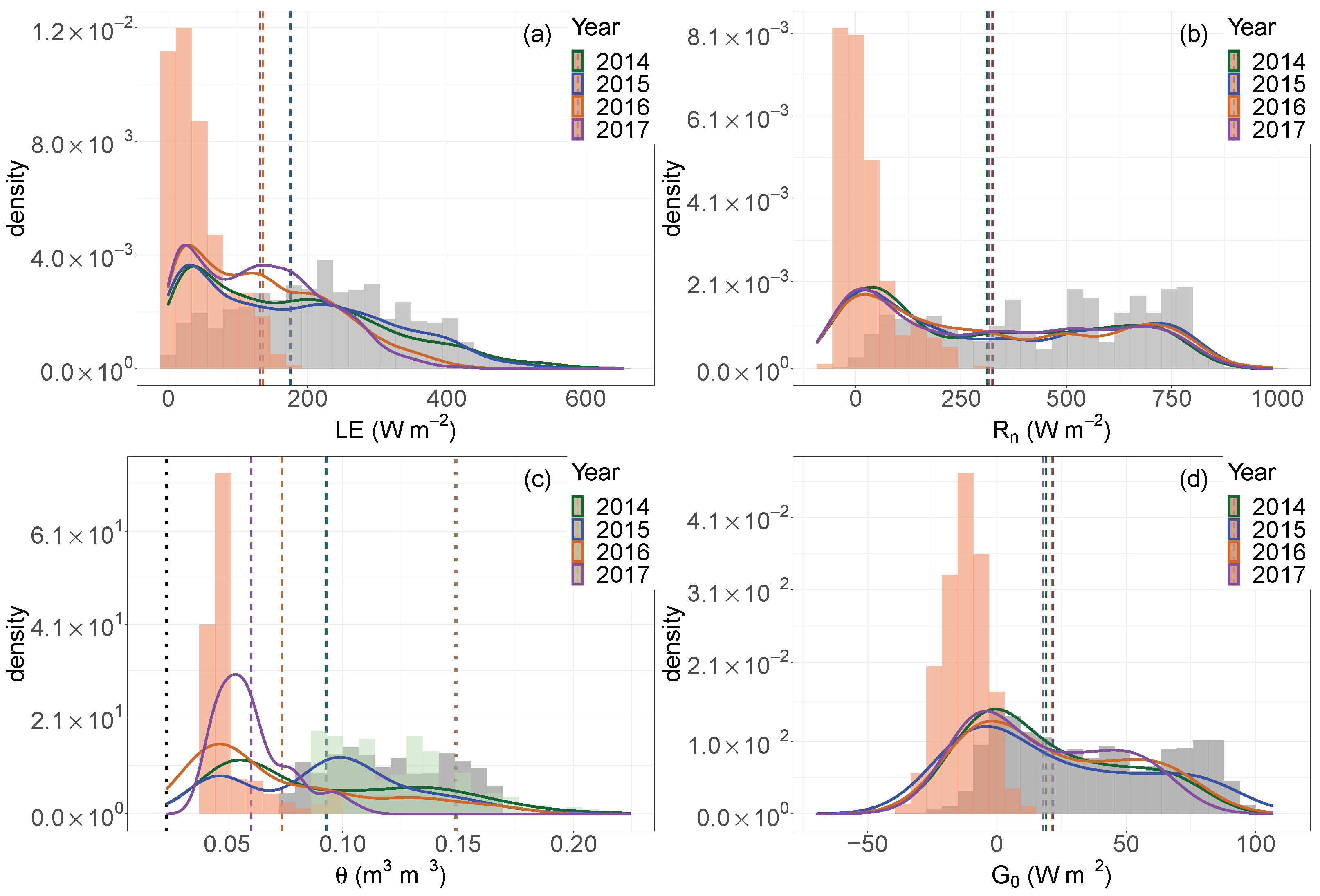
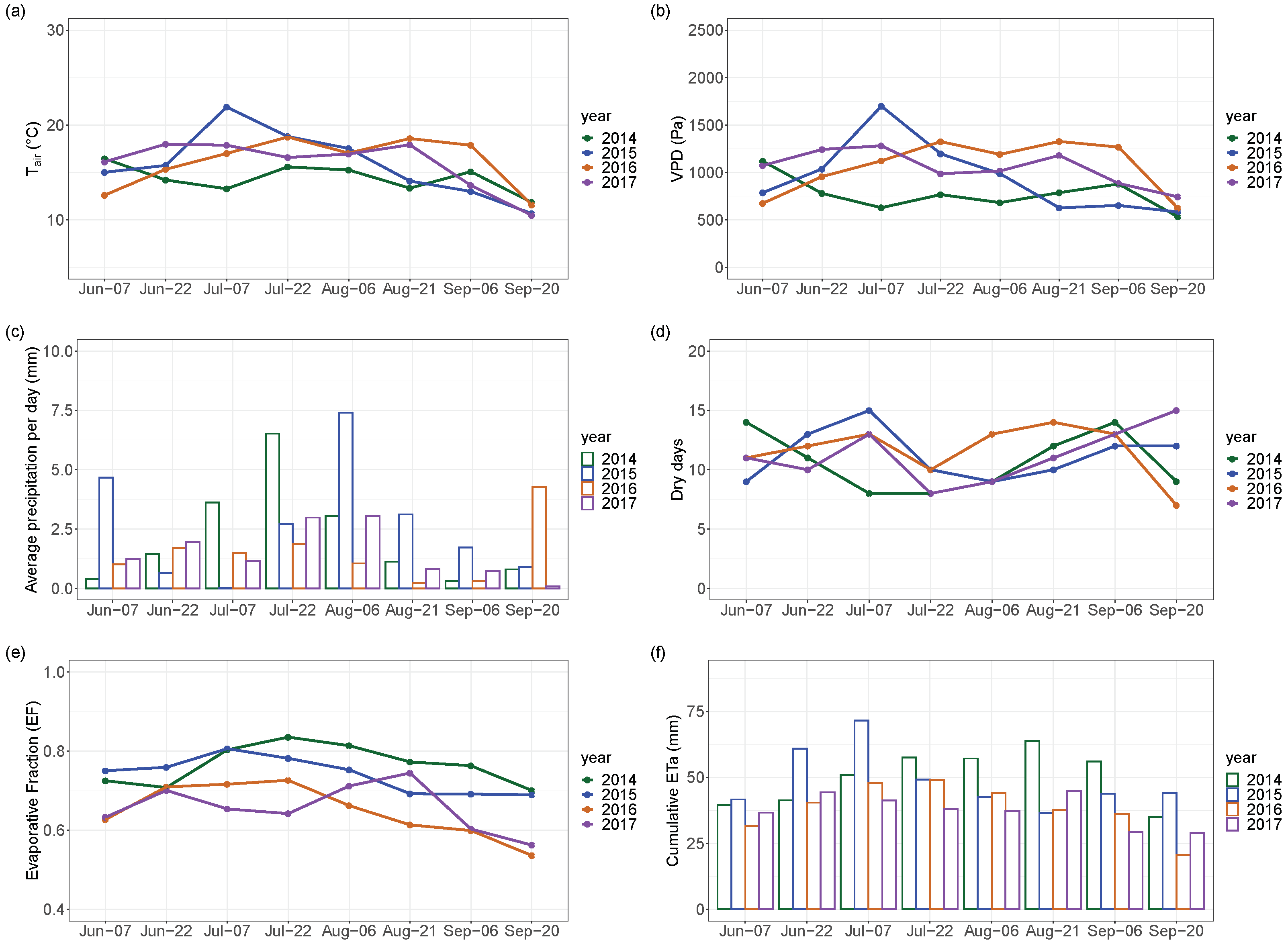
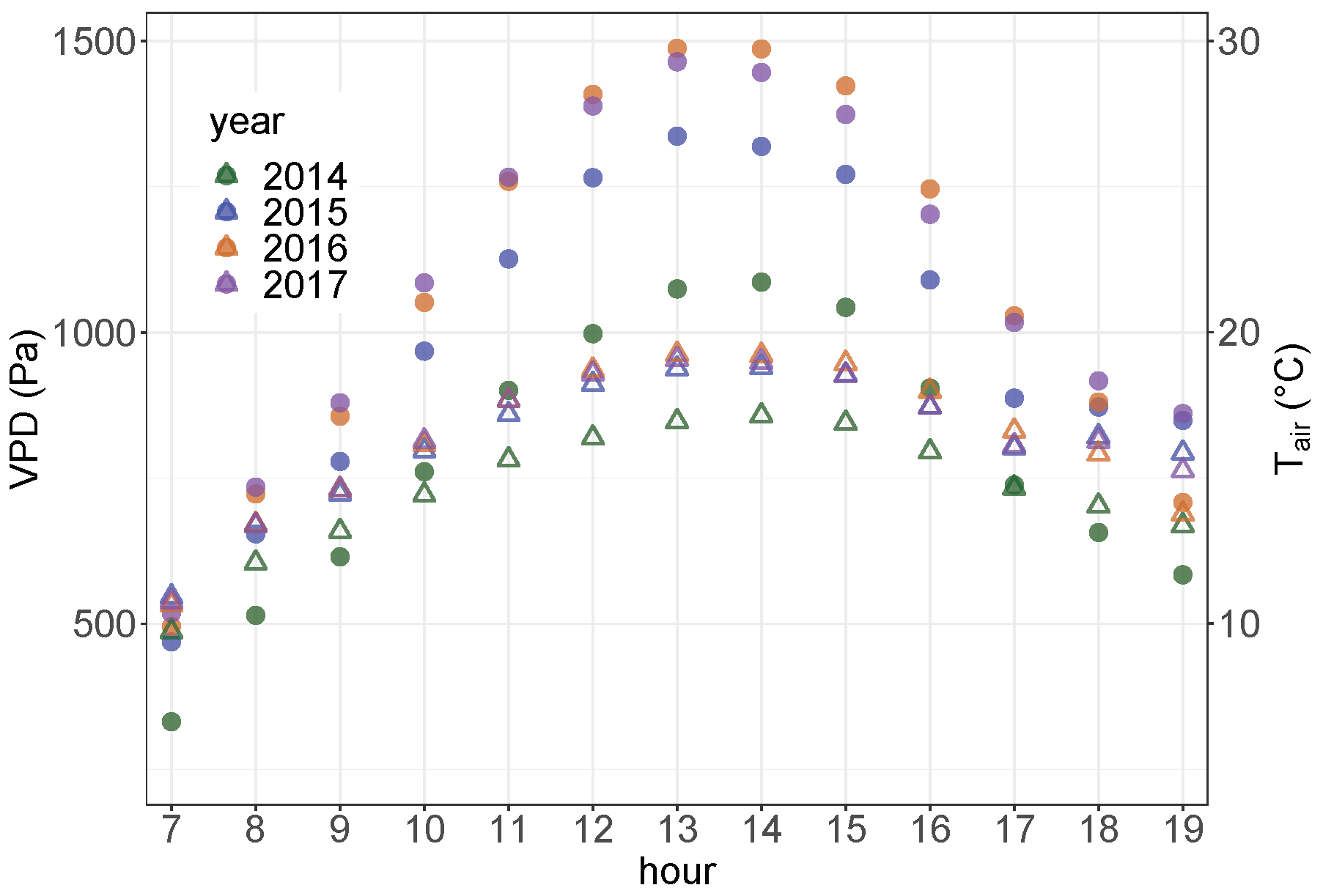
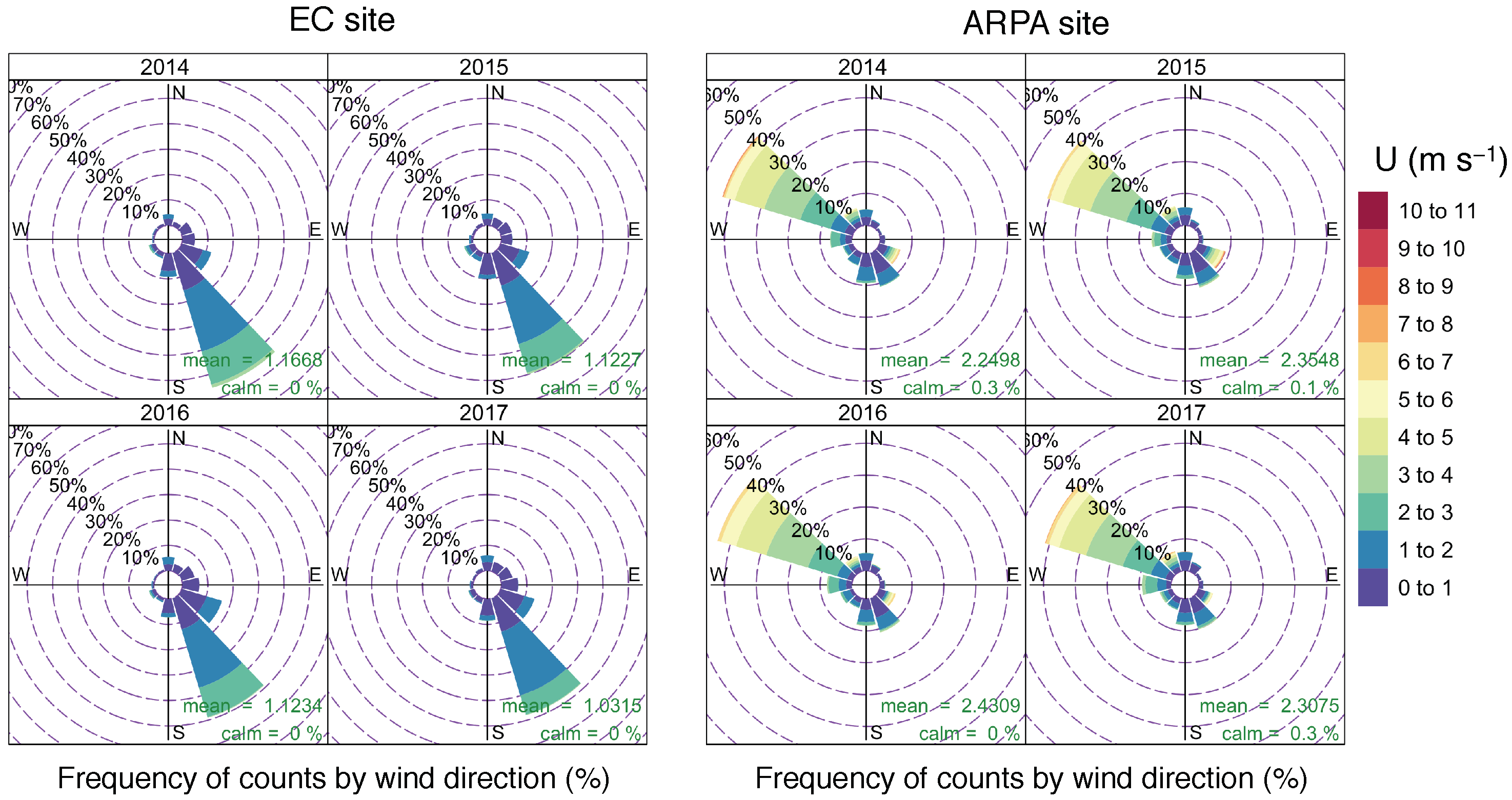
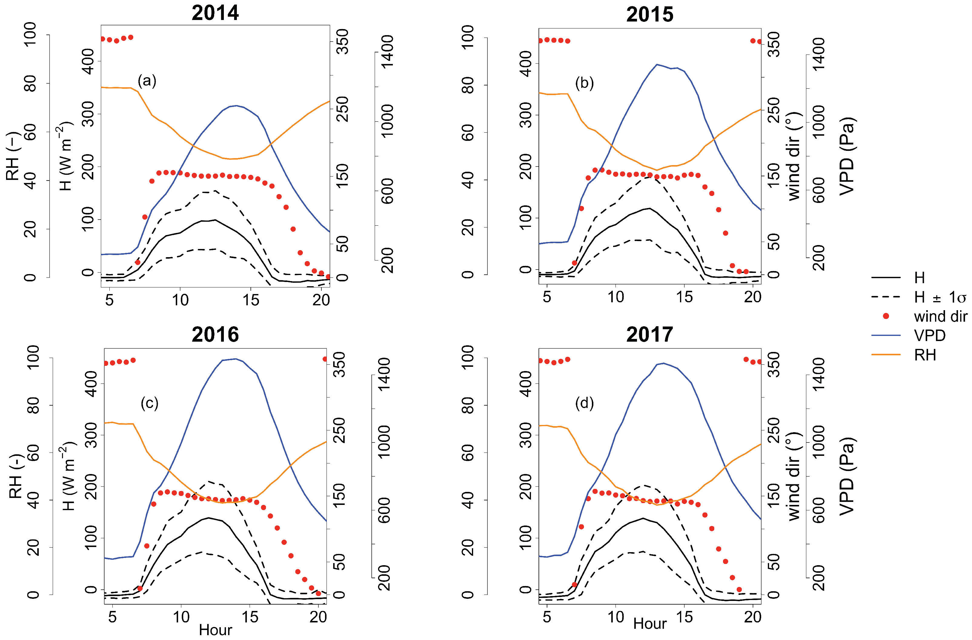
The current study deepened the knowledge of an Alpine ecosystem still poorly studied by using eddy covariance. A micrometeorological and hydrological analysis of a steep abandoned Alpine grassland colonised by shrubs and located in a narrow lateral valley was performed. The analysis involved three topics that can be important when field campaigns are performed at complex sites. 1. Influence of topography (i.e., valley orography) on actual evapotranspiration (ETa) and other environmental variables (wind speed, wind direction, air temperature and radiation forcing). 2. The intra- and inter-annual variability of ETa and other environmental variables (net radiation, air temperature, vapour pressure deficit—VPD, precipitation, wind speed, ground heat flux, soil water content). 3. The ETa drivers and their temporal variability.
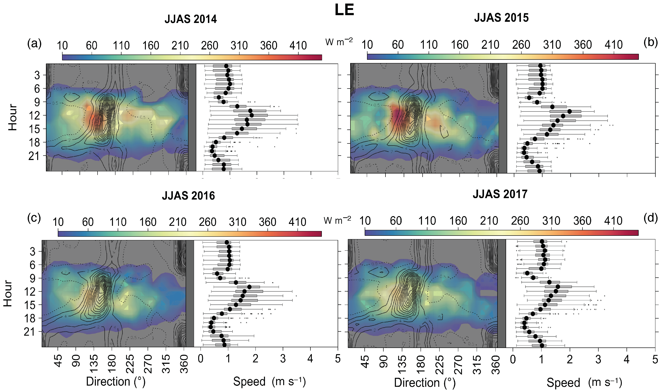
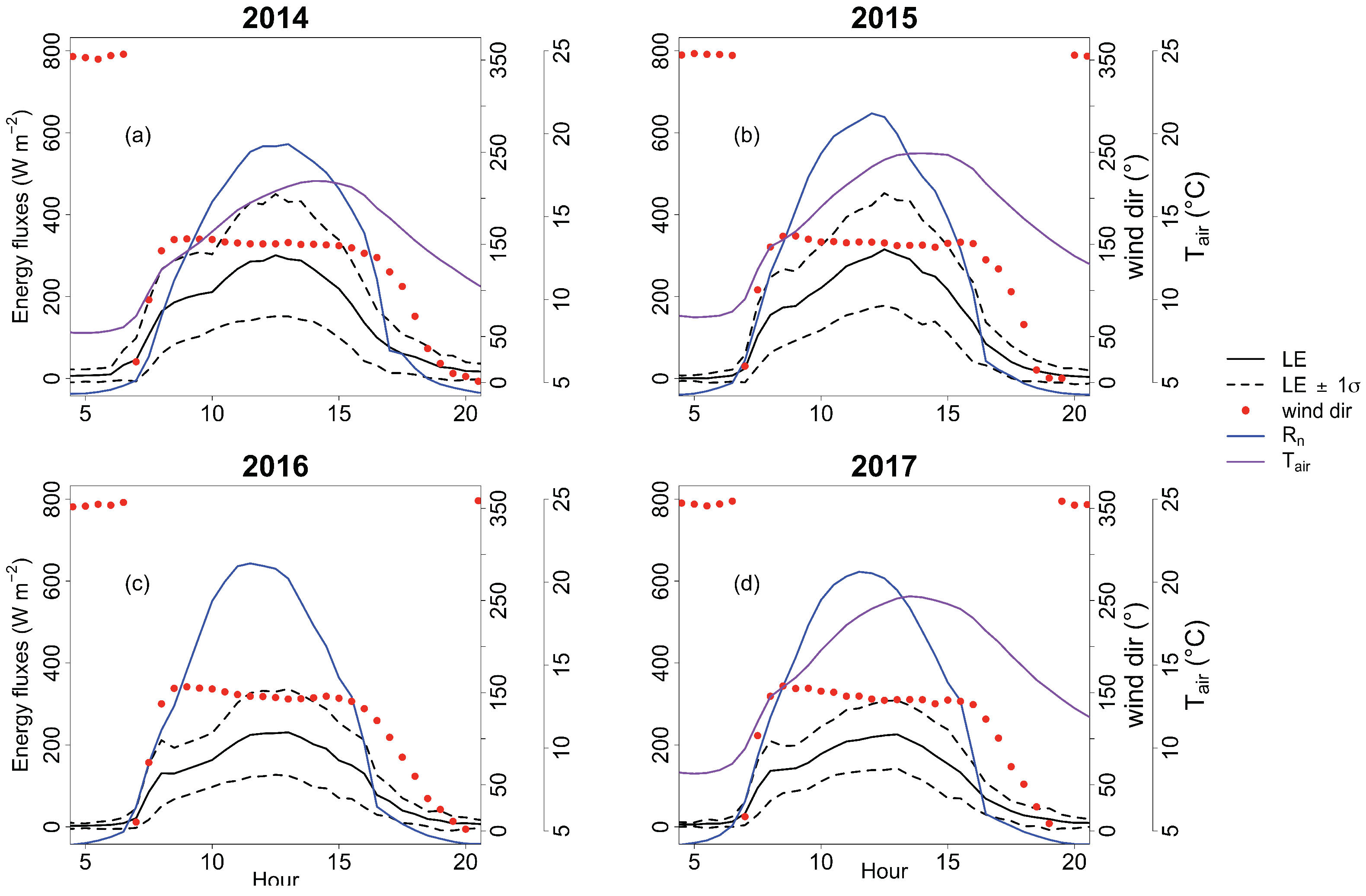
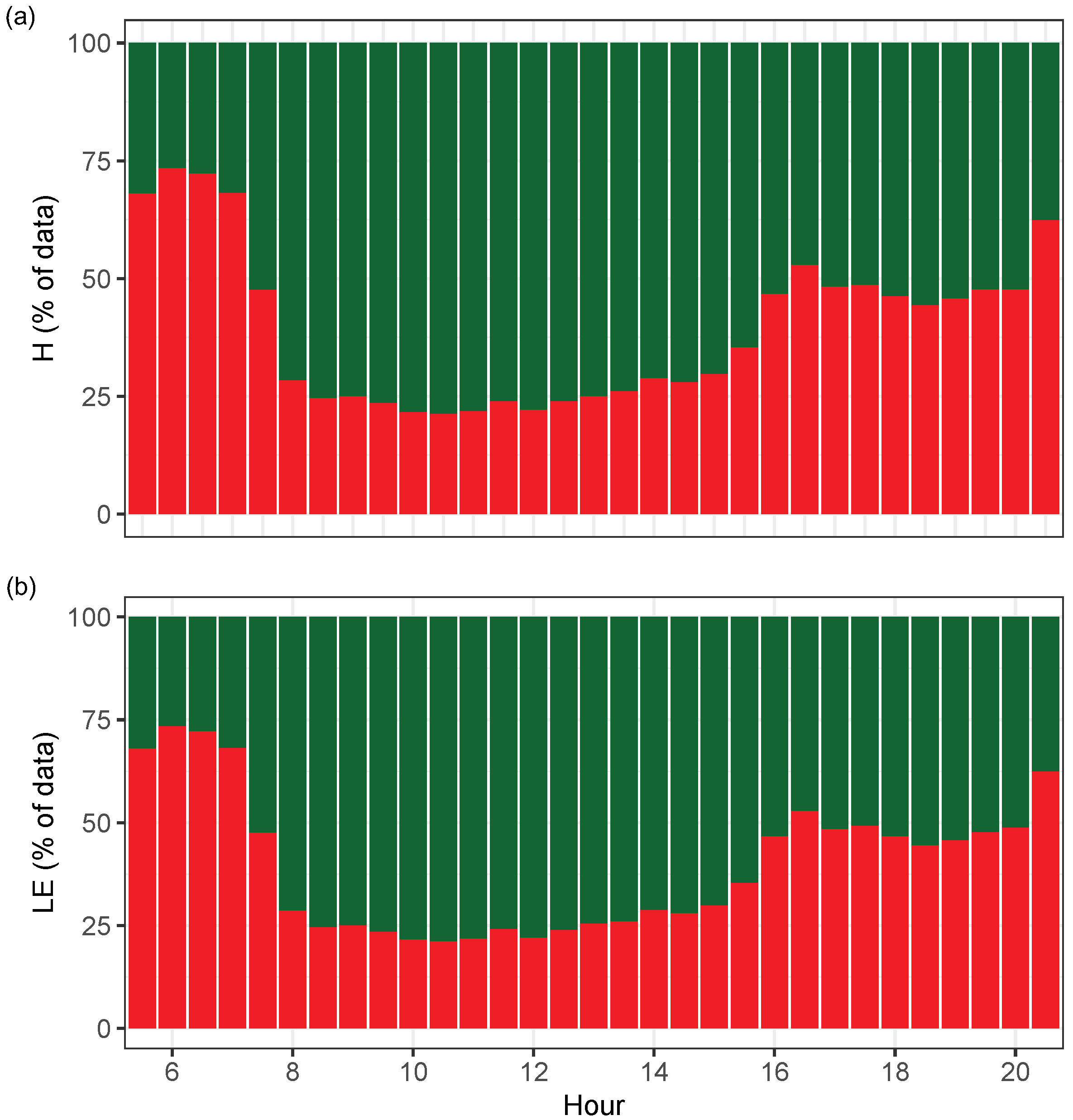
The topography of the valley produced a rarely studied inflexion visible in the mean diurnal cycle of the turbulent fluxes and ETa. Other sites with similar topographical conditions may experience the same feature, which would affect the measurements leading to a reduction of turbulent fluxes (and ETa) in the morning.
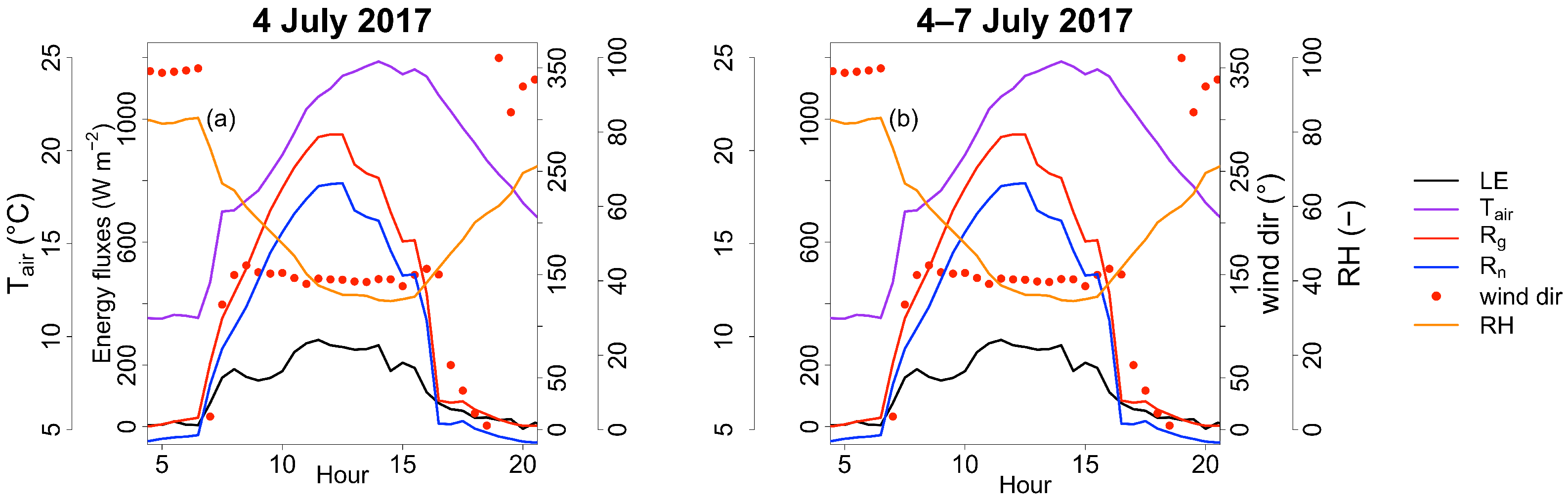
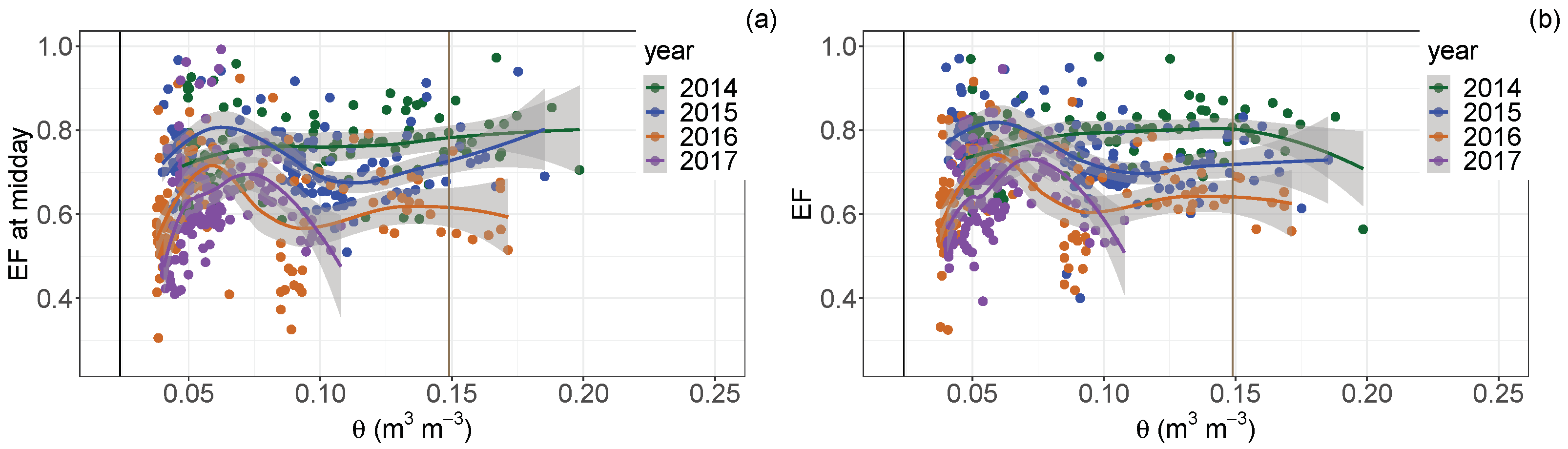
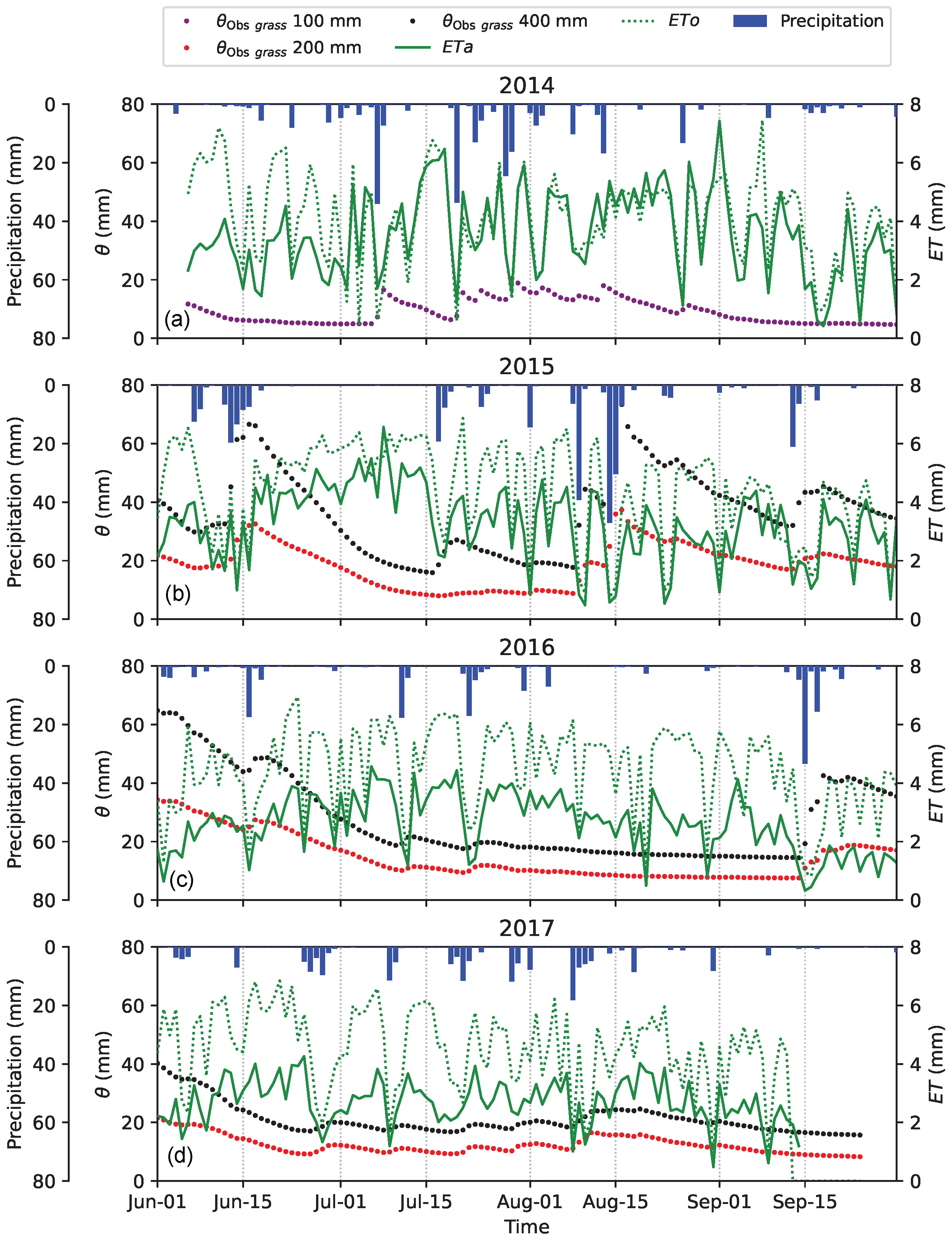
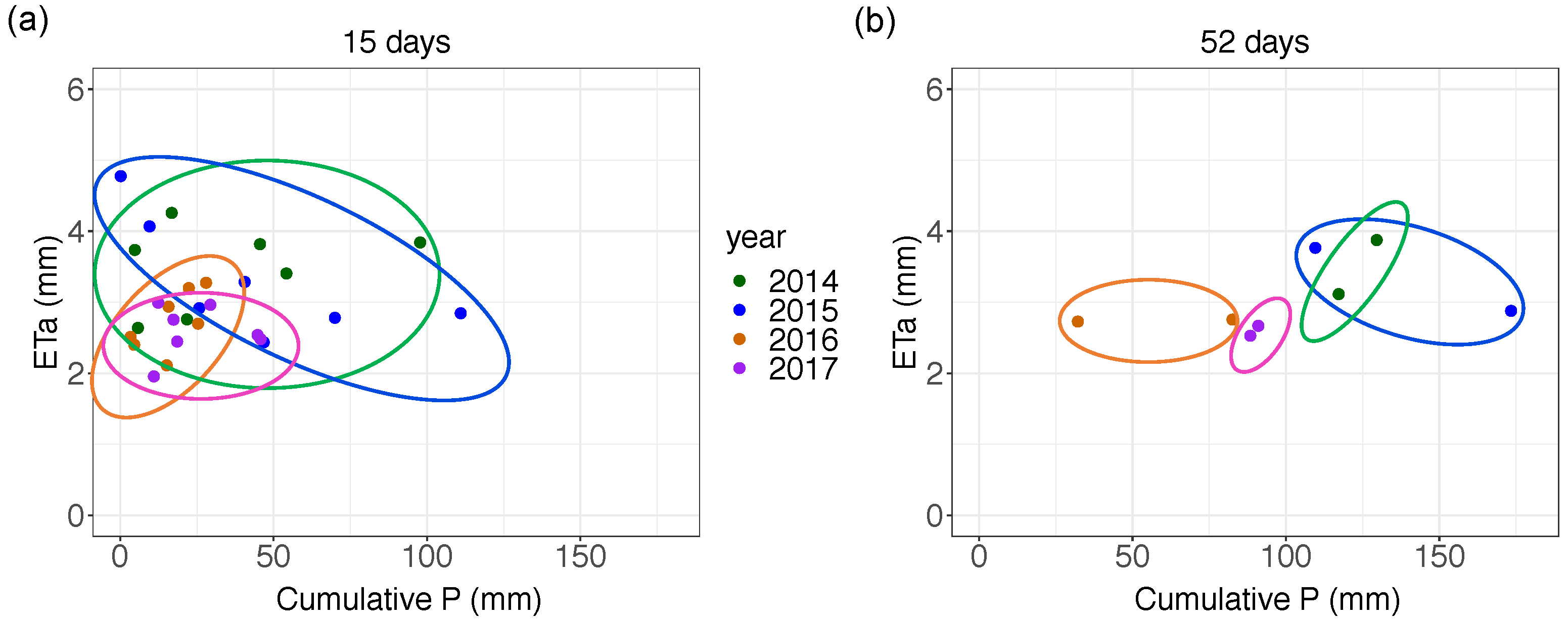
Temporal differences of ETa and the other environmental variables were found. In particular, a significant difference in ETa was detected between wet and dry growing seasons. Besides, the ETa data in wet growing seasons showed a larger variability. Considering the daytime hours, a bimodality of ETa was found in every growing season, caused by the transition from low to high radiation forcing in the morning. Energy- and water-limited regimes changed within and between growing seasons. Moreover, conditions closer to water-limited ETa were identified not only in dry growing seasons but also in an overall wet growing season characterised by a very long dry period. The distinction between the two regimes by comparing ETa with the potential evapotranspiration proved to be reliable and it could be more useful than ETa relationship with soil water content, especially if water content is measured at shallow depths. Also, the differences between wet and dry growing seasons were identified using periods of fifteen days. The analysis showed that ETa can be high in dry conditions, with high air temperature and VPD provided that vegetation with sufficient root depth exists. Enhanced ETa could also be found in wet conditions with low air temperature and VPD if a high water availability occurs.
The ETa inter-annual variability, likely also due to the existence of shrubs, emerged also from the non-negligible impact of random effects in an assumed linear mixed model of the main ETa drivers. Other studies in Alpine regions may use this methodological approach to test if their ETa data have an inter-annual variability. The most important ETa drivers for the abandoned grassland were net radiation ( R n ) and VPD, but also the wind speed (U) had to be considered. In dry and warm growing seasons, also air temperature ( T a i r ) and ground heat flux at the surface ( G 0 ) were important drivers. The weak relationship between ETa and precipitation suggested that soil water availability measurements would be a better driver than precipitation. However, the present study also highlighted that for a mixture of grassland and shrubland, deep soil water content measurements below 40 cm are necessary when the soil water content is investigated as an ETa driver.
The current study highlighted that the abandoned grasslands encroached by shrubs can have a similar behaviour compared to managed grasslands such as pastures and meadows. However, during dry and warm conditions, the presence of shrubs may significantly enhance evapotranspiration. Finally, the present study can be useful for eco-hydrological models simulations and validation as done at other sites in [102], and for further hydrological modelling analyses at the Cogne site currently in development.

Author Contributions

Conceptualization, D.G., S.F., A.K., J.v.R., L.S.; methodology, D.G., S.F., A.K., J.v.R., I.B., L.S.; software, D.G., I.B.; validation, D.G., S.F., J.v.R., A.K.; formal analysis, D.G., I.B., S.F.; investigation, D.G., S.F., D.C., M.P.; resources, S.F.; data curation, D.G., D.C., M.P., S.F.; writing: original draft preparation, D.G.; writing: review and editing, D.G., S.F., J.v.R., A.K., L.S.; visualization, D.G., I.B., S.F.; supervision, S.F. All authors have read and agreed to the published version of the manuscript.

Funding

This research was partially funded by “PRIN MIUR 2017SL7ABC_005 WATZON Project” and by “MIUR—Dipartimento di Eccellenza” DIST department funds.

Institutional Review Board Statement

Not applicable.

Informed Consent Statement

Not applicable.

Data Availability Statement

The data used in this study are available on request.

Acknowledgments

The authors would like to thank the Environmental Protection Agency of Valle d’Aosta Region (ARPA-VdA) for having provided meteorological data of their station at Cogne-Gimillan. Furthermore, the authors acknowledge Stefano Bechis for the technical support in the station installation and management. The authors thank the anonymous reviewers for their valuable comments and suggestions to improve the manuscript.

Conflicts of Interest

The authors declare no conflict of interest. The funders had no role in the design of the study, in the collection, analyses or interpretation of data; in the writing of the manuscript, or in the decision to publish the results.

Symbols and Abbreviations

SymbolVariableUnit
L E Latent heat fluxW m 2
HSensible heat fluxW m 2
R n Net radiationW m 2
R g Global radiationW m 2
GGround heat fluxW m 2
G 0 Ground heat flux at the land surfaceW m 2
S s o i l Heat storage flux above the soil heat flux platesW m 2
S c a n o p y Heat storage flux within the canopyW m 2
SOverall (soil + canopy heat storage flux)W m 2
T a i r Air temperature°C
UWind speedm s 1
RHRelative humidity(-)
VPDVapour pressure deficitPa
θ Soil water content (at 10–20 cm depth if not specified, or at 40 cm if specified)m 3 m 3
ETaActual evapotranspirationmm
EToPotential evapotranspirationmm
EFEvaporative fraction(-)
PPrecipitationmm
AbbreviationMeaning
ECEddy covariance
AICAkaike Information Criterion
AICcCorrected Akaike Information Criterion
MJJASMay-September period
JJASJune-September period (growing season)

Appendix A

Figure A1. Number of grassland stations in Europe. The blue bar indicates the altitude range in which the Cogne site is located.
Atmosphere 13 00977 g0a1
Table A1. Main experimental mountain sites on Alpine grasslands (Alps) and their characteristics.
SiteAltitudeTerrainLand UseECReference
AT-Sta1970strong slopeabandoned grasslandno[32]
AT-Stm1770strong slopemanaged meadowyes[11]
AT-Stp1850strong slopemanaged meadowno[32]
CH-Aws1978flatgrasslandyes[103]
CH-Dsc1590flatgrasslandyes[104]
CH-Frk2100strong slopegrasslandyes[105]
ES-Cst1900gentle slopegrasslandyes[106]
ES-VdA1770gentle slopemanaged meadowyes[107]
FR-Clt2000signif. slopegrasslandno[108]
IT-Mal2000gentle slopegrasslandyes[109]
IT-Mbo1550almost flatgrasslandyes[110]
IT-Mtm1500strong slopemanaged meadowyes[111]
IT-Mtp1500strong slopegrasslandyes[111]
IT-Tor2150gentle slopeabandoned grasslandyes[33]
Figure A2. Distribution of grassland areas in Aosta Valley for different altitude classes.
Atmosphere 13 00977 g0a2
Table A2. Extremes of physical plausible data for the Cogne site for wind speed anemometric components (u, v, w), sonic temperature ( T s ), CO 2 and H 2 O concentration values.
uvw T s [CO 2 ][H 2 O]
(m s 1 )(m s 1 )(m s 1 )(°C)( μ mol m 3 )(mmol m 3 )
MINMAXMINMAXMINMAXMINMAXMINMAXMINMAX
−30+30−30+30−5+5−40+5073001800
Figure A3. Mean diurnal cycles for quality control on the data set. Green: good quality data. Red: bad quality data. (a) Sensible heat flux. (b) Latent heat flux.
Atmosphere 13 00977 g0a3
Figure A4. Daytime wind roses at the eddy covariance site (left) and at the Regional Authority (ARPA-VdA) site (right). Figure done with Openair R package [112].
Atmosphere 13 00977 g0a4
Figure A5. Mean diurnal cycles of daytime sensible heat flux (H), vapour pressure deficit (VPD), relative humidity (RH) and wind direction for the four growing seasons. Half-hourly data. (a) 2014. (b) 2015. (c) 2016. (d) 2017.
Atmosphere 13 00977 g0a5
Table A3. Results of the multivariate regression of actual evapotranspiration against the considered drivers. p-Values for Student t (threshold set to 0.05) and Akaike information criterion corrected for small sample sizes (AICc) values for each growing season. Illustrated AICc values are prior to AICc stepwise minimisation.
YearDriverp-ValueAICc
2014 R n ~0306.9
VPD0.007295.1
U~0305.2
G 0 0.16289.5
T a i r 0.13289.8
2015 R n ~0164.9
VPD~0185.1
U~0153.4
G 0 0.16135.0
T a i r 0.003142.6
2016 R n ~0202.3
VPD~0134.8
U~0175.0
G 0 ~0124.1
T a i r 0.26108.9
2017 R n ~0126.5
VPD0.0366.2
U~086.1
G 0 ~085.3
T a i r 0.00172.9
Figure A6. Frequency density distributions (in every growing season) of three micrometeorological variables. (a) Wind speed (U). (b) Vapour pressure deficit. (c) Air temperature. Dashed lines represent the mean values for each variable in each growing season. Based on 2015 data as an example, light red histograms represent the density distribution between 05:00 and 7:00 and between 17:00 and 20:00. The grey histograms refer to the hours between 08:00 and 16:00.
Atmosphere 13 00977 g0a6
Figure A7. (a) Actual evapotranspiration versus average shallow soil water content (10–20 cm of depth) considering 15-days periods for each growing season. (b) Actual evapotranspiration versus average shallow soil water content (10–20 cm of depth) considering 52-days periods for each growing season. Ellipses highlight the different regions of the plane in which the data lay in different years. The cumulative actual evapotranspiration was normalised by the number of days of each considered time period.
Atmosphere 13 00977 g0a7
Figure A8. (a) Actual evapotranspiration (ETa) versus cumulative precipitation (cumulative P) considering 15, 36, 35 and 53 days periods. (b) Actual evapotranspiration (ETa) versus average shallow soil water content ( θ , 10–20 cm of depth) considering 15, 36, 35 and 52 days periods. None of the regressions is significant.
Atmosphere 13 00977 g0a8

References

  1. Lettenmaier, D.P.; Famiglietti, J.S. Hydrology: Water from on high. Nature 2006, 444, 562–563. [Google Scholar] [CrossRef] [PubMed]
  2. Coenders-Gerrits, M.; Schilperoort, B.; Jiménez-Rodríguez, C. Evaporative Processes on Vegetation: An Inside Look. In Precipitation Partitioning by Vegetation: A Global Synthesis; Van Stan, J.T.I., Gutmann, E., Friesen, J., Eds.; Springer International Publishing: Cham, Switzerland, 2020; pp. 35–48. [Google Scholar] [CrossRef]
  3. Goulden, M.L.; Bales, R.C. Mountain runoff vulnerability to increased evapotranspiration with vegetation expansion. Proc. Natl. Acad. Sci. USA 2014, 111, 14071–14075. [Google Scholar] [CrossRef] [PubMed] [Green Version]
  4. Bonan, G. Ecological Climatology: Concepts and Applications, 3rd ed.; Cambridge University Press: Cambridge, UK, 2015. [Google Scholar] [CrossRef]
  5. Sade, N.; Gebremedhin, A.; Moshelion, M. Risk-taking plants. Plant Signal. Behav. 2012, 7, 767–770. [Google Scholar] [CrossRef] [PubMed] [Green Version]
  6. Ward, H.C. Scintillometry in urban and complex environments: A review. Meas. Sci. Technol. 2017, 28, 064005. [Google Scholar] [CrossRef]
  7. Ghiat, I.; Mackey, H.R.; Al-Ansari, T. A Review of Evapotranspiration Measurement Models, Techniques and Methods for Open and Closed Agricultural Field Applications. Water 2021, 13, 2523. [Google Scholar] [CrossRef]
  8. Foken, T. Micrometeorology; Springer: Berlin/Heidelberg, Germany, 2008. [Google Scholar] [CrossRef]
  9. Geissbühler, P.; Siegwolf, R.; Eugster, W. Eddy Covariance Measurements on Mountain Slopes: The Advantage of Surface-Normal Sensor Orientation over a Vertical Set-Up. Bound.-Layer Meteorol. 2000, 96, 371–392. [Google Scholar] [CrossRef]
  10. Turnipseed, A.A.; Anderson, D.E.; Blanken, P.D.; Baugh, W.M.; Monson, R.K. Airflows and turbulent flux measurements in mountainous terrain Part 1. Canopy and local effects. Agric. For. Meteorol. 2003, 119, 1–21. [Google Scholar] [CrossRef]
  11. Hammerle, A.; Haslwanter, A.; Schmitt, M.; Bahn, M.; Tappeiner, U.; Cernusca, A.; Wohlfahrt, G. Eddy covariance measurements of carbon dioxide, latent and sensible energy fluxes above a meadow on a mountain slope. Bound.-Layer Meteorol. 2007, 122, 397–416. [Google Scholar] [CrossRef] [Green Version]
  12. Stiperski, I.; Rotach, M.W. On the Measurement of Turbulence Over Complex Mountainous Terrain. Bound.-Layer Meteorol. 2016, 159, 97–121. [Google Scholar] [CrossRef] [Green Version]
  13. Golzio, A.; Bollati, I.M.; Ferrarese, S. An Assessment of Coordinate Rotation Methods in Sonic Anemometer Measurements of Turbulent Fluxes over Complex Mountainous Terrain. Atmosphere 2019, 10, 324. [Google Scholar] [CrossRef] [Green Version]
  14. Hiller, R.; Zeeman, M.J.; Eugster, W. Eddy-Covariance Flux Measurements in the Complex Terrain of an Alpine Valley in Switzerland. Bound.-Layer Meteorol. 2008, 127, 449–467. [Google Scholar] [CrossRef] [Green Version]
  15. Mauder, M.; Cuntz, M.; Drüe, C.; Graf, A.; Rebmann, C.; Schmid, H.P.; Schmidt, M.; Steinbrecher, R. A strategy for quality and uncertainty assessment of long-term eddy-covariance measurements. Agric. For. Meteorol. 2013, 169, 122–135. [Google Scholar] [CrossRef]
  16. Wohlfahrt, G.; Hammerle, A.; Niedrist, G.; Scholz, K.; Tomelleri, E.; Zhao, P. On the energy balance closure and net radiation in complex terrain. Agric. For. Meteorol. 2016, 226–227, 37–49. [Google Scholar] [CrossRef] [Green Version]
  17. Moncrieff, J.; Clement, R.; Finnigan, J.; Meyers, T. Averaging, Detrending, and Filtering of Eddy Covariance Time Series. In Handbook of Micrometeorology: A Guide for Surface Flux Measurement and Analysis; Lee, X., Massman, W., Law, B., Eds.; Atmospheric and Oceanographic Sciences Library; Springer: Dordrecht, The Netherlands, 2005; pp. 7–31. [Google Scholar] [CrossRef]
  18. Lee, X.; Finnigan, J.; Paw U, K.T. Coordinate Systems and Flux Bias Error. In Handbook of Micrometeorology: A Guide for Surface Flux Measurement and Analysis; Lee, X., Massman, W., Law, B., Eds.; Atmospheric and Oceanographic Sciences Library; Springer: Dordrecht, The Netherlands, 2005; pp. 33–66. [Google Scholar] [CrossRef]
  19. Foken, T.; Göockede, M.; Mauder, M.; Mahrt, L.; Amiro, B.; Munger, W. Post-Field Data Quality Control. In Handbook of Micrometeorology: A Guide for Surface Flux Measurement and Analysis; Lee, X., Massman, W., Law, B., Eds.; Atmospheric and Oceanographic Sciences Library; Springer: Dordrecht, The Netherlands, 2005; pp. 181–208. [Google Scholar] [CrossRef]
  20. Vickers, D.; Mahrt, L. Quality Control and Flux Sampling Problems for Tower and Aircraft Data. J. Atmos. Ocean. Technol. 1997, 14, 512–526. [Google Scholar] [CrossRef]
  21. Foken, T.; Wichura, B. Tools for quality assessment of surface-based flux measurements. Agric. For. Meteorol. 1996, 78, 83–105. [Google Scholar] [CrossRef]
  22. Mann, J.; Lenschow, D.H. Errors in airborne flux measurements. J. Geophys. Res. Atmos. 1994, 99, 14519–14526. [Google Scholar] [CrossRef]
  23. Finkelstein, P.L.; Sims, P.F. Sampling error in eddy correlation flux measurements. J. Geophys. Res. Atmos. 2001, 106, 3503–3509. [Google Scholar] [CrossRef]
  24. Göckede, M.; Rebmann, C.; Foken, T. A combination of quality assessment tools for eddy covariance measurements with footprint modelling for the characterisation of complex sites. Agric. For. Meteorol. 2004, 127, 175–188. [Google Scholar] [CrossRef]
  25. Mauder, M.; Foken, T. Documentation and Instruction Manual of the Eddy-Covariance Software Package TK3. Arbeitsergebnisse Univ. Bayreuth. Abt. Mikrometeorol. 2015, 62, 62. [Google Scholar]
  26. Wilson, S. Grasses and grassland ecology. Ann. Bot. 2009, 104, ix. [Google Scholar] [CrossRef] [Green Version]
  27. Orlandi, S.; Probo, M.; Sitzia, T.; Trentanovi, G.; Garbarino, M.; Lombardi, G.; Lonati, M. Environmental and land use determinants of grassland patch diversity in the western and eastern Alps under agro-pastoral abandonment. Biodivers. Conserv. 2016, 25, 275–293. [Google Scholar] [CrossRef]
  28. Komac, B.; Alados, C.L.; Camarero, J.J. Influence of Topography on the Colonization of Subalpine Grasslands by the Thorny Cushion Dwarf Echinospartum horridum. Arct. Antarct. Alp. Res. 2011, 43, 601–611. [Google Scholar] [CrossRef] [Green Version]
  29. van den Bergh, T.; Körner, C.; Hiltbrunner, E. Alnus shrub expansion increases evapotranspiration in the Swiss Alps. Reg. Environ. Chang. 2018, 18, 1375–1385. [Google Scholar] [CrossRef]
  30. Fluxnet Sites Network. Available online: https://fluxnet.org/sites/site-list-and-pages/ (accessed on 25 April 2022).
  31. European Fluxes Database Cluster. Available online: http://www.europe-fluxdata.eu/ (accessed on 25 April 2022).
  32. Tenhunen, J.; Geyer, R.; Adiku, S.; Reichstein, M.; Tappeiner, U.; Bahn, M.; Cernusca, A.; Dinh, N.Q.; Kolcun, O.; Lohila, A.; et al. Influences of changing land use and CO2 concentration on ecosystem and landscape level carbon and water balances in mountainous terrain of the Stubai Valley, Austria. Glob. Planet. Chang. 2009, 67, 29–43. [Google Scholar] [CrossRef]
  33. Galvagno, M.; Wohlfahrt, G.; Cremonese, E.; Filippa, G.; Migliavacca, M.; Mora di Cella, U.; van Gorsel, E. Contribution of advection to nighttime ecosystem respiration at a mountain grassland in complex terrain. Agric. For. Meteorol. 2017, 237–238, 270–281. [Google Scholar] [CrossRef]
  34. Xhao, X.; Liu, Y. Relative Contribution of the Topographic Influence on the Triangle Approach for Evapotranspiration Estimation over Mountainous Areas. Adv. Meteorol. 2014, 2014, 584040. [Google Scholar] [CrossRef]
  35. Liu, M.; Bárdossy, A.; Li, J.; Jiang, Y. Physically-based modeling of topographic effects on spatial evapotranspiration and soil moisture patterns through radiation and wind. Hydrol. Earth Syst. Sci. 2012, 16, 357–373. [Google Scholar] [CrossRef] [Green Version]
  36. Gisolo, D.; Previati, M.; Canone, D.; Boetti, M.; Dematteis, N.; Balocco, J.; Ferrari, S.; Gentile, A.; Nsassila, M.; Heery, B.; et al. A calibrationless radiation driven model for estimating actual evapotranspiration of mountain grasslands. J. Hydrol. 2022, 610, 127948. [Google Scholar] [CrossRef]
  37. Rotach, M.W.; Calanca, P.; Graziani, G.; Gurtz, J.; Steyn, D.G.; Vogt, R.; Andretta, M.; Christen, A.; Cieslik, S.; Connolly, R.; et al. Turbulence Structure and Exchange Processes in an Alpine Valley: The Riviera Project. Bull. Am. Meteorol. Soc. 2004, 85, 1367–1386. [Google Scholar] [CrossRef] [Green Version]
  38. Rotach, M.W.; Andretta, M.; Calanca, P.; Weigel, A.P.; Weiss, A. Boundary layer characteristics and turbulent exchange mechanisms in highly complex terrain. Acta Geophys. 2008, 56, 194–219. [Google Scholar] [CrossRef]
  39. Sfyri, E.; Rotach, M.W.; Stiperski, I.; Bosveld, F.C.; Lehner, M.; Obleitner, F. Scalar-Flux Similarity in the Layer Near the Surface Over Mountainous Terrain. Bound.-Layer Meteorol. 2018, 169, 11–46. [Google Scholar] [CrossRef] [PubMed] [Green Version]
  40. Liang, J.; Guo, Q.; Zhang, Z.; Zhang, M.; Tian, P.; Zhang, L. Influence of Complex Terrain on Near-Surface Turbulence Structures over Loess Plateau. Atmosphere 2020, 11, 930. [Google Scholar] [CrossRef]
  41. Rotach, M.W.; Stiperski, I.; Fuhrer, O.; Goger, B.; Gohm, A.; Obleitner, F.; Rau, G.; Sfyri, E.; Vergeiner, J. Investigating Exchange Processes over Complex Topography: The Innsbruck Box (i-Box). Bull. Am. Meteorol. Soc. 2017, 98, 787–805. [Google Scholar] [CrossRef]
  42. Wieser, G.; Hammerle, A.; Wohlfahrt, G. The Water Balance of Grassland Ecosystems in the Austrian Alps. Arct. Antarct. Alp. Res. 2008, 40, 439–445. [Google Scholar] [CrossRef]
  43. Ryu, Y.; Baldocchi, D.D.; Ma, S.; Hehn, T. Interannual variability of evapotranspiration and energy exchange over an annual grassland in California. J. Geophys. Res. Atmos. 2008, 113, D09104. [Google Scholar] [CrossRef] [Green Version]
  44. Wever, L.A.; Flanagan, L.B.; Carlson, P.J. Seasonal and interannual variation in evapotranspiration, energy balance and surface conductance in a northern temperate grassland. Agric. For. Meteorol. 2002, 112, 31–49. [Google Scholar] [CrossRef]
  45. Gu, S.; Tang, Y.; Cui, X.; Du, M.; Zhao, L.; Li, Y.; Xu, S.; Zhou, H.; Kato, T.; Qi, P.; et al. Characterizing evapotranspiration over a meadow ecosystem on the Qinghai-Tibetan Plateau. J. Geophys. Res. Atmos. 2008, 113, D08118. [Google Scholar] [CrossRef]
  46. Wu, H.; Li, X.Y.; Li, J.; Zhang, C.; He, B.; Zhang, S.; Sun, W. Age-related water uptake patterns of alpine plantation shrubs in reforestation region of Qinghai–Tibetan Plateau based on stable isotopes. Ecohydrology 2019, 12, e2049. [Google Scholar] [CrossRef] [Green Version]
  47. Huizhi, L.; Jianwu, F. Seasonal and Interannual Variations of Evapotranspiration and Energy Exchange over Different Land Surfaces in a Semiarid Area of China. J. Appl. Meteorol. Climatol. 2012, 51, 1875–1888. [Google Scholar] [CrossRef]
  48. Coners, H.; Babel, W.; Willinghöfer, S.; Biermann, T.; Köhler, L.; Seeber, E.; Foken, T.; Ma, Y.; Yang, Y.; Miehe, G.; et al. Evapotranspiration and water balance of high-elevation grassland on the Tibetan Plateau. J. Hydrol. 2016, 533, 557–566. [Google Scholar] [CrossRef]
  49. Zha, T.; Barr, A.G.; van der Kamp, G.; Black, T.A.; McCaughey, J.H.; Flanagan, L.B. Interannual variation of evapotranspiration from forest and grassland ecosystems in western canada in relation to drought. Agric. For. Meteorol. 2010, 150, 1476–1484. [Google Scholar] [CrossRef]
  50. Mackay, D.S.; Ewers, B.E.; Cook, B.D.; Davis, K.J. Environmental drivers of evapotranspiration in a shrub wetland and an upland forest in northern Wisconsin. Water Resour. Res. 2007, 43, W03442. [Google Scholar] [CrossRef] [Green Version]
  51. Detsch, F.; Otte, I.; Appelhans, T.; Nauss, T. A glimpse at short-term controls of evapotranspiration along the southern slopes of Kilimanjaro. Environ. Monit. Assess. 2017, 189, 465. [Google Scholar] [CrossRef] [PubMed]
  52. Kang, T.; Li, Z.; Gao, Y. Spatiotemporal Variations of Reference Evapotranspiration and Its Determining Climatic Factors in the Taihang Mountains, China. Water 2021, 13, 3145. [Google Scholar] [CrossRef]
  53. Moncrieff, J.B.; Massheder, J.M.; de Bruin, H.; Elbers, J.; Friborg, T.; Heusinkveld, B.; Kabat, P.; Scott, S.; Soegaard, H.; Verhoef, A. A system to measure surface fluxes of momentum, sensible heat, water vapour and carbon dioxide. J. Hydrol. 1997, 188–189, 589–611. [Google Scholar] [CrossRef]
  54. Webb, E.K.; Pearman, G.I.; Leuning, R. Correction of flux measurements for density effects due to heat and water vapour transfer. Q. J. R. Meteorol. Soc. 1980, 106, 85–100. [Google Scholar] [CrossRef]
  55. Schotanus, P.; Nieuwstadt, F.; De Bruin, H. Temperature measurement with a sonic anemometer and its application to heat and moisture fluxes. Bound.-Layer Meteorol. 1983, 26, 81–93. [Google Scholar] [CrossRef]
  56. Fan, S.M.; Wofsy, S.C.; Bakwin, P.S.; Jacob, D.J.; Fitzjarrald, D.R. Atmosphere-biosphere exchange of CO2 and O3 in the central Amazon Forest. J. Geophys. Res. Atmos. 1990, 95, 16851–16864. [Google Scholar] [CrossRef]
  57. Papale, D.; Reichstein, M.; Aubinet, M.; Canfora, E.; Bernhofer, C.; Kutsch, W.; Longdoz, B.; Rambal, S.; Valentini, R.; Vesala, T.; et al. Towards a standardized processing of Net Ecosystem Exchange measured with eddy covariance technique: Algorithms and uncertainty estimation. Biogeosciences 2006, 3, 571–583. [Google Scholar] [CrossRef] [Green Version]
  58. Van Genuchten, M.T. A Closed-form Equation for Predicting the Hydraulic Conductivity of Unsaturated Soils. Soil Sci. Soc. Am. J. 1980, 44, 892–898. [Google Scholar] [CrossRef] [Green Version]
  59. Schaap, M.G.; Leij, F.J.; van Genuchten, M.T. ROSETTA: A computer program for estimating soil hydraulic parameters with hierarchical pedotransfer functions. J. Hydrol. 2001, 251, 163–176. [Google Scholar] [CrossRef]
  60. Raffelli, G.; Previati, M.; Canone, D.; Gisolo, D.; Bevilacqua, I.; Capello, G.; Biddoccu, M.; Cavallo, E.; Deiana, R.; Cassiani, G.; et al. Local- and Plot-Scale Measurements of Soil Moisture: Time and Spatially Resolved Field Techniques in Plain, Hill and Mountain Sites. Water 2017, 9, 706. [Google Scholar] [CrossRef]
  61. German, E.R. Regional Evaluation of Evapotranspiration in the Everglades; Report 2000-4217; US Department of the Interior, US Geological Survey: Reston, VA, USA, 2000. [CrossRef]
  62. Ochsner, T. Rain or Shine; Oklahoma State University Libraries: Stillwater, OK, USA, 2019. [Google Scholar] [CrossRef]
  63. Lowe, P.R. An Approximating Polynomial for the Computation of Saturation Vapor Pressure. J. Appl. Meteorol. Climatol. 1977, 16, 100–103. [Google Scholar] [CrossRef] [Green Version]
  64. Legendre, P. Package “lmodel2”. 2018. Available online: https://cran.r-project.org/web/packages/lmodel2/ (accessed on 25 April 2022).
  65. Wilson, K.; Goldstein, A.; Falge, E.; Aubinet, M.; Baldocchi, D.; Berbigier, P.; Bernhofer, C.; Ceulemans, R.; Dolman, H.; Field, C.; et al. Energy balance closure at FLUXNET sites. Agric. For. Meteorol. 2002, 113, 223–243. [Google Scholar] [CrossRef] [Green Version]
  66. Mauder, M.; Genzel, S.; Fu, J.; Kiese, R.; Soltani, M.; Steinbrecher, R.; Zeeman, M.; Banerjee, T.; De Roo, F.; Kunstmann, H. Evaluation of energy balance closure adjustment methods by independent evapotranspiration estimates from lysimeters and hydrological simulations. Hydrol. Process. 2018, 32, 39–50. [Google Scholar] [CrossRef]
  67. Pan, X.; Liu, Y.; Fan, X.; Gan, G. Two energy balance closure approaches: Applications and comparisons over an oasis-desert ecotone. J. Arid Land 2017, 9, 51–64. [Google Scholar] [CrossRef] [Green Version]
  68. Wutzler, T.; Lucas-Moffat, A.; Migliavacca, M.; Knauer, J.; Sickel, K.; Šigut, L.; Menzer, O.; Reichstein, M. Basic and extensible post-processing of eddy covariance flux data with REddyProc. Biogeosciences 2018, 15, 5015–5030. [Google Scholar] [CrossRef] [Green Version]
  69. Reichstein, M.; Falge, E.; Baldocchi, D.; Papale, D.; Aubinet, M.; Berbigier, P.; Bernhofer, C.; Buchmann, N.; Gilmanov, T.; Granier, A.; et al. On the separation of net ecosystem exchange into assimilation and ecosystem respiration: Review and improved algorithm. Glob. Chang. Biol. 2005, 11, 1424–1439. [Google Scholar] [CrossRef]
  70. Kljun, N.; Calanca, P.; Rotach, M.W.; Schmid, H.P. A simple two-dimensional parameterisation for Flux Footprint Prediction (FFP). Geosci. Model Dev. 2015, 8, 3695–3713. [Google Scholar] [CrossRef] [Green Version]
  71. Copernicus Data Repository, ERA5 Hourly Data on Pressure Levels from 1979 to Present. Available online: https://cds.climate.copernicus.eu/cdsapp#!/dataset/reanalysis-era5-pressure-levels?tab=overviewl (accessed on 25 April 2022).
  72. R Core Team. Package “Stats”. 2021. Available online: https://stat.ethz.ch/R-manual/R-devel/library/stats/html/00Index.html (accessed on 25 April 2022).
  73. Dormann, C.F.; Elith, J.; Bacher, S.; Buchmann, C.; Carl, G.; Carré, G.; Marquéz, J.R.G.; Gruber, B.; Lafourcade, B.; Leitão, P.J.; et al. Collinearity: A review of methods to deal with it and a simulation study evaluating their performance. Ecography 2013, 36, 27–46. [Google Scholar] [CrossRef]
  74. Bates, D.; Maechler, M.; Bolker, B.; Walker, S.; Haubo Bojesen Christensen, R.; Singmann, H.; Dai, B.; Scheipl, F.; Grothendieck, G.; Green, P. Package “lme4”. 2021. Available online: https://cran.r-project.org/web/packages/lme4/index.html (accessed on 25 April 2022).
  75. Nakagawa, S.; Johnson, P.C.; Schielzeth, H. The coefficient of determination R2 and intra-class correlation coefficient from generalized linear mixed-effects models revisited and expanded. J. R. Soc. Interface 2017, 14, 20170213. [Google Scholar] [CrossRef] [PubMed] [Green Version]
  76. Barton, K. Package “MuMIn”. 2021. Available online: https://cran.r-project.org/web/packages/MuMIn/index.html (accessed on 25 April 2022).
  77. James, G.; Witten, D.; Hastie, T.; Tibshirani, R. An Introduction to Statistical Learning: With Applications in R; Springer Texts in Statistics; Springer: New York, NY, USA, 2013. [Google Scholar] [CrossRef]
  78. Ripley, B.; Venables, B.; Bates, D.M.; Hornik, K.; Gebhardt, A.; Firth, D. MASS: Support Functions and Datasets for Venables and Ripley’s MASS. 2021. Available online: https://cran.r-project.org/package=MASS (accessed on 25 April 2022).
  79. Burnham, P.K.; Anderson, R.D. Model Selection and Multimodel Inference: A Practical Information-Theoretic Approach; Springer Science & Business Media: New York, NY, USA, 2003. [Google Scholar]
  80. Mortarini, L.; Ferrero, E.; Falabino, S.; Trini Castelli, S.; Richiardone, R.; Anfossi, D. Low-frequency processes and turbulence structure in a perturbed boundary layer. Q. J. R. Meteorol. Soc. 2013, 139, 1059–1072. [Google Scholar] [CrossRef] [Green Version]
  81. Appelhans, T. Package “Metvurst”. 2019. Available online: https://github.com/tim-salabim/metvurst (accessed on 25 April 2022).
  82. Baiamonte, G.; Ferraris, S. Modelling the frequency distribution of interarrival times from daily precipitation time-series in North-West Italy. Hydrol. Res. 2018, 50, 339–357. [Google Scholar] [CrossRef] [Green Version]
  83. Cleveland, W.S.; Grosse, E.; Shyu, W.M. Local Regression Models. In Statistical Models in S; Routledge: London, UK, 1992. [Google Scholar]
  84. Allen, R.; Pereira, L.; Raes, D.; Smith, M. FAO Irrigation and drainage paper No. 56. Rome Food Agric. Organ. U. N. 1998, 56, 26–40. [Google Scholar]
  85. Zardi, D.; Whiteman, C.D. Diurnal Mountain Wind Systems. In Mountain Weather Research and Forecasting; Chow, F.K., De Wekker, S.F., Snyder, B.J., Eds.; Springer: Dordrecht, The Netherlands, 2013; pp. 35–119. [Google Scholar] [CrossRef]
  86. Yan, C.; Wang, B.; Xiang, J.; Du, J.; Zhang, S.; Qiu, G.Y. Seasonal and interannual variability of surface energy fluxes and evapotranspiration over a subalpine horizontal flow wetland in China. Agric. For. Meteorol. 2020, 288–289, 107996. [Google Scholar] [CrossRef]
  87. Aires, L.M.; Pio, C.A.; Pereira, J.S. The effect of drought on energy and water vapour exchange above a mediterranean C3/C4 grassland in Southern Portugal. Agric. For. Meteorol. 2008, 148, 565–579. [Google Scholar] [CrossRef] [Green Version]
  88. Gao, Y.; Zhao, C.; Ashiq, M.W.; Wang, Q.; Rong, Z.; Liu, J.; Mao, Y.; Guo, Z.; Wang, W. Actual evapotranspiration of subalpine meadows in the Qilian Mountains, Northwest China. J. Arid Land 2019, 11, 371–384. [Google Scholar] [CrossRef] [Green Version]
  89. Zhu, G.; Su, Y.; Li, X.; Zhang, K.; Li, C.; Ning, N. Modelling evapotranspiration in an alpine grassland ecosystem on Qinghai-Tibetan plateau. Hydrol. Process. 2014, 28, 610–619. [Google Scholar] [CrossRef]
  90. Mastrotheodoros, T.; Pappas, C.; Molnar, P.; Burlando, P.; Manoli, G.; Parajka, J.; Rigon, R.; Szeles, B.; Bottazzi, M.; Hadjidoukas, P.; et al. More green and less blue water in the Alps during warmer summers. Nat. Clim. Chang. 2020, 10, 155–161. [Google Scholar] [CrossRef]
  91. Massmann, A.; Gentine, P.; Lin, C. When Does Vapor Pressure Deficit Drive or Reduce Evapotranspiration? J. Adv. Model. Earth Syst. 2019, 11, 3305–3320. [Google Scholar] [CrossRef] [Green Version]
  92. Chen, J.; Shao, C.; Jiang, S.; Qu, L.; Zhao, F.; Dong, G. Effects of changes in precipitation on energy and water balance in a Eurasian meadow steppe. Ecol. Process. 2019, 8, 17. [Google Scholar] [CrossRef]
  93. Jiménez, C.; Martens, B.; Miralles, D.M.; Fisher, J.B.; Beck, H.E.; Fernández-Prieto, D. Exploring the merging of the global land evaporation WACMOS-ET products based on local tower measurements. Hydrol. Earth Syst. Sci. 2018, 22, 4513–4533. [Google Scholar] [CrossRef] [Green Version]
  94. Anav, A.; Ruti, P.M.; Artale, V.; Valentini, R. Modelling the effects of land-cover changes on surface climate in the Mediterranean region. Clim. Res. 2010, 41, 91–104. [Google Scholar] [CrossRef]
  95. Crago, R.; Brutsaert, W. Daytime evaporation and the self-preservation of the evaporative fraction and the Bowen ratio. J. Hydrol. 1996, 178, 241–255. [Google Scholar] [CrossRef]
  96. Ochoa-Sánchez, A.E.; Crespo, P.; Carrillo-Rojas, G.; Marín, F.; Célleri, R. Unravelling evapotranspiration controls and components in tropical Andean tussock grasslands. Hydrol. Process. 2020, 34, 2117–2127. [Google Scholar] [CrossRef]
  97. Brenner, C.; Zeeman, M.; Bernhardt, M.; Schulz, K. Estimation of evapotranspiration of temperate grassland based on high-resolution thermal and visible range imagery from unmanned aerial systems. Int. J. Remote Sens. 2018, 39, 5141–5174. [Google Scholar] [CrossRef] [PubMed] [Green Version]
  98. Fatichi, S.; Ivanov, V.Y. Interannual variability of evapotranspiration and vegetation productivity. Water Resour. Res. 2014, 50, 3275–3294. [Google Scholar] [CrossRef]
  99. Tang, Y.; Wu, X.; Chen, Y. Sap flow characteristics and physiological adjustments of two dominant tree species in pure and mixed plantations in the semi-arid Loess Plateau of China. J. Arid Land 2018, 10, 833–849. [Google Scholar] [CrossRef] [Green Version]
  100. Martre, P.; Cochard, H.; Durand, J.L. Hydraulic architecture and water flow in growing grass tillers (Festuca Arundinacea Schreb.). Plant Cell Environ. 2001, 24, 65–76. [Google Scholar] [CrossRef] [Green Version]
  101. Konings, A.G.; Williams, A.P.; Gentine, P. Sensitivity of grassland productivity to aridity controlled by stomatal and xylem regulation. Nat. Geosci. 2017, 10, 284–288. [Google Scholar] [CrossRef]
  102. Bottazzi, M.; Bancheri, M.; Mobilia, M.; Bertoldi, G.; Longobardi, A.; Rigon, R. Comparing Evapotranspiration Estimates from the GEOframe-Prospero Model with Penman–Monteith and Priestley-Taylor Approaches under Different Climate Conditions. Water 2021, 13, 1221. [Google Scholar] [CrossRef]
  103. Michna, P.; Eugster, W.; Hiller, R.V.; Zeeman, M.J.; Wanner, H. Topoclimatological case-study of Alpine pastures near the Albula Pass in the eastern Swiss Alps. Geogr. Helv. 2013, 68, 249–263. [Google Scholar] [CrossRef] [Green Version]
  104. Merbold, L.; Steinlin, C.; Hagedorn, F. Winter greenhouse gas fluxes (CO2, CH4 and N2O) from a subalpine grassland. Biogeosciences 2013, 10, 3185–3203. [Google Scholar] [CrossRef] [Green Version]
  105. Scholz, K.; Hammerle, A.; Hiltbrunner, E.; Wohlfahrt, G. Analyzing the Effects of Growing Season Length on the Net Ecosystem Production of an Alpine Grassland Using Model–Data Fusion. Ecosystems 2018, 21, 982–999. [Google Scholar] [CrossRef] [Green Version]
  106. Ibañez, M.; Altimir, N.; Ribas, A.; Eugster, W.; Sebastià, M.T. Phenology and plant functional type dominance drive CO2 exchange in seminatural grasslands in the Pyrenees. J. Agric. Sci. 2020, 158, 3–14. [Google Scholar] [CrossRef] [Green Version]
  107. Wißkirchen, K.; Tum, M.; Günther, K.P.; Niklaus, M.; Eisfelder, C.; Knorr, W. Quantifying the carbon uptake by vegetation for Europe on a 1 km2 resolution using a remote sensing driven vegetation model. Geosci. Model Dev. 2013, 6, 1623–1640. [Google Scholar] [CrossRef] [Green Version]
  108. Leitinger, G.; Ruggenthaler, R.; Hammerle, A.; Lavorel, S.; Schirpke, U.; Clement, J.C.; Lamarque, P.; Obojes, N.; Tappeiner, U. Impact of droughts on water provision in managed alpine grasslands in two climatically different regions of the Alps. Ecohydrology 2015, 8, 1600–1613. [Google Scholar] [CrossRef] [Green Version]
  109. Valentini, R.; Miglietta, F. (Eds.) The Greenhouse Gas Balance of Italy: An Insight on Managed and Natural Terrestrial Ecosystems; Environmental Science; Springer: Berlin/Heidelberg, Germany, 2015. [Google Scholar] [CrossRef]
  110. Marcolla, B.; Cescatti, A.; Manca, G.; Zorer, R.; Cavagna, M.; Fiora, A.; Gianelle, D.; Rodeghiero, M.; Sottocornola, M.; Zampedri, R. Climatic controls and ecosystem responses drive the inter-annual variability of the net ecosystem exchange of an alpine meadow. Agric. For. Meteorol. 2011, 151, 1233–1243. [Google Scholar] [CrossRef]
  111. Castelli, M.; Anderson, M.C.; Yang, Y.; Wohlfahrt, G.; Bertoldi, G.; Niedrist, G.; Hammerle, A.; Zhao, P.; Zebisch, M.; Notarnicola, C. Two-source energy balance modeling of evapotranspiration in Alpine grasslands. Remote Sens. Environ. 2018, 209, 327–342. [Google Scholar] [CrossRef]
  112. Carslaw, R.; Ropkins, K. Package “openair”. 2021. Available online: https://cran.r-project.org/web/packages/openair/ (accessed on 25 April 2022).
Figure 1. The Cogne experimental site with the flux footprint labelled in the second panel with a satellite image of the site area (Google Earth, © Google 2021). The contour lines of the flux footprint enclose the area which contributes 80% of the total flux.
Atmosphere 13 00977 g001
Figure 2. Mean latent heat flux ( L E ) and wind frequency contour maps as a function of wind direction and hours of the day (left coloured panels) and wind speed mean diurnal cycle (right white panels) The left coloured panels show the wind direction contour lines (for both daytime and nighttime) and the latent heat flux colour map for the four average June-to-September periods, between 6:00 and 20:00, when most of the evapotranspiration occurs. The right white panels show the mean wind speed along the day, together with the standard deviation of values for each half-hour. Asterisks indicate outliers (i.e. values outside 1.5 times the interquartile range or IQR, above the upper quartile or below the lower quartile). Grey areas indicate no L E data (nighttime was excluded). Plot made using Metvurst R package [81]. (a) 2014. (b) 2015. (c) 2016. (d) 2017.
Atmosphere 13 00977 g002
Figure 3. Growing season mean diurnal cycles at half hourly temporal resolution for latent heat flux ( L E ), net radiation ( R n ), wind direction and air temperature ( T a i r ). (a) 2014. (b) 2015. (c) 2016. (d) 2017. Dashed lines refer to L E ± 1 σ . The morning inflexion is visible in all the growing seasons for T a i r and L E .
Atmosphere 13 00977 g003
Figure 4. Diurnal cycles at half hourly temporal resolution for latent heat flux ( L E ), global radiation ( R g ), net radiation ( R n ), air temperature ( T a i r ), wind direction and relative humidity (RH). (a) 4 July 2017. (b) Mean diurnal cycles of the same variables, for the period 4–7 July 2017. The morning inflexion is visible in all the panels.
Atmosphere 13 00977 g004
Figure 5. June-to-September (JJAS) period 1995–2019 (data from ARPA-VdA station). (a) Average air temperature. (b) Cumulative precipitation. Red squares represent the 2014–2017 data mean air temperature and precipitation. Black circles represent the same variables but in the other years.
Atmosphere 13 00977 g005
Figure 6. (a) Box plots of daily actual evapotranspiration for each growing season. Whiskers indicate the range within ±1.5 IQR (Interquartile Range), and the horizontal line is the median value. The red dots are mean values. (b) Cumulative precipitation and actual evapotranspiration for the growing seasons in each year.
Atmosphere 13 00977 g006
Figure 7. Frequency density distributions (in every growing season, JJAS) for: (a) Latent heat flux ( L E ). (b) Net radiation ( R n ). (c) Shallow volumetric soil water content ( θ , at 10-20 cm of soil depth). (d) Surface ground heat flux ( G 0 ). Dashed lines represent the mean values for each variable in each growing season. Based on 2015 data as an example, light red histograms represent the density distribution of L E and R n between 05:00 and 7:00 and between 17:00 and 20:00. The grey histograms refer to the hours between 08:00 and 16:00. For soil water content, the light red histogram refers to the dry period (DOY 185–223). The grey and green histograms are instead related to the wet periods (DOY 164–184 and 224–253, respectively). The dotted lines represent the soil water content at wilting point (black) and at field capacity (brown).
Atmosphere 13 00977 g007
Figure 8. (a) Daily averages (considering the hours 8:00–15:00) of Evaporative Fraction (EF = L E / H + L E ) versus daily shallow (10–20 cm of depth) volumetric soil water content θ . (b) EF value at local 12:00 versus daily soil water content. Continuous lines in Panels (a,b) represent the wilting point (black) and the field capacity (brown). Regression curves of Panels (a,b) were computed to smooth the EF using the loess filter provided in the “stats” R-package [72]. With the approach described by [83]).
Atmosphere 13 00977 g008
Figure 9. Daily precipitation bars, potential and actual evapotranspiration (ETo and ETa, respectively) and measured soil water content ( θ ) expressed in millimetres at 10 or 20 cm and at 40 cm of depth for the four growing seasons for a better comparison. The daily values of the growing seasons are shown for (a) 2014. (b) 2015. (c) 2016. (d) 2017.
Atmosphere 13 00977 g009
Figure 10. Micrometeorological variables on periods of 15 days. (a) Average air temperature ( T a i r ). (b) Average vapour pressure deficit (VPD). (c) Average precipitation (rain) per day (considering all days for each period). (d) Number of dry days. (e) Average evaporative fraction (EF). (f) Cumulative actual evapotranspiration (ETa).
Atmosphere 13 00977 g010
Figure 11. VPD (circles) and air temperature (triangles) during the daytime hours between 7:00 and 19:00 from 2014 to 2017 growing seasons.
Atmosphere 13 00977 g011
Figure 12. (a) Actual evapotranspiration (ETa) versus cumulative precipitation (cumulative P) considering 15-days periods for each growing season. (b) Actual evapotranspiration (ETa) versus cumulative precipitation (cumulative P) considering 52-days periods for each growing season. Ellipses highlight the different regions of the plane in which the data lay in different years. The cumulative actual evapotranspiration was normalised by the number of days of each considered time period.
Atmosphere 13 00977 g012
Table 1. Energy balance closure slopes after the linear regression. All regressions were significant (p < 0.05). The intercept was not forced through zero.
YearSlope (-)R2
20140.70 (0.68–0.73)0.63 (n = 1931)
20150.70 (0.68–0.71)0.73 (n = 1761)
20160.60 (0.59–0.62)0.82 (n = 2422)
20170.60 (0.59–0.61)0.84 (n = 1804)
Table 2. Average and maximum dry spell for May-to-September (MJJAS) periods and average relative humidity (RH) for June-to-September (JJAS) periods. Cumulative precipitation for May, June-to-September periods and for the hydrological years. Average air temperature ( T a i r ) for the JJAS period. The range reported for the average dry spell and air temperature is one standard deviation.
YearDry Spell (MJJAS)RH (JJAS)Precipitation (May)Precipitation (JJAS)Precipitation (Year)Tair (JJAS)
AVGMAXAVGSUMSUMSUMAVG
(Days)(Days)(%)(mm)(mm)(mm)(°C)
20144.2 ± 3.41467.169.4263.0696.012.0 ± 4.4
20156.6 ± 6.72864.066.2317.6757.013.3 ± 5.6
20165.5 ± 4.21558.6111.8179.0640.013.4 ± 5.2
20176.1 ± 5.02057.453.8182.6624.013.2 ± 5.7
Table 3. LE/Rn ratio using cumulative values over each growing season.
2014201520162017
58.0%52.1%41.5%43.3%
Table 4. Results of the multivariate regression of actual evapotranspiration against the linear combination of the considered drivers. p-values for Student t (threshold set to 0.05) and Akaike information criterion (AIC) values. Illustrated AIC values are prior to AIC stepwise minimisation. All the growing seasons are considered without inter-annual distinctions. R 2 = 0.56 (adjusted value, considering all drivers).
Driverp-ValueAIC
Rn~0−144.3
U~0−190.2
VPD0.02−203.5
G 0 0.45−209.1
T a i r 0.15−209.2
Table 5. R 2 of the multivariate regression of actual evapotranspiration against the linear combination of the considered drivers using all growing seasons without inter-annual distinctions. (All regressions are significant at 95% confidence level).
2014201520162017
R 2 0.670.870.860.83
Table 6. R 2 of the univariate regressions of actual evapotranspiration against each considered driver using all the growing seasons without inter-annual distinctions. (All regressions are significant at 95% confidence level).
Driverp-Value R 2
R n ~00.52
VPD~00.43
U~00.13
G 0 ~00.44
T a i r ~00.30
Table 7. R 2 of the univariate regressions of actual evapotranspiration against each considered driver in each growing season. (All regressions are significant at 95% confidence level).
Year R n VPDU G 0 T air
20140.540.580.120.510.38
20150.700.710.220.590.39
20160.590.640.080.420.49
20170.530.650.050.360.57
Publisher’s Note: MDPI stays neutral with regard to jurisdictional claims in published maps and institutional affiliations.

