Prediction of Air Pollutant Concentrations via RANDOM Forest Regressor Coupled with Uncertainty Analysis—A Case Study in Ningxia

Abstract

Air pollution has not received much attention until recent years when people started to understand its dreadful impacts on human health. According to air pollution and the meteorological monitoring data from 1 January 2016 to 31 December 2017 in Ningxia, we analyzed the impact of ground surface temperature, air temperature, relative humidity and the power of wind on air pollutant concentrations. Meanwhile, we analyze the relationships between air pollutant concentrations and meteorological variables by using the mathematical model of decision tree regressor (DTR), feedforward artificial neural network with back-propagation algorithm (FFANN-BP) and random forest regressor (RFR) according to air-monitoring station data. For all pollutants, the RFR increases $R^2$ of FFANN-BP and DTR by up to 0.53 and 0.42 respectively, reduces root mean square error (RMSE) by up to 68.7 and 41.2, and MAE by up to 25.2 and 17. The empirical results show that the proposed RFR displays the best forecasting performance and could provide local authorities with reliable and precise predictions of air pollutant concentrations. The RFR effectively establishes the relationships between the influential factors and air pollutant concentrations, and well suppresses the overfitting problem and improves the accuracy of prediction. Besides, the limitation of machine learning for single site prediction is also overcame.

1. Introduction

With industrialization and urbanization, air pollution in most countries is worsening over the years. Many areas including the north China and south of the Yangtze River have suffered severe and continuous haze weather. High level of air pollutant concentrations plays an important role not only in degrading the environment but also in causing respiratory diseases [1,2,3,4,5,6]. In order to enable the government to put forward reasonable measures in mitigating air pollution, it is very necessary to accurately predict the concentrations of air pollutants in real time or near real time.

Generally forecasting techniques can be divided into deterministic and stochastic approaches. The deterministic model is suitable for a wide range of trend forecasting, and the stochastic model is suitable for single site prediction. The deterministic air quality models based on numerical models mainly include Chem models, Community Multiscale Air Quality (CMAQ) [7] and Nested Air Quality Prediction Model System (NAQPMS) [8] etc. It mainly uses all kinds of meteorological data and emission source data to estimate the diffusion of air pollutants through the physical and chemical processes. It has a solid theoretical foundation and a relatively transparent model. However, the accuracy of the deterministic model is highly influenced by the boundary condition of the model and the initial conditions. Furthermore, historical data are not be used in the model. At the same time, the computations of the model are complex and the requirement of computing resources is higher. So it is difficult to fully understand and quantify [9,10,11].

The stochastic methods mine the relationships between air pollutant concentrations and the influential factors, including the meteorological variables and human activities based on machine learning methods, and then predict air pollutant concentrations in the future [12,13,14]. Statistical methods are considered more reliable tools to predict air pollutant concentrations than deterministic approaches [15,16,17,18,19,20], including principle components analysis (PCA), kriging, inverse distance weighting [21,22], land-use regression (LUR) and artificial neural network (ANNs), etc. [23,24,25,26]. Regression methods can learn the intrinsic relationships between the influential factors and air pollutant concentrations [27]. Harishkumar [28] proposed to use geographical weighted regression (GWR) method to study the relationships between air pollutant concentration and the influential factors, and achieved good results. LUR is technically simple, easy to fit in calculation and high spatial resolution. Since its emergence in 1997, it has been applied to the predictions of air pollutant concentrations. However, the regression methods do not consider the spatial correlation in the air pollution data and overestimate the importance of covariates. At the same time, because the error does not meet the assumption of independent and identically distributed, the prediction ability of the regression method is low in the space-time domain. The performances of ANNs are generally higher than air quality numerical models CMAQ and NAQPMS. ANNs have the advantages of less sample data, simple modeling, convenient operation, small relative error [17,20]. However, there are generally some disadvantages in ANNs, such as poor generalization ability, over fitting, easy to fall into local optimization.

Geostatistics is based on the principle that the closer the observation value in the space-time domain is more similar than the farther the observation value [29]. There is no the assumption of sample independence in Geostatistics and obeys the constraint of normal distribution to obtain a good fit to the data. However, it results in spatiotemporal heterogeneity after adding time dimension, which makes spatiotemporal data visualization and analysis quite challenging. In addition, spatiotemporal data usually contain a long time series of air pollution [18]. It is necessary to impose strong assumptions on the process [21,22].

In this paper, RFRs have been employed in this work in order to predict air pollutant concentrations. RFRs have the characteristics of adaptive training and tuning and effectively establish the relationships between the meteorological variables and air pollutant concentrations, and well suppress the overfitting problem and improves the accuracy of prediction. Besides the limitation of machine learning for single site prediction is also overcame.

The remainder of our paper is organized as follows: In the next section we present the study area and the data collected. In Section 3 the basic concepts of FFANN-BP, DTR and RFR are presented, and how the validity indices can be used to identify and compare the predicted results. The critical analysis is followed by predicting air pollutant concentrations based on data from 2016–2017. Finally, we conclude our work at the end part after discussing the results of our experiments.

2. Area Description

Study Area

Ningxia is located in the inland area of northwest China, bounded between the latitudes of 35${}^{°}$14${}^{\prime }$ N–39${}^{°}$14${}^{\prime }$ N and the longitudes of 104${}^{°}$17${}^{\prime }$ E–109${}^{°}$39${}^{\prime }$ E, adjacent to Shaanxi in the east, Inner Mongolia in the west and Gansu in the north, with a total area of 66,400 square kilometers, and a permanent population of 6.8179 million. The topography of Ningxia gradually inclines from southwest to northeast. It is divided into three parts: the irrigation area of the Yellow River in the north, the arid zone in the middle and the mountain area in the south. Located within the Yellow River system, Ningxia has a temperate continental arid and semi-arid climate with a high terrain in the south and a low terrain in the north. The southern Liupan Mountains are wet and rainy with low temperature and short frost-free period. The northern part has abundant sunshine, strong evaporation, large temperature difference between day and night, and the annual sunshine reaching 3000 h.

Ningxia which is located in the western margin of China’s monsoon area is affected by southeast monsoon in summer, low precipitation, with July being the hottest month, the average temperature is 24 °C. In winter, it is greatly affected by northwest monsoon, with a large fluctuation in temperature, with an average temperature of −9 °C lowest temperature. The annual precipitation in the whole region ranges from 150 mm to 600 mm. The average annual water surface evaporation in Ningxia is 1250 mm, ranging from 800 to 1600 mm. Furthermore, the prevailing north wind lowers the humidity level [30].

In Ningxia, the extremely hot and dry climatic conditions in the area play an important role in the resuspension of fine particle, both the sand storm and the domestic fuel are the sources of air pollution. According to the Ningxia annual reports on air quality, the O₃ and particulate matter (PM) are the most important air pollutants in the city [31]. There are 15 air monitoring stations of the China National Environmental Protection Agency and 12 meteorological stations in Ningxia.

3. Methods

3.1. Data Preprocessing

The data with concentrations less than 0 $\mathsf{\mu }$g/m${}^3$ and more than 1000 $\mathsf{\mu }$g/m${}^3$ are eliminated. If one item of meteorological data is missing or abnormal, all data of that day will be eliminated. Outliers are data points that are far from other data points. They are problematic for many statistical analyses because they can cause tests to either miss significant findings or distort real results and are defined as values that deviate from the mean by more than 3 times the standard deviation. Outliers strongly influence the output of a machine learning model. In this paper, the mean value of the data is used to replace the abnormal and missing values.

In our experiment, the concentrations and the raw meteorological data were scaled to a fixed range from 0 to 1 by using the min-max normalization method. We standardize the data by using scikit-learn with the StandardScaler class. The normalization formula is as follows [32]:

$$y_i=\frac{{\displaystyle x_i-mi{n}_{1\le j\le n}{x}_j}}{{\displaystyle ma{x}_{1\le j\le n}{x}_j-mi{n}_{1\le j\le n}{x}_j}},i=1,2,\dots ,n.$$

(1)

where $y_i$ is the normalized data, $x_i$ is the data before normalization, n is the number of observations.

3.2. FFANN-BP

It is well known in FFANN-BP the weighted sum of inputs and bias term are passed to the activation level through the transfer function to produce the output. The network is trained in an iterative process. The number of hidden layers is chosen to be only one to reduce the network complexity, and increase the computational efficiency. Figure 1 shows the architecture of the FFANN-BP [33]. The inputs are fed into the input layer and propagate through the activation function, different layers may perform different transformations on their inputs. Then The mean squared error between the outputs and actual target values is backpropagated from the output layer to the input layer. The error is minimized by the adaptation of their connected weights in a supervised way. The most important problem is to decide the number of layers and neurons in the hidden layers.

Without loss of generality, let there be n neurons in the input layer, p neurons in the hidden layer, and q neurons in the output layer. The k-th input vector is $x\left(k\right)=(x_1\left(k\right),x_2\left(k\right),\dots ,x_n\left(k\right))$. The k-th input vector of the hidden layer is $h{i}_k=(h{i}_1\left(k\right),h{i}_2\left(k\right),\dots ,h{i}_p\left(k\right))$, the k-th output vector of hidden layer is $ho\left(k\right)=(h{o}_1\left(k\right),h{o}_2\left(k\right),\dots ,h{o}_p\left(k\right))$. The k-th input vector of the output layer is $yi\left(k\right)=(y{i}_1\left(k\right),y{i}_2\left(k\right),\dots ,y{i}_q\left(k\right))$, the k-th output vector of the output layer is $yo\left(k\right)=(y{o}_1\left(k\right),y{o}_2\left(k\right),\dots ,y{o}_q\left(k\right))$. The desired output vector is $d_o\left(k\right)=d_1\left(k\right),d_2\left(k\right),\dots ,d_q\left(k\right)$. The weights between the i-th neuron in the input layer and h-th neuron in the hidden layer are $w_{ih}$. The weights between h-th neuron in the hidden layer and o-th neuron in the output layer are $w_{ho}$, where $i=1,2,\dots ,n,h=1,2,\dots ,p,o=1,2,\dots ,q$. The biases of the hidden layer and the output layer are $b_h$ and $b_o$ respectively. The number of samples is m, and f is the activation function. The commonly used activation function is the sigmoid function:

$$f\left(x_i\right)=\frac{1}{1+e^{-x_i}}$$

(2)

Each connection weight is assigned a random number in the interval (−1, 1). $E,\epsilon ,M$ are the error function, the calculation accuracy value, and the maximum learning times respectively.

The k-th input sample $x\left(k\right)=(x_1\left(k\right),x_2\left(k\right),\dots ,x_n\left(k\right))$ is randomly selected, and the corresponding expected output are $d_o\left(k\right)=(d_1\left(k\right),d_2\left(k\right),\dots ,d_q\left(k\right))$ and calculate the input and output of each neuron in the hidden layer.

$${\displaystyle h{i}_h\left(k\right)=\sum _{i=1}^n{w}_{ih}{x}_i\left(k\right)-b_h,h=1,2,\dots ,p}$$

(3)

$$h{o}_h\left(k\right)=f\left(h{i}_h\left(k\right)\right),h=1,2,\dots ,p$$

(4)

$${\displaystyle y{i}_o\left(k\right)=\sum _{i=1}^p{w}_{ho}h{o}_h\left(k\right)-b_o,o=1,2,\dots ,q}$$

(5)

$$y{o}_o\left(k\right)=f\left(y{i}_o\left(k\right)\right),o=1,2,\dots ,q$$

(6)

Then the total error is computed,

$${\displaystyle E=\frac{1}{2m}\sum _{k=1}^m\sum _{o=1}^q{(d_o\left(k\right)-y_o\left(k\right))}^2}$$

(7)

The partial derivatives of the error function to each neuron in the output layer are calculated by using the expected output and the actual output of the network ${\delta }_o\left(k\right)$, then the partial derivative of the error function to each neuron in the hidden layer is calculated by using the connection weights from the hidden layer to the output layer, ${\delta }_o\left(k\right)$ the output of the output layer and ${\delta }_h\left(k\right)$ the output of the hidden layer [33].

$$\frac{\partial E}{\partial w_{ho}}=\frac{\partial E}{\partial y{i}_o}\frac{\partial y{i}_o}{\partial w_{ho}}=-h{o}_h\left(k\right)(d_o\left(k\right)-y{o}_o\left(k\right))f^{\prime }\left(y{i}_o\left(k\right)\right)=-h{o}_h{\delta }_o\left(k\right)$$

(8)

$$\Delta w_{ho}\left(k\right)=-\mu \frac{\partial E}{\partial w_{ho}}=\mu {\delta }_o\left(k\right)h{o}_h\left(k\right)$$

(9)

$$w_{ho}^{N+1}=w_{ho}^N+\eta {\delta }_o\left(k\right)h{o}_h\left(k\right)$$

(10)

$$\Delta w_{ih}\left(k\right)=-\mu \frac{\partial E}{\partial w_{ih}}=-\mu \frac{\partial E}{\partial h{i}_h\left(k\right)}\frac{\partial h{i}_h\left(k\right)}{\partial w_{ih}}={\delta }_h\left(k\right)x_i\left(k\right)$$

(11)

$$w_{ih}^{N+1}=w_{ih}^N+\eta {\delta }_h\left(k\right)x_i\left(k\right)$$

(12)

The algorithm terminates when the error reaches the preset accuracy or the number of learning is greater than the prespecified set maximum number of times. Otherwise, we select the next learning sample and the corresponding expected output and return to enter the next round of learning.

3.3. DTR

A decision tree corresponds to a partition of the feature space and the output value on the partition unit which is constructed by recursive segmentation, and the feature with the highest information gain is split first. The training process consists of feature selection, tree generation and pruning. All values of the feature are traversed and the space is divided until the value of the feature minimizes the loss function, and a partition point is obtained.

The optimal segmentation is used as the node of the decision tree. When generating leaf nodes, the most important thing is to pay attention to whether it is necessary to stop the growth of the tree. The process continues iteratively until we reach a prespecified stopping criterion such as a maximum depth, which only allows a certain number of splits from the root node to the terminal nodes. It breaks down a dataset into smaller and smaller subsets while at the same time an associated decision tree is incrementally developed. The final result is a tree with decision nodes and leaf nodes. The topmost decision node in a tree corresponds to the best predictor called the root node.

A primary advantage of DTR is that it is easy to follow and understand. It does not require any transformation of the features according to nonlinear data. In order to reduce storage requirement, the size of a decision tree is controlled by setting parameters such as maximum depth and minimum number of leaf nodes. At each segmentation, the features are always randomly arranged. Its output value is the average of all leaf node samples. Therefore, even if the same training data set is used, the optimal segmentation may be different. DTRs tend to overfit very easily.

3.4. Random Forest Regression

RFR is one of the most popular algorithms for regression problems because of its simplicity and high accuracy. It is an ensemble technique that combines multiple decision trees with a voting mechanism. Due to randomness it has a better generalization performance than DTR. This helps to decrease the model’s variance. It is usually trained by using the bagging method which combines predictions from multiple machine learning algorithms together to make predictions more accurate than an individual model. They are less sensitive to outliers in the dataset and do not require much parameter tuning. The only parameter in RFRs is typically needed to experiment with is the number of trees in the ensemble. The predictions are calculated as the average prediction over all decision trees. The key lies in the fact that there is a low correlation between the individual models.

RFR is regressor, which adopts a voting mechanism to obtain prediction results based on decision tree. RFRs establish multi-decision trees by dividing the training samples. According to the bootstrap sampling method, part of the data is randomly extracted from the data set as the training sample, and the remaining data is used as the validation sample of each decision tree. When regressing unknown samples, the prediction of each decision tree is output first, and then all the prediction results are synthesized by using the simple voting method to obtain the final prediction.

The most apparent benefit of RFR is its default ability in correcting the overfitting problems of decision trees to their training data sets. By using the bagging method and random feature selection the overfitting problem, which often leads to inaccurate outcomes, is almost completely resolved.

3.5. Statistical Indexes

The performances of DTR, FFANN-BP and RFR are evaluated by using four commonly used statistics indices, which are the coefficient of determination ($R^2$), root mean square error (RMSE), mean absolute error (MAE), and Mean Absolute Percentage Error (MAPE) between the predicted and observed air pollutant concentrations. The indices are defined as [34].

$$R^2=\frac{{\displaystyle \sum _{i=1}^n{(p_i-\overline{o})}^2}}{{\displaystyle \sum _{i=1}^n{(o_i-\overline{o})}^2}}$$

(13)

$$RMSE=\sqrt[]{{\displaystyle \frac{1}{n}\sum _{i=1}^n{(o_i-p_i)}^2}},$$

(14)

$${\displaystyle MAE=\frac{1}{n}\sum _{i=1}^n|o_i-p_i|,}$$

(15)

$${\displaystyle MAPE=\frac{1}{n}\sum _{i=1}^n\left|\frac{o_i-p_i}{o_i}\right|,}$$

(16)

where $o_i$, $p_i$, $\overline{o}$, $\overline{p}$ and n are the observed, predicted and the mean of observed and predicted concentrations and the number of observations, respectively. The coefficient of determination indicates the closeness between the overall trend of the predicted value of the model and the observed value. The mean absolute error and root mean square error reflect the deviation of the observed value from the predicted value. The higher the value of $R^2$, the better the model performance. Correspondingly, the lower the value of the RMSE, MAE and MAPE, the better the model acquired.

4. Results and Discussion

4.1. Data Used

We obtained the air pollutant concentrations from Ministry of Ecology and Environment of the People’s Republic of China. Meteorological variables are obtained from China meteorological administration. The concentrations of carbon monoxide ($CO$), nitrogen dioxide ($N{O}_2$), ozone ($O_3$), particulate matter (PM) and sulfur dioxide ($S{O}_2$) are monitored. The data basis consists daily values corresponding to the 2-year period between January 2016 and December 2017.

Furthermore, the air monitoring stations do not monitor the level of meteorological variables. Thus, we select the nearest meteorological stations to represent the levels of the meteorological variables in the air monitoring stations. However, the distances of some air monitoring stations and meteorological stations are too far. Consequently, only three air monitoring stations, Ma Lian Kou, Sha Po Tou and Ma Yuan are selected for this research. Figure 2 and

Table 1. Coordinates of the air monitoring stations in Ning Xia.

	Air Stations	Coordinates
1	Ma Lian Kou	105.95, 38.60
2	Sha Po Tou	105.02, 37.45
3	Ma Yuan	106.23, 36.14

showed the geographical regions of Ningxia and the locations of air monitoring stations.

Ma Lian Kou is located at the foot of Helan mountain in Yinchuan city and belongs to the northern Yellow river diversion irrigation area. Sha Po Tou is located in the central arid zone, near the Tengger Desert and on the Bank of the Yellow River. Ma Yuan is located in Guyuan city and belongs to the southern mountainous area. A descriptive statistics of these parameters in three monitoring stations for the studied period is presented in

Table 2. Basic descriptive statistics of the observed concentrations. Minimum, maximum, mean and standard deviation of six output parameters during 2016–2017 used in this study, all in $\mathsf{\mu }$g/m${}^3$.

Air Pollutants	Station	Mean	Median	Range	SD
	Ma Lian Kou	0.88	0.70	0.67∼40.8	2.1
CO	Sha Po Tou	0.62	0.52	0.01∼41.0	1.7
	Ma Yuan	0.91	0.74	0.01∼45.0	1.90
	Ma Lian Kou	13.8	12.2	1.63∼53.6	7.3
$N{O}_2$	Sha Po Tou	16.6	14.5	1.8∼57.0	10.7
	Ma Yuan	21.4	20.3	4.4∼60.0	9.3
	Ma Lian Kou	95.6	90.1	13.4∼213	36.2
$O_3$	Sha Po Tou	79.1	75.5	11.0∼189	38.8
	Ma Yuan	57.9	54.8	13.8∼137.4	26.8
	Ma Lian Kou	33.2	27.1	6.1∼195.2	22.4
$P{M}_{10}$	Sha Po Tou	35.1	28.0	2.1∼192.8	27.0
	Ma Yuan	34.3	29.0	2.3∼224.5	22.8
	Ma Lian Kou	75.4	62.6	3∼696	53.1
$P{M}_{2.5}$	Sha Po Tou	100.8	71.7	5.2∼1313.3	112.2
	Ma Yuan	86.5	71.9	5.4∼874.2	76.3
	Ma Lian Kou	31.2	20.3	2.0∼182.0	27.0
$S{O}_2$	Sha Po Tou	15.2	11.0	1.73∼91.6	12.1
	Ma Yuan	10.1	9.0	2.1∼62.8	5.3

, including minimum, mean, median and maximum levels of the 12 input parameters and the concentrations of air pollutants during 2016–2017. Figure 3, Figure 4 and Figure 5 show the diurnal variations of air pollutant concentrations in three selected monitoring stations.

In Ma Lian Kou, the concentrations of $CO$ fluctuated enormously, with maxima of 38.24 $\mathsf{\mu }$g/m${}^3$ in January 2016, and 4.59 $\mathsf{\mu }$g/m${}^3$ in August 2016, respectively. These maxima correspond to the winter months. Concentration minima of $CO$ took place during the summer months. Its values were 0.0722 $\mathsf{\mu }$g/m${}^3$ and 0.1053 $\mathsf{\mu }$g/m${}^3$ in April and August 2016.

Similarly, the concentrations of $N{O}_2$ fluctuated significantly with several maxima of 54 and 51 $\mathsf{\mu }$g/m${}^3$ in December 2016, respectively. These maxima correspond to the days of highest energy consumption in homes due to heating and a greater density of cars on the roads during the winter season. Likewise, the minima in the concentrations corresponded to the spring months.

The concentrations of $O_3$ also fluctuated considerably, with maxima of 213 $\mathsf{\mu }$g/m${}^3$ in June 2016, and 208 $\mathsf{\mu }$g/m${}^3$ in May 2016, respectively. These maxima corresponded to the summer months. Concentration minima of $O_3$ took place in September 2016, its values were 13.375 $\mathsf{\mu }$g/m${}^3$ and 20.3 $\mathsf{\mu }$g/m${}^3$ in September. This trend is general throughout the studied years, since the formation of $O_3$ is associated with photochemical reactions, which requires the presence of strong sunlight as a catalyst.

In a similar way, the concentrations of $P{M}_{2.5}$ went up and down slightly but remained quite stable at around 70 $\mathsf{\mu }$g/m${}^3$ with two spikes at 307 $\mathsf{\mu }$g/m${}^3$ in May 2016 and March 2016, and a minimum of 6.9 $\mathsf{\mu }$g/m${}^3$ in August 2016 and 11.4 $\mathsf{\mu }$g/m${}^3$ in September 2016.

Similarly, the concentrations of $P{M}_{10}$ went up and down slightly but remained quite stable at around 33 $\mathsf{\mu }$g/m${}^3$ with two spikes at 195 $\mathsf{\mu }$g/m${}^3$ in May 2016 and September 2016, and a minimum of 6.1 $\mathsf{\mu }$g/m${}^3$ in August 2016. $S{O}_2$ went up and down slightly but remained quite stable at around 32 $\mathsf{\mu }$g/m${}^3$ with two spikes at 182 $\mathsf{\mu }$g/m${}^3$ and 143 $\mathsf{\mu }$g/m${}^3$ in January 2016.

It is shown that the trends of air pollutant concentrations at the three monitoring stations are generally different, and the concentrations of air pollutants in Ma Yuan are the lowest. Therefore, the differences of air pollutant concentrations are closely related to geographical locations.

The meteorological variables such as ground surface minimum temperature, maximum and mean temperature, minimum relative humidity and maximum relative humidity, air minimum temperature, maximum and mean temperature, minimum, mean, maximum wind speed, sunshine duration supplied by the China meteorological data service center, their units were °C, m/s, and hour, respectively. The meteorological variables were recorded on a daily basis.

Table 3. Basic descriptive statistics of the measured meteorological variables at the three stations.

Meteorological	Station	Mean	Median	Range	SD
Variables
	Ma Lian Kou	14.2	15.9	−13.4∼40.2	14.7
Mean GST (°C)	Sha Po Tou	13.7	15.5	−12.9∼39.1	13.1
	Ma Yuan	10.8	10.8	−14.6∼34.5	11.2
	Ma Lian Kou	48.9	48.0	14.0∼94	15.40
Max RHU $(\%)$	Sha Po Tou	52.6	52	19∼91	14.7
	Ma Yuan	53.6	53	12∼93	17.3
	Ma Lian Kou	10.9	12.6	−15.4∼30.3	11.4
Mean TEM (°C)	Sha Po Tou	10.6	12.7	−17.4∼29.8	11.0
	Ma Yuan	8.4	8.8	−18.1∼27.5	9.8
	Ma Lian Kou	40.4	37	17∼116	15.1
Mean WIN (m/s)	Sha Po Tou	57.1	56	17∼150	20.9
	Ma Yuan	55.0	52.5	25∼119	15.2
	Ma Lian Kou	7.9	8.3	0∼13.6	3.6
SSD (hr)	Sha Po Tou	8.4	8.8	0∼13.9	3.5
	Ma Yuan	6.9	7.9	0∼13.7	3.9

GST, RHU, TEM, WIN, SSD represent ground surface temperature, relative humidity, air temperature, wind speed and sunshine of duration respectively.

show that the minimum of air temperature ($T_{min}$) ranged from −15 in January to 27 °C in July, while the maximum of air temperatures ($T_{max}$) varied from −10 °C in January to 41 °C in July. The average sun shine of duration (ssd) was 6.7 h with the minimum and maximum values of 0h and 14 h appearing in November and June, respectively at Ma Lian Kou station.

4.2. Selection of the Influential Factors

The selection of input parameters is generally based on the prior knowledge of the formation of the air pollutants and the correlation analysis. Through the descriptive analysis of the air pollutant concentrations and the meteorological variables, we can select the most important input parameters and understand which are the dominant factors for the formation and diffusion of air pollutants. Generally, the levels of air pollutant concentrations are associated with emission sources, the formation of secondary pollutants and wind speed, air temperature and ground surface temperature, etc. It is well known that air pollutants and weather conditions are associated with each other in a complex relationship. With the increase of air temperature, the stronger the atmospheric convection activity, the more unstable the air stratification, which is conducive to the diffusion and dilution of pollutants. The air pollutant concentrations were closely related to the change of meteorological factors. Furthermore, relative humidity shows significant negative effect on the concentrations of $O_3,P{M}_{2.5}$ and $S{O}_2$, because precipitation will wash out the atmospheric particles. It can be seen from

Table 4. The Pearson correlation coefficients between the meteorological variables and air pollutant concentrations in 2016.

	$\mathit{CO}$	${\mathit{NO}}_2$	${\mathit{O}}_3$	${\mathit{PM}}_{10}$	${\mathit{PM}}_{2.5}$	${\mathbf{SO}}_2$
$C{O}^a$	0.05	0.13 ***	$-0.14$ ***	0.15 ***	0.07	0.16 ***
$N{O}_2^a$	0.08 **	0.66 ***	$-\mathbf{0}.\mathbf{40}$ ***	0.52 ***	0.27 ***	0.56 ***
$O_3^a$	−0.15 ***	−0.42 ***	0.87 ***	−0.28 ***	−0.18 ***	−0.49 ***
$P{M}_{10}^a$	0.05	0.42 ***	−0.32 ***	0.57 ***	0.44 ***	0.39 ***
$P{M}_{2.5}^a$	0.04	0.19 ***	−0.24 ***	0.42 ***	0.56 ***	0.22 ***
$S{O}_2^a$	0.12 ***	0.57 ***	−0.46 ***	0.45 ***	0.28 ***	0.69 ***
$GS{T}^a$	−0.17 ***	−0.53 ***	0.75 ***	−0.38 ***	−0.28 ***	−0.64 ***
$RH{U}^a$	0.04	0.25 ***	−0.20 ***	0.20 ***	−0.09	−0.04
$SS{D}^a$	−0.07	−0.31 ***	0.46 ***	−0.30 ***	−0.20 ***	−0.22 ***
$TE{M}^a$	−0.17 ***	−0.52 ***	0.73 ***	−0.36 ***	−0.26 ***	−0.64 ***
$WI{N}^a$	−0.31	−0.33 ***	0.08	−0.13 ***	0.07	−0.20 ***

*** and ** indicate that the Pearson correlation coefficient test is significant at the level of 1% and 5%, respectively. x^a represents the variable x one day in advance.

that there is a strong negative correlation between wind speed and air pollutant concentration, significant negative effect demonstrates the fact that low concentrations are linked with high wind speed in Ningxia. It is shown in Figure 4a that the concentration of $O_3$ was higher in hot summer due to the high radiation and temperature, and lower in winter. The ground surface temperatures have the strongest correlations with the air pollutant concentrations, which is due to the enhancement of ultraviolet radiation, the increase of temperature, the enhancement of the decomposition of oxygen molecules, and the increase of the photochemical reaction rate of $O_3$ formation, resulting in the increase of air pollutant concentrations. The obtained results show that there are strong relationships between ground surface temperatures have and the concentrations of the majority of pollutants in the region of Ningxia. Moreover, air pollutant concentrations have a close relationship with the concentrations at previous time. There is a high possibility of mutual conversion between $P{M}_{2.5}$ and other pollutants, especially $P{M}_{10}$. $P{M}_{2.5}$ and $P{M}_{10}$ are negatively correlated with air temperature. Furthermore, the concentrations of $N{O}_2$ may have a notable influence on the concentrations of $O_3$. High levels of particulate matter in Ningxia are mostly caused by sand storms and construction activities near the monitoring stations. High temperature can result in enhanced re-suspension of road dust. Meteorological variables are used for the prediction of air pollutant concentrations.

We only consider variables with a coefficient of correlation greater than 0.30 as input dataset [35]. According to the correlation coefficient matrix shown in Table 4, there is a negative relationship between the concentrations of $N{O}_2$ and air temperature and wind speed, respectively. Hence the combinations of other air pollutant concentrations, the air pollutant concentrations one day in advance and meteorological variables for each air pollutant concentration are chosen as the input dataset. And we obtained the selected meteorological variables for every pollutant in

Table 5. The selected influential variables for every pollutant, where $x^a$ represent the air pollutant concentration the day in advance.

Air Pollutants	Influential Factors
$CO$	$WI{N}^a$
$N{O}_2$	$N{O}_2^a$, $O_3^a$, $P{M}_{10}^a$, $S{O}_2^a$, $GS{T}^a$, $TE{M}^a$
$O_3$	$N{O}_2^a$, $O_3^a$, $S{O}_2^a$, $GS{T}^a$, $SS{D}^a$, $TE{M}^a$
$P{M}_{10}$	$N{O}_2^a$, $P{M}_{10}^a$, $P{M}_{2.5}^a$, $S{O}_2^a$, $GS{T}^a$, $TE{M}^a$
$P{M}_{2.5}$	$P{M}_{10}^a$, $P{M}_{2.5}^a$
$S{O}_2$	$N{O}_2^a$, $O_3^a$, $P{M}_{10}^a$, $S{O}_2^a$, $GS{T}^a$, $TE{M}^a$

.

4.3. Experimental Results and Interpretations

For the purposes of comparisons, FFANN-BP, DTR and RFR models are trained in order to predict air pollutant concentrations in the three monitoring stations of Ningxia at a local scale. In this study, DTR, FFANN-BP and RFR were used to evaluate the ability of two-layer random forest model to estimate air pollutant concentrations. The data from 1 January 2016 to 30 June 2017 is used for model training, and the remaining is used for model prediction. It is trained on DTR, FFANN-BP and RFR, and the parameters are fine tuned according to the experimental results. The flowchart of our method is shown in Figure 6.

The initial values of the parameters are set according to the algorithmic characteristics and parameter-adjustment experience of different models, and the grid search provided by scikit learn is used for super parameter optimization. In this paper, the base model of random forest is DTR, and the alternative values of the number of DTRs are set as 10, 20, 30, 40 and 50. Other super parameters such as the maximum number of samples and the minimum number of segmented samples of the leaf nodes use the default minimum value. The final number of DTRs is 20. The stopping criterion is met if there is no improvement in the $R^2$ after ten iterations, in combination with a maximum number of iterations equal to 500. The optimal parameters of FFANN-BP are that the least mean square error as 0.001, max training time as 1000, and learning rate as 0.15. The size of the network and learning parameters greatly affect prediction performance. The best network structure trained is 5 input nodes and 12 hidden nodes. The output layer has only one neuron, corresponding to the air pollutant concentrations. It has been demonstrated that the BFGS algorithm is the most efficient method to solve the optimization of the object function because of its speed and robustness. Due to space constraints, this paper only shows the experimental results of Ma Lian Kou air monitoring station.

To verify the performances of the DTR, FFANN-BP and RFR used in this study,

Table 6. The predicted performance of the DTR, FFANN-BP and RFR model for the concentrations of six air pollutants at Ma Lian Kou, Sha Po Tou and Ma Yuan in 2016.

Air	Statistical	Ma Lian Kou				Sha Po Tou				Ma Yuan
Pollutants	Index	${\mathit{R}}^{\mathbf{2}}$	RMSE	MAE	MAPE	${\mathit{R}}^{\mathbf{2}}$	RMSE	MAE	MAPE	${\mathit{R}}^{\mathbf{2}}$	RMSE	MAE	MAPE
	DTR	0.70	0.25	0.21	0.31	0.61	0.47	0.33	0.38	0.46	0.63	0.51	0.66
CO	FFANN-BP	0.71	0.24	0.18	0.31	0.70	0.23	0.16	0.19	0.61	0.32	0.24	0.33
	RFR	0.90	0.15	0.12	0.20	0.91	0.14	0.10	0.11	0.62	0.45	0.20	0.21
	DTR	0.66	6.2	5.4	0.47	0.51	8.0	6.7	0.28	0.47	7.8	6.4	0.25
$N{O}_2$	FFANN-BP	0.72	4.5	3.4	0.29	0.76	5.3	4.2	0.17	0.75	5.3	4.4	0.17
	RFR	0.95	1.8	1.4	0.12	0.83	4.3	3.4	0.14	0.87	4.0	3.2	0.13
	DTR	0.54	23.9	16.1	0.17	0.70	16.3	13.4	0.24	0.52	20.2	16.5	0.37
$O_3$	FFANN-BP	0.67	20.3	12.2	0.12	0.86	12.1	9.1	0.16	0.89	9.7	7.8	0.16
	RFR	0.89	12.2	8.6	0.09	0.95	7.3	5.6	0.11	0.94	8.4	6.8	0.15
	DTR	0.73	21.2	16.3	0.25	0.72	99.1	42.3	0.32	0.67	45.4	23.0	0.23
$P{M}_{2.5}$	FFANN-BP	0.81	18.1	13.9	0.21	0.44	126.7	50.5	0.35	0.76	43.0	22.6	0.23
	RFR	0.96	9.2	6.1	0.09	0.97	57.9	25.3	0.26	0.92	30.4	13.2	0.18
	DTR	0.82	8.6	6.5	0.22	0.79	17.8	12.4	0.32	0.88	8.6	6.3	0.20
$P{M}_{10}$	FFANN-BP	0.64	13.7	9.4	0.30	0.90	12.8	8.8	0.26	0.81	10.6	6.9	0.21
	RFR	0.98	3.5	2.4	0.09	0.94	12.2	7.7	0.23	0.97	4.9	3.9	0.14
	DTR	0.81	15.5	10.4	0.42	0.51	23.8	16.3	0.55	0.86	4.2	2.9	0.27
$S{O}_2$	FFANN-BP	0.76	16.3	11.7	0.55	0.83	14.5	9.6	0.34	0.61	8.8	4.5	0.38
	RFR	0.99	4.5	3.4	0.18	0.92	11.0	5.8	0.17	0.98	1.8	1.3	0.15

shows the RMSE, $R^2$, MAE and MAPE between the measured and predicted values of air pollutant concentrations of the above three models at Ma Lian Kou, Sha Po Tou and Ma Yuan air monitoring stations. The $R^2$ of the three machine learning models is between 0.44 and 0.99, it is shown that the values of these statistical parameters for the three models are all within the recommended range. The RMSE of each model is between 0.25 and 126.7, and the RMSE of the RFR model is the lowest. Compared with the MAE, the RFR model has the lowest MAE of 6.93, followed by the FFANN-BP model of 7.74, and the DTR model has the highest MAE of 10.6. For MAPE, the RFR model is also the lowest among the three models of 17.56. It can be found that RFR shows good experimental results. The time series plots are also shown in Figure 7 to depict the relationships between the observed and predicted data. These results indicate the important goodness of fit of the RFR to the observed data. Following the same methodology, fitting were also made for the other air pollutants as dependent variables using DTR, FFANN-BP and RFR with the results as follows. It is shown that RFR is the best model for predicting the concentration of air pollutant concentrations in the three air monitoring stations at a local scale, since the correlation coefficient of RFR equal to 0.99.

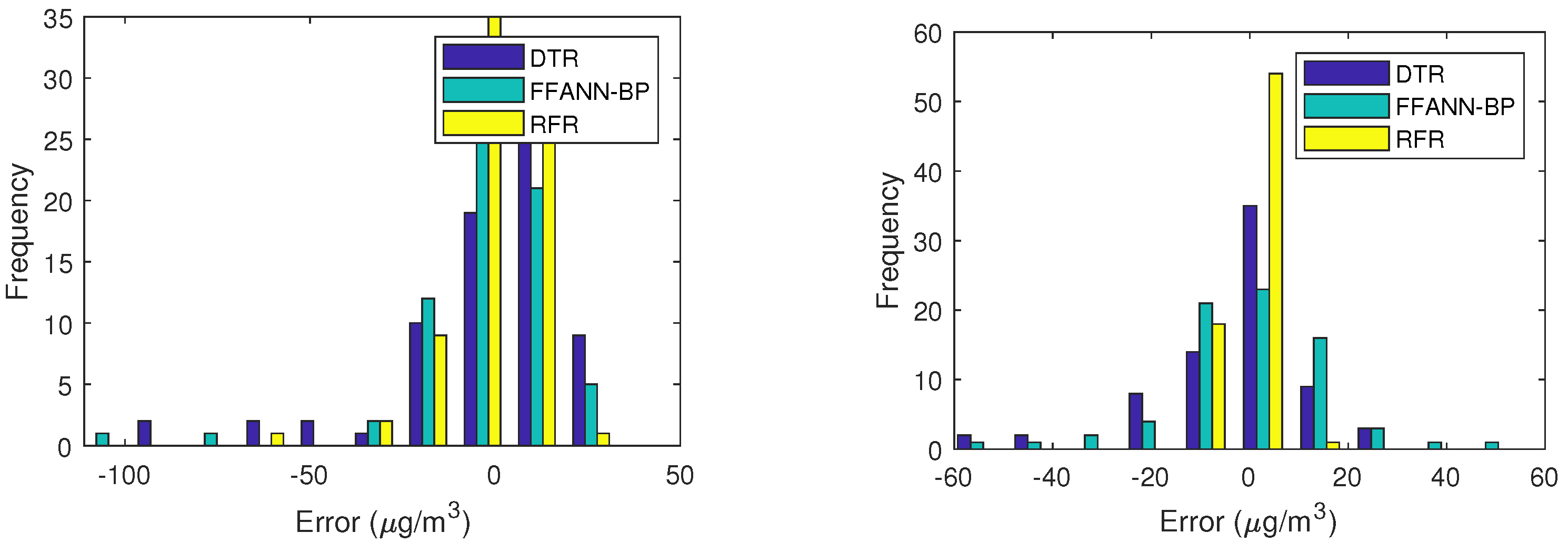
The time series plot of the ground measured air pollutant concentrations and the predictions by DTR, FFANN-BP and RFR are shown in Figure 7, Figure 8 and Figure 9. It can be observed that there is a higher agreement between the observed and predicted data. It is also shown that the predicted concentrations of RFR are closer to the observed data than those of the DTR and FFANN-BP, meaning that the RFR improves the predicted performance of air pollutant concentrations. We also employ the histograms to provide further insight into the relationship of the predictors with air pollutant concentrations in Figure 10, Figure 11 and Figure 12. RFR for air pollutant concentrations is very good since the histogram of RMSE is very steep and it is also considerable for the other pollutants in Figure 10, Figure 11 and Figure 12. At the same time, according to the construction time of the models, RMSE, MAE, MAPE are analyzed to evaluate the model. The prediction accuracy and model construction efficiency of different machine learning models are compared and analyzed. Appropriate variables are selected for the prediction of air pollutant concentrations. In terms of prediction accuracy, the RFR model has the best prediction ability, followed by the FFANN-BP model, and the DTR model. RFRs have stable accuracy and good prediction capability. The results show that RFR not only increases the performance of the prediction of air pollutant concentrations in Ningxia, but also discriminates the influential factors and reduces the dimension of the data, therefore reduces the time complexity of the algorithm.

RFR uses the average reduction of node impurity to describe the importance of the variables. The greater the reduction of node impurity by a factor, the more important the factor becomes. The importance of variables in the decision tree model is measured in the form of weight. The greater the weight of a factor, the stronger the influence of the factor in affecting the concentration of air pollutants. In this research, the importance of each factor on the prediction of air pollutant concentration is further analyzed. Figure 13, Figure 14 and Figure 15 and

Table 7. The importances of influential factor at Ma Lian Kou in 2016.

Pollutants	Index	Mean GST	Mean RHU	SSD	${\mathit{NO}}_2$	${\mathit{O}}_3$	${\mathit{PM}}_{2.5}$	${\mathit{PM}}_{10}$
CO	DTR	0.01	0.0	0.0	0.99
	RFR	0.16	0.1	0.12	0.63
$N{O}_2$	DTR	0.19	0.12	0.07		0.08		0.55
	RFR	0.19	0.08	0.06		0.09		0.58
$O_3$	DTR	0.61	0.14	0.07	0.09			0.1
	RFR	0.64	0.14	0.07	0.08			0.08
$P{M}_{2.5}$	DTR	0.03	0.04	0.03	0.33	0.01		0.57
	RFR	0.03	0.1	0.03	0.24	0.02		0.58
$P{M}_{10}$	DTR	0.02	0.02	0.02	0.16	0.05	0.73
	RFR	0.03	0.04	0.03	0.19	0.02	0.69
$S{O}_2$	DTR	0.17	0.06	0.05	0.66	0.04	0.03
	RFR	0.16	0.05	0.03	0.69	0.04	0.03

Mean GST, Mean RHU and SSD represent the average ground surface temperature, average relative humidity and sun shine duration, respectively.

show the analysis of the most important features of DTR and RFR for six air pollutant at Ma Lian Kou. The characteristic variables considered include meteorological factors, air pollutant concentrations of the previous day.

For $CO$, it can be seen that the concentrations of $N{O}_2$ rank first and contribute the most. For $N{O}_2$, it can be seen that $P{M}_{10}$ concentrations rank first and contribute the most. For $O_3$, it can be seen that ground surface temperature ranks first and contributes the most. For $S{O}_2$, it can be seen that $N{O}_2$ concentration ranks first and contributes the most. For $P{M}_{2.5}$, it can be seen that $P{M}_{10}$ concentration ranks first and contributes the most. For $P{M}_{10}$, it can be seen that $P{M}_{2.5}$ concentration ranks first and contributes the most. As shown in Table 5, the weight importance of temperature, relative humidity and air pressure are 14 and 25 in turn, indicating that ground surface temperature and relative humidity have the greatest impact on the concentration of air pollutants predicted by DTR, followed by air pressure and precipitation, and wind speed has the least impact. Figure 13, Figure 14 and Figure 15 and Table 7 shows the importance analysis of various influencing factors when we use decision tree and random forest algorithm to predict the concentration of various air pollutants in 2016. As shown in Figure 13, Figure 14 and Figure 15 and Table 7, for CO, $N{O}_2$ is the most important factors in both methods. For $N{O}_2$, $P{M}_{10}$ is the most important factor. For ozone, the ground surface temperature is the most important factor. $P{M}_{2.5}$ and $P{M}_{10}$ are the most important influencing factors for each other. $N{O}_2$ is the most important factor in the prediction of $S{O}_2$.

Table 8. The runtime of the three algorithm at Ma Lian Kou in 2016, all in (s).

	FFANN-BP	DTR	RFR
$CO$	0.058	0.002	0.032
$N{O}_2$	0.242	0.002	0.034
$O_3$	0.303	0.002	0.034
$P{M}_{2.5}$	0.349	0.002	0.04
$P{M}_{10}$	0.206	0.002	0.038
$S{O}_2$	0.364	0.002	0.038

shows the running time of the three algorithms on the concentrations of six pollutants in Ma Lian Kou in 2016. It can be seen from the Table 8 that the running time of DTR is the shortest due to its simple structure, FFANN-BP model takes the longest time to build, followed by RFR model. The running time of RFR is much lower than that of FFANN-BP. This is enough to reflect that RFR has low time complexity.

Due to the randomness of the three methods, the accuracy of the three methods cannot be evaluated by one experimental result. Therefore, this paper runs 1000 Monte Carlo experiments and takes the average of the running results to evaluate the accuracy of the three methods. The results in

Table 9. The mean, variance and the confidence interval of the predicted concentrations for six air pollutants based on 1000 Monte Carlo experiments at Ma Lian Kou in 2016.

	Mean	Variance	${\mathit{CI}}_{\mathit{l}}$	${\mathit{CI}}_{\mathit{u}}$
$CO$	0.65	0.14	0.42	0.85
$N{O}_2$	4.4	0.73	3.1	6.8
$O_3$	85.8	11.7	60.7	100.9
$P{M}_{2.5}$	33.9	8.5	28.8	34.1
$P{M}_{10}$	135.9	22.8	91.8	156.9
$S{O}_2$	1.9	0.8	1.2	6.6

show that the accuracy and prediction stability of RFR are better than the other two methods.

The performances achieved highlight that for the extreme concentrations of air pollutants, the performance of the DTR is not significant. The reason is that the construction project of this period is particularly high in Ningxia. However, RFR still acceptedly performs even with the sudden occurrence of such event. For the particulate matter, we find the decrease in performance of DTR and FFANN-BP, making the variance of the concentrations of the particulate matter larger. However, RFR is still more adaptable than FFANN-BP and DTR. It shows that the DTR model has poor prediction ability in using the meteorological elements to predict air pollutant concentrations, and it is recommended to use the RFR model to predict air pollutant concentrations.

5. Conclusions

In this study, Ningxia Province, where air pollution has been increasing in recent years, is selected as the research area. It is shown that the concentrations of $CO$, $P{M}_{10}$ and $P{M}_{2.5}$ were higher in the cold and dry winter than those in summer because of the combustion of fossil fuels for heating purposes. The aim of this study was to propose a modelling procedure that would yield satisfactory results for the prediction of ambient air pollutant concentrations. In this work DT, FFANN-BP and RFR models were proposed for predicting the air pollutant concentrations in Ningxia, China. The levels of air pollutant concentrations were observed in three air monitoring stations, the capital of Ningxia and the rural areas of Ningxia.

The collected data for air pollutant concentrations and meteorological variables were used for the development of DTR, FFANN-BP and RFR. Data was prepared by calculating the average of the air pollutant concentrations for each day of the study period. Compared with DTR and FFANN-BP, it is evident that RFR is superior to the other methods. Furthermore, the proposed method has been successfully applied to the analysis of the importance of the predictors. We conducted an uncertainty analysis based on Monte Carlo experiments. The proposed method has worked well in predicting the air pollutant concentrations and can be effectively utilized for the analysis of the importance of the predictors. It reveals that there is a close relationship between air pollutant concentrations and meteorological variables. Hence, the developed model is capable of generating better forecasting performance for air pollutant concentrations. Because of the generality of the algorithm, it can be applied to other area and databases.

It can be incorporated into the control and management for a cleaner air and a better environment in many cities. Furthermore, we will consider other ways of using the spatial and meteorological conceptions. Our future research work will focus on the improvement and optimization of machine learning models. Multimodal analysis can effectively decompose the time periodic change trend and noise of air pollutant concentration. Therefore, the introduction of multimodal analysis into random forest regression model can effectively improve the prediction accuracy and the prediction of air pollutant concentration in extreme pollution weather, which will be a problem to be solved in the future.

References

1. Berg, A.; McColl, K.A. No projected global dry lands expansion under greenhouse warming. Nat. Clim. Chang. 2021, 11, 331–337. [Google Scholar] [CrossRef]
2. Liao, Z.; Gao, M.; Sun, J.; Fan, S. The impact of synoptic circulation on air quality and pollution-related human health in the Yangtze River Delta region. Sci. Total Environ. 2017, 607, 838–846. [Google Scholar] [CrossRef]
3. Pang, Y.; Huang, W.; Luo, X.; Chen, Q.; Zhan, Z.; Tang, M.; Hong, Y.; Chen, J.; Li, H. In-vitro human lung cell injuries induced by urban PM2.5 during a severe air pollution episode: Variations associated with particle components. Ecotoxicol. Environ. Saf. 2020, 206, 111406. [Google Scholar] [CrossRef]
4. Shang, Y.; Sun, Z.; Cao, J.; Wang, X.; Zhong, L.; Bi, X.; Li, H.; Liu, W.; Zhu, T.; Huang, W. Systematic review of Chinese studies of short-term exposure to air pollution and daily mortality. Environ. Int. 2013, 54, 100–111. [Google Scholar] [CrossRef]
5. Shaddick, G.; Thomas, M.L.; Amini, H. Data integration for the assessment of population exposure to ambient air pollution for global burden of disease assessment. Environ. Sci. Technol. 2018, 52, 9069–9078. [Google Scholar] [CrossRef]
6. Zhang, J.S.; Ding, W.F. Prediction of air pollutants concentration based on extreme learning machine: The case of Hong Kong. Int. J. Environ. Sci. Public Health 2017, 7, 114. [Google Scholar] [CrossRef]
7. Dennis, R.L.; Byun, D.W.; Novak, J.H. The next generation of integrated air quality modeling: EPA’s models-3. Atmos. Environ. 1996, 30, 1925–1938. [Google Scholar] [CrossRef]
8. Wang, Z.F.; Xie, F.Y.; Wang, X.Q. Development and application of nested air quality prediction modeling system. Atmos. Sci. 2006, 31, 778–790. [Google Scholar]
9. Batterman, S.A.; Zhang, K.; Kononowech, R. Prediction and analysis of near-road concentrations using a reduced-form emission/dispersion model. Environ. Health 2010, 9, 29. [Google Scholar] [CrossRef] [Green Version]
10. Abal, G.; Aicardi, D.; Suarez, R.A.; Laguarda, A. Performance of empirical models for diffuse fraction in uruguay. Sol. Energy 2017, 141, 166–181. [Google Scholar] [CrossRef]
11. Briant, R.; Seigneur, C.; Gadrat, M.; Bugajny, C. Evaluation of roadway gaussian plume models with large- scale measurement campaigns. Geosci. Model. 2013, 6, 445–456. [Google Scholar] [CrossRef] [Green Version]
12. Mishra, D.; Goyal, P. Development of artificial intelligence based NO2 forecasting models at Taj Mahal, Agra centre for atmospheric sciences. Atmos. Pollut. Res. 2015, 6, 99–106. [Google Scholar] [CrossRef] [Green Version]
13. Pahlavani, P.; Sheikhian, H.; Bigdeli, B. Assessment of an air pollution monitoring network to generate urban air pollution maps using Shannon information index, fuzzy overlay, and Dempster-Shafer theory, A case study: Tehran, Iran. Atmos. Environ. 2017, 167, 254–269. [Google Scholar] [CrossRef]
14. Sayegh, A.S.; Munir, S.; Habeebullah, T.M. Comparing the performance of statistical models for predicting PM10 concentrations. Aerosol. Air Qual. Res. 2014, 14, 653–665. [Google Scholar] [CrossRef] [Green Version]
15. Chen, Y.; Zheng, W.; Li, W.; Huang, Y. Large group activity security risk assessment and risk early warning based on random forest algorithm. Pattern Recognit. Lett. 2021, 144, 1–5. [Google Scholar] [CrossRef]
16. Danesh Yazdi, M.; Kuang, Z.; Dimakopoulou, K.; Barratt, B.; Suel, E.; Amini, H.; Schwartz, J. Predicting fine particulate matter (PM2.5) in the greater London area: An ensemble approach using machine learning methods. Remote Sens. 2020, 12, 914. [Google Scholar] [CrossRef] [Green Version]
17. Ding, W.F.; Zhang, J.S. Prediction of air pollutant concentration based on sparse response backpropagation training feedforward neural networks. Environ. Sci. Pollut. Res. 2016, 23, 19481–19494. [Google Scholar] [CrossRef]
18. Ding, W.; Leung, Y.; Zhang, J.; Fung, T. A hierarchical Bayesian model for the analysis of space-time air pollutant concentrations and an application to air pollution analysis in Northern China. Stoch. Environ. Res. Risk Assess. 2021, 35, 2237–2271. [Google Scholar] [CrossRef]
19. Joharestani, M.Z.; Cao, C.; Ni, X.; Bashir, B.; Talebiesfandarani, S. PM2.5 Prediction based on random forest, XGBoost, and deep learning using multisource remote sensing data. Atmosphere 2019, 10, 373. [Google Scholar] [CrossRef] [Green Version]
20. Sanchez, A.B.; Ordóñez, C.; Lasheras, F.S.; de Cos Juez, F.J.; Roca-Pardias, J. Forecasting SO2 pollution incidents by means of elman artificial neural networks and ARIMA models. In Abstract and Applied Analysis; Hindawi: London, UK, 2013; pp. 1–6. [Google Scholar]
21. Li, L.; Zhang, J.; Qiu, W.; Wang, J.; Fang, Y. An ensemble spatiotemporal model for predicting PM2.5 concentrations. Int. J. Environ. Res. Public Health 2017, 14, 549. [Google Scholar] [CrossRef] [Green Version]
22. Liu, N.; Zou, B.; Li, S.; Zhang, H.; Qin, K. Prediction of PM2.5 concentrations at unsampled points using multiscale geographically and temporally weighted regression. Environ. Pollut. 2021, 284, 117116. [Google Scholar] [CrossRef]
23. Alimissis, A.; Philippopoulos, K.; Tzanis C, G. Spatial estimation of urban air pollution with the use of artificial neural network models. Atmos. Environ. 2018, 191, 205–213. [Google Scholar] [CrossRef]
24. Bahari, R.A.; Abbaspour, R.A.; Pahlavani, P. Prediction of PM2.5 concentrations using temperature inversion effects based on an artificial neural network. In Proceedings of the ISPRS International Conference of Geospatial Information Research, Tehran, Iran, 15–17 November 2014; Volume 15, p. 17. [Google Scholar]
25. Feng, X.; Li, Q.; Zhu, Y.; Hou, J.; Jin, L.; Wang, J. Artificial neural networks forecasting of PM2.5 pollution using air mass trajectory based geographic model and wavelet transformation. Atmos. Environ. 2015, 107, 118–128. [Google Scholar] [CrossRef]
26. Valentini, G. Ensemble Methods: A Review, in Advances in Machine Learning and Data Mining for Astronomy; Chapman & Hall Data Mining and Knowledge Discovery Series; CRC Press: London, UK, 2012; Volume 26, pp. 563–594. [Google Scholar]
27. Calkins, C.; Ge, C.; Wang, J.; Anderson, M.; Yang, K. Effects of meteorological conditions on sulfur dioxide air pollution in the North China plain during winters of 2006–2015. Atmos. Environ. 2016, 147, 296–309. [Google Scholar] [CrossRef]
28. Harishkumar, K.; Yogesh, K.; Gad, I. Forecasting air pollution particulate matter (PM2.5) using machine learning regression models. Procedia Comput. Sci. 2020, 171, 2057–2066. [Google Scholar]
29. Tobler, W.R. A Computer Movie Simulating Urban Growth in the Detroit Region. Econ. Geogr. 1970, 46 (Suppl. 1), 234–240. [Google Scholar] [CrossRef]
30. Ningxia Government. Overview of Ningxia. Available online: cn.nxcan.com/index.php?case=archive&act=show&aid=55 (accessed on 6 July 2015).
31. Ningxia Government. Ningxia Meteorology. Available online: https://sthjt.nx.gov.cn (accessed on 8 August 2014).
32. Sergey, I.; Christian, S. Batch normalization: Accelerating deep network training by reducing internal covariate shift. In Proceedings of the 32nd International Conference on Machine Learning, Lille, France, 6–11 July 2015; pp. 448–456. [Google Scholar]
33. Bishop, C. Neural Networks for Pattern Recognition, 3rd ed.; Oxford University Press: Oxford, UK, 1995. [Google Scholar]
34. Scikit-Learn: Machine Learning in Python. Available online: https://scikit-learn.org/stable/ (accessed on 9 September 2016).
35. Hastie, T.; Tibshirani, R.; Friedman, J. The elements of statistical learning. J. R. Stat. Soc. 2004, 167, 192. [Google Scholar]
Figure 1. The architecture of the FFANN-BP.
Atmosphere 13 00960 g001
Figure 2. The locations of air monitoring and meteorological stations, where the purple and blue solid point represent the air monitoring stations and meteorological stations in Ningxia, respectively.
Atmosphere 13 00960 g002
Figure 3. The variations of the concentrations for C O and N O 2 at Ma Lian Kou, Sha Po Tou and Ma Yuan in 2016.
Atmosphere 13 00960 g003
Figure 4. The variations of the concentrations for O 3 and S O 2 at Ma Lian Kou, Sha Po Tou and Ma Yuan in 2016.
Atmosphere 13 00960 g004
Figure 5. The variations of the concentrations for P M 2.5 and P M 10 at Ma Lian Kou, Sha Po Tou and Ma Yuan in 2016.
Atmosphere 13 00960 g005
Figure 6. The flowchart of our method.
Atmosphere 13 00960 g006
Figure 7. The observed concentrations and the predicted concentrations of DTR, FFANN-BP and RFR for C O and N O 2 at Ma Lian Kou, where the red line and the black, green and lightcyan lines represent the observations, and the predictions of DTR, FFANN-BP and RFR, respectively.
Atmosphere 13 00960 g007
Figure 8. The observed concentrations and the predicted concentrations of DTR, FFANN-BP and RFR for O 3 and S O 2 at Ma Lian Kou, where the red line and the black, green and lightcyan lines represent the observations, and the predictions of DTR, FFANN-BP and RFR, respectively.
Atmosphere 13 00960 g008
Figure 9. The observed concentrations and the predicted concentrations of DTR, FFANN-BP and RFR for P M 2.5 and P M 10 at Ma Lian Kou, where the red line and the black, green and lightcyan lines represent the observations, and the predictions of DTR, FFANN-BP and RFR, respectively.
Atmosphere 13 00960 g009
Figure 10. The error histogram of the prediction for C O and N O 2 at Ma Lian Kou.
Atmosphere 13 00960 g010
Figure 11. The error histogram of the prediction for O 3 and S O 2 at Ma Lian Kou.
Atmosphere 13 00960 g011
Figure 12. The error histogram of the prediction for P M 2.5 and P M 10 at Ma Lian Kou.
Atmosphere 13 00960 g012
Figure 13. The importance of predictor variables of RFR for (a) C O and (b) N O 2 at Ma Lian Kou.
Atmosphere 13 00960 g013
Figure 14. The importance of predictor variables of RFR for (a) O 3 and (b) S O 2 at Ma Lian Kou.
Atmosphere 13 00960 g014
Figure 15. The importance of predictor variables of RFR for (a) P M 2.5 and (b) P M 10 at Ma Lian Kou.
Atmosphere 13 00960 g015