Uncertainty Quantification of WRF Model for Rainfall Prediction over the Sichuan Basin, China

Abstract

The mesoscale Weather Research and Forecasting (WRF) model has been widely employed to forecast day-ahead rainfalls. However, the deterministic predictions from the WRF model incorporate relatively large errors due to numerical discretization, inaccuracies in initial/boundary conditions and parameterizations, etc. Among them, the uncertainties in parameterization schemes have a huge impact on the forecasting skill of rainfalls, especially over the Sichuan Basin which is located east of the Tibetan Plateau in southwestern China. To figure out the impact of various parameterization schemes and their interactions on rainfall predictions over the Sichuan Basin, the Global Forecast System data are chosen as the initial/boundary conditions for the WRF model and 48 ensemble tests have been conducted based on different combinations of four microphysical (MP) schemes, four planetary boundary layer (PBL) schemes, and three cumulus (CU) schemes, for four rainfall cases in summer. Compared to the observations obtained from the Chinese ground-based and encrypted stations, it is found that the Goddard MP scheme together with the asymmetric convective model version 2 PBL scheme outperforms other combinations. Next, as the first step to explore further improvement of the WRF physical schemes, the polynomial chaos expansion (PCE) approach is then adopted to quantify the impacts of several empirical parameters with uncertainties in the WRF Single Moment 6-class (WSM6) MP scheme, the Yonsei University (YSU) PBL scheme and the Kain-Fritsch CU scheme on WRF rainfall predictions. The PCE statistics show that the uncertainty of the scaling factor applied to ice fall velocity in the WSM6 scheme and the profile shape exponent in the YSU scheme affects more dominantly the rainfall predictions in comparison with other parameters, which sheds a light on the importance of these schemes for the rainfall predictions over the Sichuan Basin and suggests the next step to further improve the physical schemes.

1. Introduction

The frequency of natural disasters that occur due to extreme rainfalls is increasing these days [1,2,3]. Extreme rainfalls can cause widespread devastation, such as floods and landslides, resulting in loss of life and personal property damage. Therefore, accurate rainfall prediction is of great importance to take preventive measures.

Short-term rainfall prediction relies on mesoscale numerical weather prediction (NWP) models. Although a number of works have been done to develop NWP models, there exists a significant amount of uncertainty associated with initial/boundary conditions, discretizations and physical parameterizations, etc., which still limits the accuracy of NWP models. Through assimilating quality-controlled observations [4,5] and adopting advanced numerical discretization methods [6], the prediction of the NWP model can be highly improved. In addition, the study of physical parameterization also has significant impact on the NWP model’s forecasts. For example, a multi-physics ensemble method using different parameterization schemes was employed to study a Mediterranean cyclone [7]. Evans et al. [8] simulated four East Coast Lows events using the weather research and forecasting (WRF) model with 36 model configurations and found that the combination of the Mellor-Yamada-Janjic (MYJ) planetary boundary layer (PBL) and the Betts-Miller-Janjic (BMJ) cumulus (CU) scheme can substantially improve the simulation of heavy rainfall. Another study [9] showed that the scheme combination of the WRF Single Moment 3-class (WSM3) and the Grell-Devenyi (GD) ensemble had a robust performance in leveraging the prediction ability and computational efficiency of the prediction of heavy precipitation. Liu et al. [10] found that the best model configuration for extreme rainfall events over Egypt consisted of the WRF Single Moment 6-class (WSM6) microphysical (MP), the MYJ PBL and the Grell-Freitas CU schemes. Whereas, the combination of WSM6 and Kain-Fritsch (KF) schemes performed optimally in the rainfall forecasts over the Hanjiang River Basin in China [11]. These studies proved that physical parameterization schemes have different performances in different study regions and no identical model configuration for all areas. The multi-physics ensemble can be a solution for determining optimal physics configuration to some extent in a study area of interest.

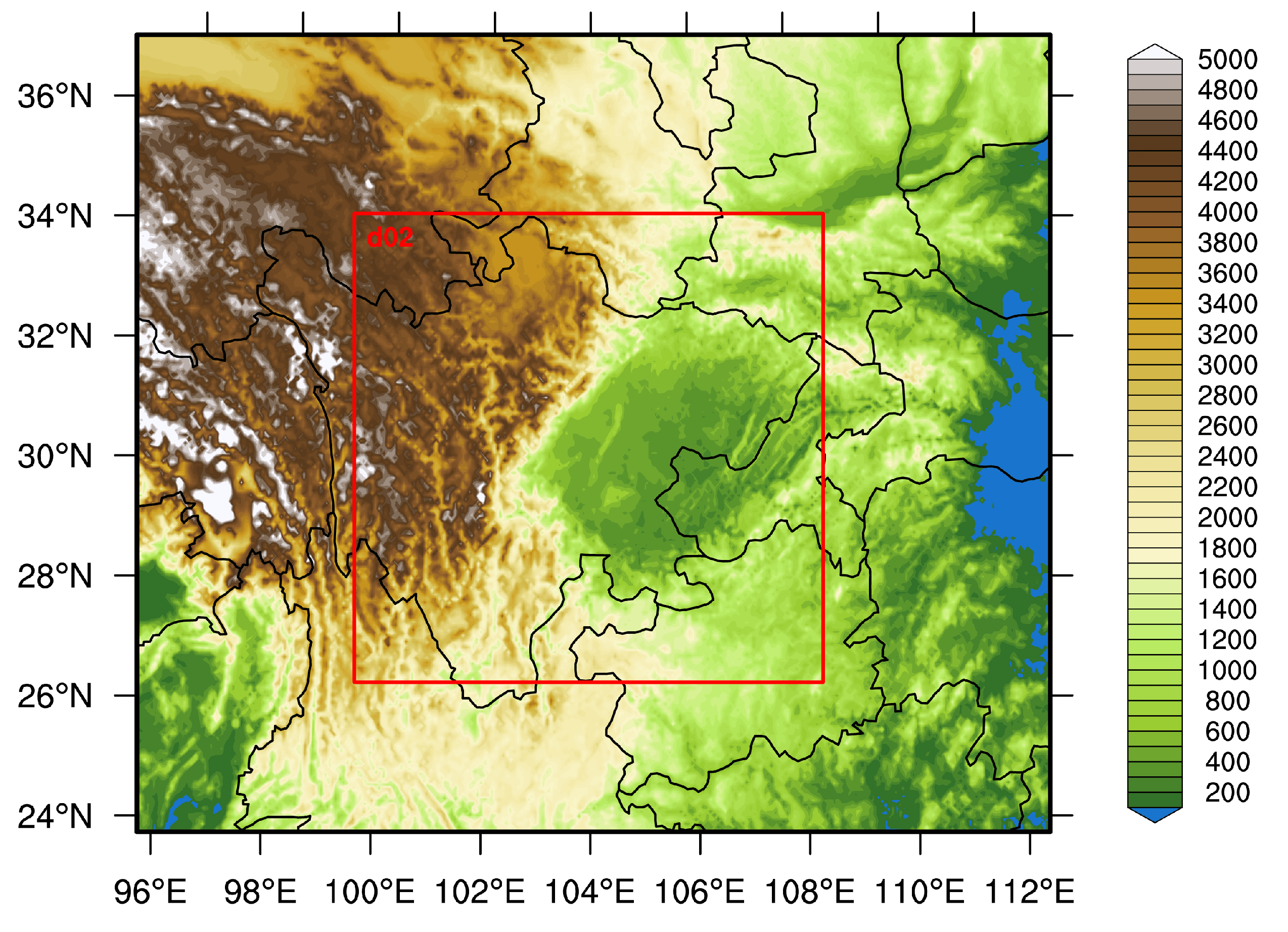
The focus of this paper is on the Sichuan Basin (shown in Figure 1), which is an expansive 229,500 km² low-land region surrounded by the highlands of the Tibetan Plateau on the west, the Daba Mountains on the north, the Wu Mountains on the east, and the Yunnan-Guizhou Plateau on the south. Its unique characteristics of geographical location and complex terrain, especially on the western side of the basin, lead to more significant difficulties in simulating rainfall events than other areas with simple topography. Several prior studies [12,13] have focused on revealing the impact of basin terrains on PBL due to its vital role in the interaction of the earth-atmosphere system. The station observation and reanalysis data have been analyzed to show the atmosphere’s PBL processes and vertical structure over basin terrains [12]. Besides, WRF model was employed to examine the performance of different PBL and MP schemes in the rainfall prediction over the Sichuan Basin. The literature also reported that the impact of cumulus schemes on rainfall forecast of WRF model in Sichuan is of great importance [14].

Nonetheless, we consider that the literature regarding uncertainties brought by parameterization schemes to rainfall prediction over the Sichuan Basin is still limited, and it deserves further exploration. Most studies have not focused on the interaction of various physical schemes. Therefore, as this study’s first objective, we run 48 ensemble tests to comprehensively show the difference of multiple combinations of physical schemes in the WRF model on summer rainfall over the Sichuan Basin.

The other purpose of this study is to quantify the parametric uncertainty in the physical schemes related to rainfall forecasting. As known, one of the biggest challenges in sub-grid physics modeling is identifying the parameters [15,16]. The traditional approach assigns “most likely” values to those parameters from the corresponding ranges; however, such an approach can not be adequate in any cases as the complex physical processes may be sensitive to some of the parameters. For example, the different values of the critical Richardson number in the asymmetric convective model version 2 (ACM2) PBL scheme [17] and the coefficient for solving the ice crystal fall velocity in the WSM6 MP scheme [18] have large impact on the calculation of the boundary layer height and the accretion amount from ice to water, respectively. Nevertheless, quantifying the uncertainties originating from the empirical parameters in each physical package of the WRF model has not yet been paid much attention.

In the atmosphere field, one of the most common sampling methods used to implement sensitivity analysis is the Monte Carlo (MC) [19] approach or one of its variants [20,21]. Although MC sampling is straightforward to implement because it only requires repetitive executions of deterministic simulations, a very large number of resultant executions are needed to obtain reliable statistics such as mean value and standard deviation (STD) due to the relatively slow rate of convergence. More recently, other sampling methods such as full factorial [22] and Latin hypercube [23,24] have been employed for generating a near-random sample of parameter values. The Morris one-at-a-time (MOAT) [25] method was also applied to the NWP field [26] and it proved to be an effective method that can screen out the most sensitive parameter. As mentioned before, many of these approaches need a large number of realizations for accurate results, especially for the systems like an NWP model with large parameter counts, which can incur an excessive computational burden.

Many efforts have been made to reduce the computational burden in the field of uncertainty quantification (UQ) [27,28]. Polynomial approximation plays a vital role in the context of UQ. In recent years, the state-of-the-art polynomial chaos expansion (PCE) method [29] has been widely used to analyze and quantify the uncertainty caused by uncertain parameters in a system of interest [30,31]. It is a non-sampling method which represents the uncertain quantities as an expansion of orthogonal polynomials in terms of random variables. In contrast to most sampling methods (e.g., MC simulations), the computational costs of PCE are often significantly lower [32]. More detailed information of PCE can be found in Section 3.

Given these considerations, we present a framework based on the PCE method and WRF model to quantitatively analyze the impact of uncertain parameters in WRF parameterization schemes on rainfall prediction in the Sichuan Basin, as the second part of this work. Knowledge of the parameters with large uncertainties is of crucial importance to improve the forecasting skill of rainfall over the Sichuan Basin and shows the direction to further improve the physical schemes in the WRF model.

The main contributions of this paper are summarized as follows:

• The difference of multiple combinations of physical parameterization schemes of WRF model in summer rainfall prediction over the Sichuan Basin has been comprehensively examined.
• To the authors’ best knowledge, it is the first time that employing the advanced PCE method to study the parametric uncertainty in WRF rainfall prediction.
• We show that the PCE-WRF framework is able to identify the parameters with significant uncertainties in specific physical schemes. The results might show the direction to improve these physical schemes further.

The rest of this paper is organized as follows. The datasets, WRF model configuration, and multiple evaluation metrics are described in Section 2. Section 3 presents a brief introduction of PCE approach employed in this study. Section 4 presents and analyzes the main results and Section 5 contains the concluding remarks.

2. Data and Model

2.1. Data

Global-scale atmospheric datasets, such as Global Forecast System (GFS) data and ECMWF Reanalysis v5 (ERA5), are always used to drive the mesoscale models, refs. [33,34,35,36] have evaluated those existing large-scale datasets in terms of wind, rainfall, solar radiance, etc. In this study, we choose the GFS data as the initial/boundary conditions for the regional high-resolution WRF model. The data periods are consistent with the WRF model simulation periods with a 3-h interval, and a horizontal resolution of 0.25 × 0.25 degree for all variables. The topographic data is fetched from the U.S. Geological Survey (USGS) global 30 arc-s elevation (GTOPO30) dataset for nested domain.

Rainfall observations from approximately 9800 Chinese ground-based and encrypted stations over the Sichuan Basin (shown in Figure 2) are interpolated to the WRF model grid points to evaluate the WRF model’s output. The time interval is one hour. Besides, ERA5 hourly reanalysis data are adopted to show the weather systems and vapor condition of the rainfall cases selected in this study.

2.2. WRF Model Configuration and Ensemble Design

2.2.1. WRF Model Configuration

The high-resolution mesoscale meteorological model chosen in the study is the Weather Research and Forecasting (WRF) model with Advanced Research WRF (ARW) version 3.6.1. The forecasting domain is configured by following the recommendations in [37,38]. As shown in Figure 1, one parent and a nested domain (D02) with a horizontal resolution of 9 km (190 × 166 grid points) and 3 km (291 × 291 grid points), respectively, are chosen. There are 35 vertically stretched eta levels for the two domains, and the time step is 36 s. In this study, we run the WRF model on “cold-start” mode at 06:00 UTC each day, and each run lasts thirty hours. The first six hours are regarded as the spin-up period [39]. Model output has a constant interval of one hour.

The physical parameterization schemes adopted include the Dudhia shortwave radiation scheme [40], the Rapid Radiative Transfer Model long-wave radiation scheme [41], and the Noah land surface model [42]. The configuration of MP, PBL and CU schemes can be found in Section 2.2.2.

2.2.2. Multi-Physics Ensemble

For the sake of quantifying the uncertainty and improving the accuracy of the WRF model on precipitation simulations over the Sichuan Basin, we evaluate the performance of different physical options. The rainfall prediction highly related three parameterization schemes, i.e., MP, PBL, and CU schemes, are employed to generate ensemble members (as summarized in

Table 1. Parameterization scheme combinations used to create ensemble members. The numbers in parentheses represent the physics options in WRF model.

Ensemble Member	MP	PBL/Surface Layer	CU
M1	Lin et al. (2)	YSU (1)/MM5 similarity (1)	KF (1)
M2	Lin et al. (2)	YSU (1)/MM5 similarity (1)	BMJ (2)
M3	Lin et al. (2)	YSU (1)/MM5 similarity (1)	GD (3)
M4	Lin et al. (2)	MYJ (2)/Eta similarity (2)	KF (1)
M5	Lin et al. (2)	MYJ (2)/Eta similarity (2)	BMJ (2)
M6	Lin et al. (2)	MYJ (2)/Eta similarity (2)	GD (3)
M7	Lin et al. (2)	QNSE (4)/QNSE (4)	KF (1)
M8	Lin et al. (2)	QNSE (4)/QNSE (4)	BMJ (2)
M9	Lin et al. (2)	QNSE (4)/QNSE (4)	GD (3)
M10	Lin et al. (2)	ACM2 (7)/MM5 similarity (1)	KF (1)
M11	Lin et al. (2)	ACM2 (7)/MM5 similarity (1)	BMJ (2)
M12	Lin et al. (2)	ACM2 (7)/MM5 similarity (1)	GD (3)
M13	WSM6 (6)	YSU (1)/MM5 similarity (1)	KF (1)
M14	WSM6 (6)	YSU (1)/MM5 similarity (1)	BMJ (2)
M15	WSM6 (6)	YSU (1)/MM5 similarity (1)	GD (3)
M16	WSM6 (6)	MYJ (2)/Eta similarity (2)	KF (1)
M17	WSM6 (6)	MYJ (2)/Eta similarity (2)	BMJ (2)
M18	WSM6 (6)	MYJ (2)/Eta similarity (2)	GD (3)
M19	WSM6 (6)	QNSE (4)/QNSE (4)	KF (1)
M20	WSM6 (6)	QNSE (4)/QNSE (4)	BMJ (2)
M21	WSM6 (6)	QNSE (4)/QNSE (4)	GD (3)
M22	WSM6 (6)	ACM2 (7)/MM5 similarity (1)	KF (1)
M23	WSM6 (6)	ACM2 (7)/MM5 similarity (1)	BMJ (2)
M24	WSM6 (6)	ACM2 (7)/MM5 similarity (1)	GD (3)
M25	Goddard (7)	YSU (1)/MM5 similarity (1)	KF (1)
M26	Goddard (7)	YSU (1)/MM5 similarity (1)	BMJ (2)
M27	Goddard (7)	YSU (1)/MM5 similarity (1)	GD (3)
M28	Goddard (7)	MYJ (2)/Eta similarity (2)	KF (1)
M29	Goddard (7)	MYJ (2)/Eta similarity (2)	BMJ (2)
M30	Goddard (7)	MYJ (2)/Eta similarity (2)	GD (3)
M31	Goddard (7)	QNSE (4)/QNSE (4)	KF (1)
M32	Goddard (7)	QNSE (4)/QNSE (4)	BMJ (2)
M33	Goddard (7)	QNSE (4)/QNSE (4)	GD (3)
M34	Goddard (7)	ACM2 (7)/MM5 similarity (1)	KF (1)
M35	Goddard (7)	ACM2 (7)/MM5 similarity (1)	BMJ (2)
M36	Goddard (7)	ACM2 (7)/MM5 similarity (1)	GD (3)
M37	Thompson (8)	YSU (1)/MM5 similarity (1)	KF (1)
M38	Thompson (8)	YSU (1)/MM5 similarity (1)	BMJ (2)
M39	Thompson (8)	YSU (1)/MM5 similarity (1)	GD (3)
M40	Thompson (8)	MYJ (2)/Eta similarity (2)	KF (1)
M41	Thompson (8)	MYJ (2)/Eta similarity (2)	BMJ (2)
M42	Thompson (8)	MYJ (2)/Eta similarity (2)	GD (3)
M43	Thompson (8)	QNSE (4)/QNSE (4)	KF (1)
M44	Thompson (8)	QNSE (4)/QNSE (4)	BMJ (2)
M45	Thompson (8)	QNSE (4)/QNSE (4)	GD (3)
M46	Thompson (8)	ACM2 (7)/MM5 similarity (1)	KF (1)
M47	Thompson (8)	ACM2 (7)/MM5 similarity (1)	BMJ (2)
M48	Thompson (8)	ACM2 (7)/MM5 similarity (1)	GD (3)

). The MP scheme mainly involves the processes of explicitly resolved water vapor, cloud, and precipitation. In this paper, we use four different MP schemes including the Lin scheme [43], WSM6 scheme [44], Goddard scheme [45], and Thompson scheme [46]. Despite the differences in ice phase processes, these schemes all include snow, graupel, and ice processes and are appropriate for high-resolution simulations. For the PBL process which is closely related to the spatial distribution of precipitation, the Yonsei University (YSU) PBL scheme [47], the MYJ PBL scheme [48], the Quasi-Normal Scale Elimination (QNSE) PBL scheme [49], and the ACM2 PBL scheme [50] are chosen. We also choose three CU schemes, i.e., the Kain-Fritsch (KF) scheme [51], the BMJ scheme [48] and the GD scheme [52], which can detail the convective component of rainfall and predominate the estimate of precipitation rate. It should be noted that CU parameterization schemes are not used in the nested domain with a resolution of 3 km because CU parameterization is theoretically only valid for a coarser grid size (e.g., greater than 5 km) [53].

2.3. Evaluation Metrics

The global metrics used for comparison between ensembles are the root mean square error (RMSE), the mean absolute error (MAE) and the correlation coefficient (CC), defined as:

$$RMSE=\sqrt{\frac{1}{N}\sum _{i=1}^N{\left({R_f}_i-{R_o}_i\right)}^2},$$

(1)

$$MAE=\frac{1}{N}\sum _{i=1}^N|{R_f}_i-{R_o}_i|,$$

(2)

$$CC=\frac{{\sum }_{i=1}^N\left({R_f}_i-\overline{R_f}\right)\left({R_o}_i-\overline{R_o}\right)}{\sqrt{{\sum }_{i=1}^N{\left({R_f}_i-\overline{R_f}\right)}^2{\sum }_{i=1}^N{\left({R_o}_i-\overline{R_o}\right)}^2}},$$

(3)

where i is the grid point and N is the total number of verification points. $R_f$ and $R_o$ denote the rainfall forecasts and the corresponding observations, respectively.

Besides, we utilize the structure-amplitude-location (SAL) [54] index to quantitatively and comprehensively evaluate WRF model’s rainfall forecasts. The three components of SAL are defined as follows,

$$\begin{array}{cc}\hfill & S=\frac{V\left(R_f\right)-V\left(R_o\right)}{0.5\left[V\left(R_f\right)+V\left(R_o\right)\right]},\hfill \end{array}$$

(4)

$$A=\frac{D\left(R_f\right)-D\left(R_o\right)}{0.5[D\left(R_f\right)+D\left(R_o\right)]},$$

(5)

$$L=L_1+L_2=\frac{|\mathbf{x}\left(R_f\right)-\mathbf{x}\left(R_o\right)|}{d}+\frac{2|\mathbf{r}\left(R_f\right)-\mathbf{r}\left(R_o\right)|}{d},$$

(6)

where $V\left(R\right)=\left({\sum }_{n=1}^M{R}_n{V}_n\right)/\left({\sum }_{n=1}^M{R}_n\right)$, $V_n=R_n/R_n^{max}$ is the scaled precipitation volume of object n, and M denotes the total number of precipitation objects in the domain. The domain average of rainfall $D\left(R\right)=\frac{1}{N}{\sum }_{\left(i,j\right)\in D}{R}_{\left(i,j\right)}$. In Equation (6), $\mathbf{x}\left(R\right)$ denotes the center of mass of the precipitation field, $\mathbf{r}\left(R\right)=({\sum }_{n=1}^M{R}_n|\mathbf{x}-{\mathbf{x}}_n\left|\right)/{\sum }_{n=1}^M{R}_n$, and d is the largest distance between two boundary points of the domain. Therefore, $L_1$ is the normalized distance between the two centers of mass of the predicted and observed precipitation bodies while $L_2$ is the average distance of the center of mass between the total precipitation fields and each precipitation individual objects. Perfect rainfall forecasts are characterized by zero values for all three components of SAL.

Finally, the equitable threat score (ETS) being a metric that measures the skill of a precipitation forecast relative to chance is also used in the present study to evaluate the ability of an NWP model for predicting precipitation that falls into different threshold ranges (

Table 2. Grading of precipitation intensity.

Grade	Precipitation in 12 h (mm)	Precipitation in 24 h (mm)
Light rain	[0.1, 5)	[0.1, 10.0)
Moderate rain	[5, 15)	[10.0, 25.0)
Heavy rain	[15, 30)	[25.0, 50.0)
Storm	[30, 70)	[50.0, 100.0)
Heavy storm	[70, 140)	[100.0, 250.0)

), defined as:

$$\begin{array}{cc}\hfill ETS& =\frac{A-A_r}{A+B+C-A_r}\hfill \\ \hfill A_r& =\frac{(A+B)(A+C)}{A+B+C+D}\hfill \end{array},$$

(7)

where A, B, C, and D stand for hits (events forecast to occur, and did occur), false alarms (events forecast to occur, but did not occur), missing (events forecast not to occur, but did occur), and correct negatives (event forecast not to occur, and did not occur), respectively. Generally, the range of ETS is from $-\frac{1}{3}$ to 1, and 1 is the perfect score.

3. Uncertainty Quantification Method

As mentioned earlier, there are many uncertainties in the WRF models’ physical parameterization schemes. Some of the parameters with uncertainties in these schemes might affect the rainfall forecasts significantly. We therefore employ the PCE approach to quantitatively assess those uncertainties. In this section, we give a brief introduction of PCE method used in this study.

3.1. PCE Approach

Generally, the PCE approach formulates the relationship between the system output $y\left(\xi \right)$ and each random input $\xi$ using a series of orthogonal polynomial basis functions, which can be written as

$$y\left(\xi \right)=\sum _{i=0}^{\infty }{\alpha }_i{\psi }_i\left(\xi \right),$$

(8)

where ${\alpha }_i$ is the PCE coefficient:

$${\alpha }_i=\frac{\langle y\left(\xi \right),{\psi }_i\left(\xi \right)\rangle }{\langle {\psi }_i^2\left(\xi \right)\rangle }=\frac{1}{\langle {\psi }_i^2\left(\xi \right)\rangle }\int y\left(\xi \right){\psi }_i\left(\xi \right)p\left(\xi \right)d\xi ,$$

(9)

and ${\left\{{\psi }_i\left(\xi \right)\right\}}_{i=0}^{\infty }$ represents the orthogonal polynomial series having the following property

$$\langle {\psi }_i\left(\xi \right),{\psi }_j\left(\xi \right)\rangle ={\int }_{\Omega }{\psi }_i\left(\xi \right){\psi }_j\left(\xi \right)p\left(\xi \right)d\xi =\left\{\begin{array}{cc}{\delta }_{ij}\hfill & i=j\hfill \\ 0\hfill & i\ne j\hfill \end{array}\right.,$$

(10)

where $\langle \rangle$ stands for the inner product, i and j are the orders of polynomials, ${\delta }_{ij}$ is a positive constant, $\Omega$ is the domain of the basis functions, and $p\left(\xi \right)$ is the probability density function (PDF) of the random variable $\xi$, which determines the type of polynomial sequences (

Table 3. The type of PDFs and the corresponding orthogonal polynomials.

PDF Type	Optimal Polynomial Type
Gaussian	Hermite
Gamma	Laguerre
Beta	Jacobi
Uniform	Legendre

). We choose the Legendre polynomial basis functions to analyze the effect of uncertainty with a uniform probability distribution in $[-1,1]$ (i.e., $p\left(\xi \right)=1/2$) in this study.

For practical simulation, the series in Equation (8) needs to be truncated to a finite number of terms, hereafter denoted by M,

$$y\left(\xi \right)\approx \sum _{i=0}^M{\alpha }_i{\psi }_i\left(\xi \right).$$

(11)

Using the stochastic collocation method which is a non-intrusive implementation of the PCE, the unknown deterministic coefficients in Equation (11), ${\alpha }_i$, can be determined. The key of the stochastic collocation method is to find suitable quadrature points. Following [31], the Clenshaw–Curtis quadrature is adopted for computational efficiency in this work. We determine the orthogonal points ${\xi }^j$ and associated weights $w^j$ of the uncertain variables in the uncertain space according to their range of values. Then using N quadrature points, we run the WRF model to obtain the forecasts $y_D\left({\xi }^{\left(j\right)}\right)$ for the physical field $y\left(\xi \right)$ with uncertainty, and the Equation (9) can be re-written as

$${\alpha }_i=\frac{1}{\langle {\psi }_i^2\left(\xi \right)\rangle }\sum _{j=1}^N{y}_D\left({\xi }^{\left(j\right)}\right){\psi }_i\left({\xi }^{\left(j\right)}\right)p\left({\xi }^{\left(j\right)}\right){\omega }^{\left(j\right)},$$

(12)

detailed information on stochastic collocation approach can be found in [31,55].

Once the coefficient is determined, we can calculate the statistical characteristics (e.g., mean and STD) of the uncertainty system output by the truncated PCE model,

$$\begin{array}{cc}\hfill E\left[y\left(\xi \right)\right]& ={\alpha }_0,\hfill \\ \hfill STD\left[y\left(\xi \right)\right]& =\mathbf{sqrt}\left(\sum _{i=1}^M\langle {\psi }_i^2\left(\xi \right)\rangle {\alpha }_i^2\right),\hfill \end{array}$$

(13)

the larger the values of STD, the more uncertain the parameters.

3.2. Experiment Design

The present study focuses on quantifying the uncertainties in KF CU, WSM6 MP, and YSU PBL schemes. As shown in

Table 4. Uncertain parameters and their variability ranges in three physical schemes.

Index	Scheme	Parameter	Default	Range	Description
P1	KF CU	timec	2400	[1800, 3600]	Average consumption time of CAPE(s)
P2	KF CU	tkemax	5	[3, 12]	The maximum turbulent kinetic energy (TKE) value in sub-cloud layer (m2 s−2)
P3	WSM6 MP	ice_stokes_fac	14,900	[8000, 30,000]	Scaling factor applied to ice fall velocity (s−1)
P4	WSM6 MP	n0r	8 × 106	[5 × 106, 1.2 × 107]	Intercept parameter of rain (m−4)
P5	WSM6 MP	dimax	5 × 10−4	[3 × 10−4, 8 × 10−4]	The limited maximum value for the cloud-ice diameter(m)
P6	WSM6 MP	peaut	0.55	[0.35, 0.85]	Collection efficiency from cloud to rain auto conversion
P7	YSU PBL	Brcr_sb	0.25	[0.125, 0.5]	Critical Richardson number for boundary layer of land
P8	YSU PBL	pfac	2	[1, 3]	Profile shape exponent for calculating the momentum diffusivity coefficient
P9	YSU PBL	bfac	6.8	[3.4, 13.6]	Coefficient for Prandtl number at the top of the surface layer
P10	YSU PBL	sm	15.9	[12, 20]	Countergradient proportional coefficient of non-local flux of momentum

Note. Adapted from “Assessing WRF model parameter sensitivity: A case study with 5 day summer precipitation forecasting in the Greater Beijing Area”, by Zhenhua Di et al., 2015, Geophys. Res. Lett., 42, 579–587. Copyright 2014 by American Geophysical Union

, ten parameters that are considered to be uncertain are chosen. The default values of these parameters are commonly assigned based on an optimal theory or experience. We set the uncertainty of each parameter as a uniform distribution with bounded values shown in Table 4, which are almost identical to those in Table S1 of Ref. [56] that focuses on the parametric sensitivity of rainfall forecasts in the greater Beijing area. The UQ results over the Sichuan Basin in this work are roughly compared with the conclusion in [56].

4. Results and Discussions

4.1. Case Selection

Four rainfall cases (shown in

Table 5. Information of four cases studied in the present work.

Case	Rainfall Period	WRF Initial Time	Spin-Up Time
Case1	12:00 UTC 2020/8/11–12:00 UTC 2020/8/12	06:00 UTC 2020/8/11	6 h
Case2	12:00 UTC 2020/8/16–12:00 UTC 2020/8/17	06:00 UTC 2020/8/16	6 h
Case3	12:00 UTC 2020/8/29–12:00 UTC 2020/8/30	06:00 UTC 2020/8/29	6 h
Case4	12:00 UTC 2021/8/04–12:00 UTC 2021/8/05	06:00 UTC 2021/8/04	6 h

) occurred at the Sichuan Basin in August 2020 and 2021 are chosen, all of which are typically heavy summer rainfalls in the study area.The maximum of 24-h cumulative precipitation for all cases exceeds 100 mm. The rainfall spatial distributions are presented in Figure 3a–d for four cases, respectively. It can be observed that all cases had a northeast-southwest distribution of rainbands, and the heavy precipitation occurred in the northwest of the basin. Generally, a rainfall event is triggered by many factors, including the development of closed isobars, share lines, low-level vortexes, low-level jets, topography, etc. [57,58,59].

Although the comprehensive rainfall analysis is not the primary concern of this work, we show a brief introduction of the synoptic patterns for all cases that we selected to study the uncertainty quantification. From Figure 4, we can find that all the rainfall events occurred with the upper-level (500 hPa) troughs and the Western Pacific Subtropical High (WPSH); however, the synoptic patterns over the lower troposphere (850 hPa) of the four cases are of difference.

Specifically, for Case1, the trough east of the Tibetan Plateau at 500 hPa level moved eastward, leading the cold flow to the Sichuan Basin; at the same time, a warm and moist southwesterly flow gradually moved northward under the influence of the WPSH and the high-altitude trough in southern Sichuan. The convergence of these two different airflows provided a favourable weather background for this event. From 850 hPa, it can be found that a southwest vortex induced by the high-altitude trough formed a strong vertical upward movement in the western part of the basin, which provided dynamic conditions for the heavy precipitation. Meanwhile, the southeasterly airflows along the west edge of the WPSH transported the warm and moist air parcels from the ocean to the Sichuan Basin, which helped the establishment of the unstable atmospheric stratification and provided the moisture for the rainfall event.

Case2’s weather background was basically the same as that of Case1; however, the WPSH was strengthened (500 hPa) and the low-level jet stream in the southwest was also strong. Besides, the southeasterly flow on the right side of the vortex enhanced the heavy precipitation under the topographic uplift in northwestern Sichuan.

Unlike Case1 and Case2, the low-level weather system over the Sichuan Basin for Case3 and Case4 was a shear line instead of a southwest vortex. The convergence along the shear line can intensify the vertical upward motion, which was favorable for the rainfall occurrence. Meanwhile, there was a Tropical Cyclone over the adjacent sea of China during each of the two cases. As a result, the WPSH was weaker with the south edge located at 30° N for both cases. Such circulation patterns over the lower troposphere helped establish and strengthen the easterly moisture channels for the precipitating processes during these events.

4.2. Analysis of WRF Physical Schemes

In this section, we first verify the overall forecasting skills of WRF model for predicting four rainfall events over the Sichuan Basin during summer. Then the differences or uncertainties of employing a different combination of physics schemes are quantitatively studied. Finally, we identify the well-performing physics scheme combinations, which might show the direction of choosing the parameterization schemes for the WRF model properly to forecast rainfall over the Sichuan Basin without wasting many resources.

4.2.1. The Performance of Multi-Physics Ensemble

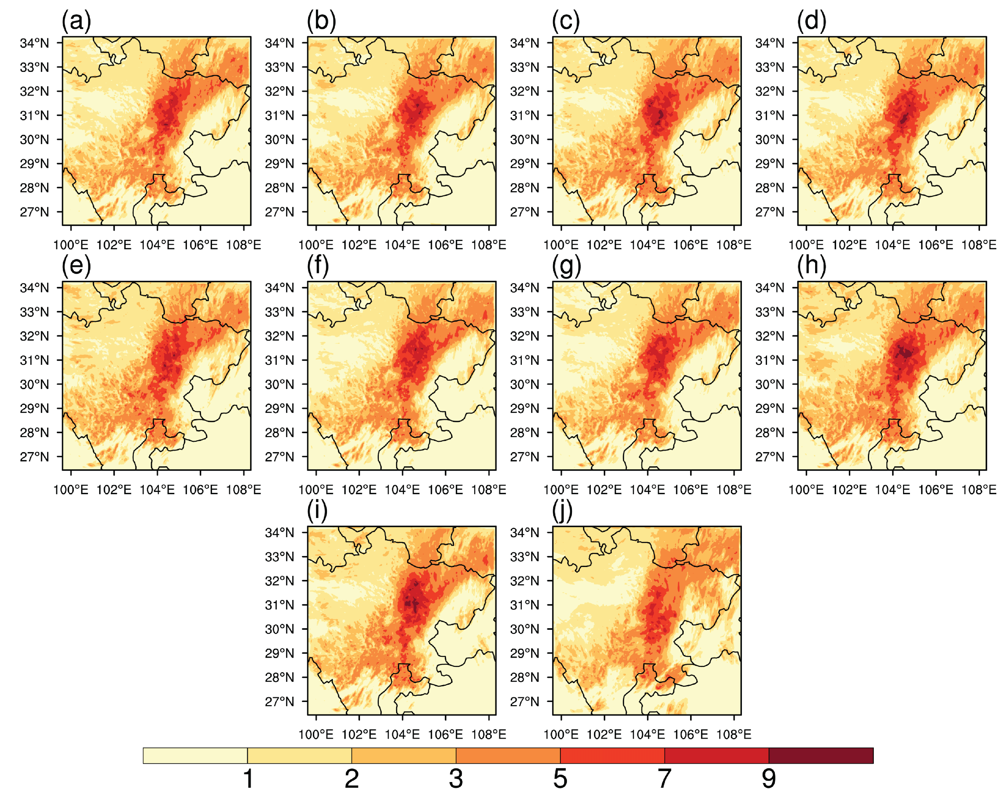
Prior to analyze the uncertainty in the different combinations of physical schemes, verification of the WRF model’s ability of forecasting rainfall over the Sichuan Basin is necessary. To this end, the ensemble mean (48 members) for all cases is calculated, and the results are plotted in Figure 5a–d, respectively. Compared to the corresponding observations (shown in Figure 3a–d), all cases capture the horizontal structure of rainfall well, though the forecasting skill for Case1 is lower than others. However, the center of the predicted heavy precipitation of Case1 is shifting north while a bit south for Case2, Case3, and Case4. We also show the bias of the rainfall forecasts in Figure 5e–h. Note that the significant bias is generally located in the areas of heavy precipitation because of the shift of the center of heavy rainfalls. Except for that, the bias ranges from −15 mm to 15 mm in most areas. These results substantiate that the WRF model ensemble has reasonably good forecasting skills in predicting rainfall events over the Sichuan Basin. However, the performance of individual members still needs to be explored.

4.2.2. Difference between Physical Schemes

In the present study, we mainly evaluate the impact of individual members on the prediction of 24-h cumulative precipitation. Figure A1 and Figure A2 present the results of 48 members for Case1, indicating that the majority of forecasts can capture the rainfall bands well. A closer look at Figure A1 and Figure A2 reveals that M13, M14, M17, M25, M26, M27, and M35 have better performance than other members, while M7–M12, M16, and the members associated with the Thompson MP scheme always greatly overestimate precipitation. Similar phenomena can be found in other three cases (not shown).

Considering that rainfalls may have a diurnal cycle that is sensitive to different physical schemes, except for evaluating the 24-h accumulated precipitation, we also split the 24 h forecasts into two parts, i.e., 12:00–23:00 UTC (nighttime in local time) and 00:00–12:00 UTC (daytime in local time), to calculate the evaluation metrics, respectively.

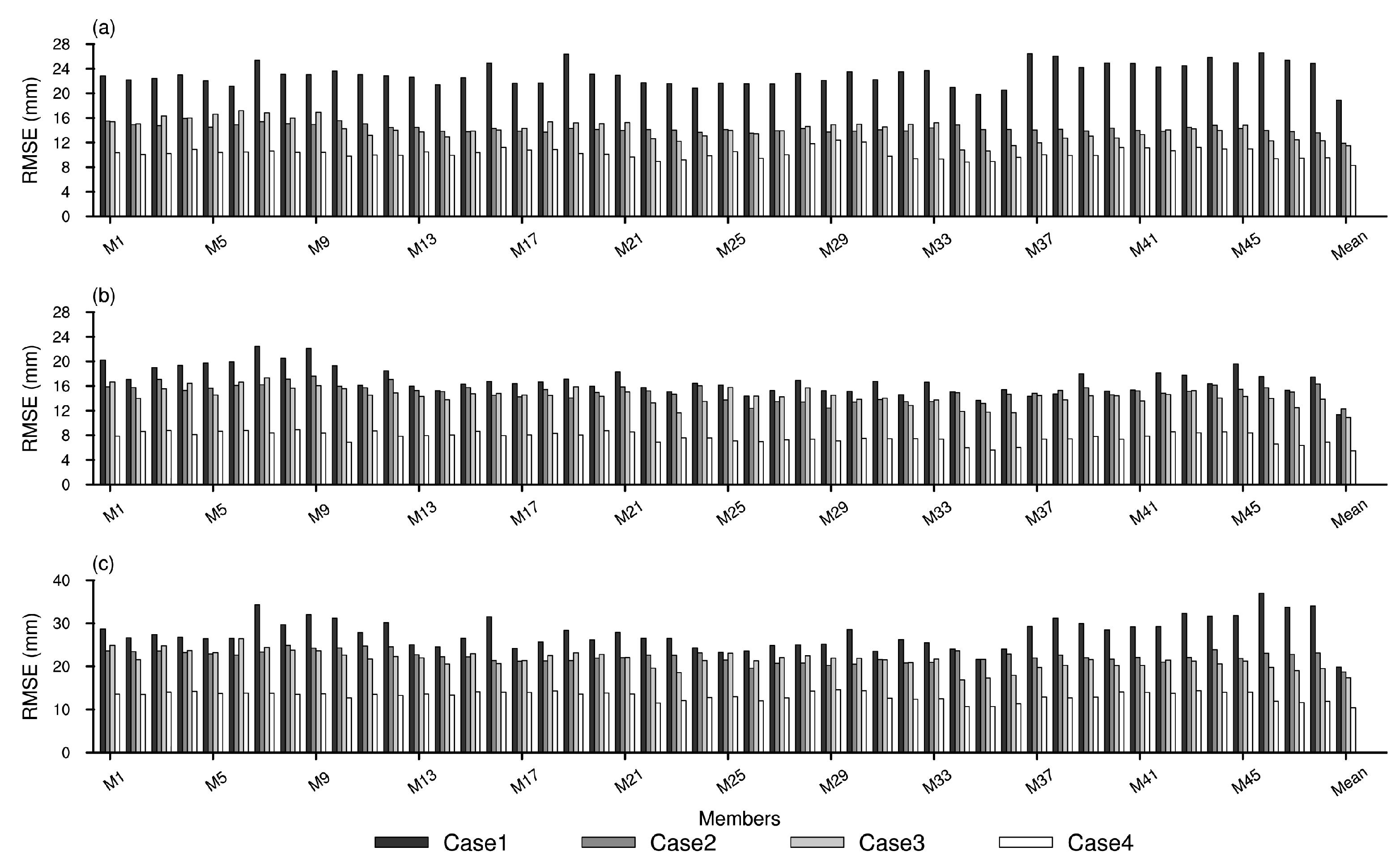
The RMSE between WRF rainfall predictions of different combinations of physical schemes and observations for all cases in three periods is illustrated in Figure 6. In general, it can be observed that Case1 has the largest RMSE while Case4 has the smallest value during all three periods. More importantly, we can find that the variation of RMSE between multi-physics members is significant for four cases. Specifically, for the Case1, the variation of RMSE between multi-physics members ranges in 19.788–26.592 mm, 13.670–22.456 mm, and 21.619–36.990 mm for the period of 12:00–23:00 UTC, 00:00–11:00 UTC and 12:00–11:00 UTC, respectively. Moreover, the STD of RMSE for Case1 during different periods has been calculated and summarized in the second column of

Table 6. The STD (mm) values of RMSE for 48 ensemble members during three periods.

Period	Case1	Case2	Case3	Case4	Mean
12:00–23:00 UTC	1.681	0.556	1.542	0.785	0.745
00:00–11:00 UTC	2.031	1.181	1.266	0.807	1.107
24 h	3.370	1.218	1.904	0.986	1.253

. Those results indicate that the WRF model indeed has a relatively significant difference in the forecasting ability of rainfall when employing different parameterization schemes in the Sichuan Basin. Similar conclusions can be obtained from other cases. Furthermore, we can find that most members associated with WSM6 and Goddard MP schemes (M13–M36) have smaller RMSEs. Note that the mean of ensemble members performs much better than any individuals for all cases.

Figure 7 illustrates the four-case averaged MAEs in the three periods. The results indicate that most experimental runs capture the rainfall intensity and spatial distribution well. However, the oblivious variation among individual members can be observed. Relatively large MAE values occur in members associated with the Lin MP scheme, which indicates that the Lin MP scheme may be not appropriate for the rainfall prediction over the Sichuan Basin.

We then calculate the four-case averaged ETS (Figure 8) to show the performance of each member in five classes of precipitation (shown in Table 2). Consistent with the RMSE, the ETS of ensemble mean shows better skills than most individuals in 12-h and 24-h cumulative precipitation, especially for the light rain, moderate rain, and storm. It can be found that the variation in ETS values of storm and heavy storm is larger than the variation in other intensities of precipitation during all three periods. Besides, for the storm and heavy storm, better forecasting skills are presented when using the WSM6 MP scheme in combination with the ACM2 PBL scheme (M22–M24), the Goddard MP scheme in combination with the YSU PBL scheme (M25–M27), and the Goddard MP scheme in combination with the ACM2 PBL scheme (M34–M36) during three periods, except for heavy storm during 00:00–11:00 UTC. It should be noted that although the members do not display consistent performance in each magnitude of precipitation, the configuration of parameterization schemes is more sensitive to storm and heavy storm.

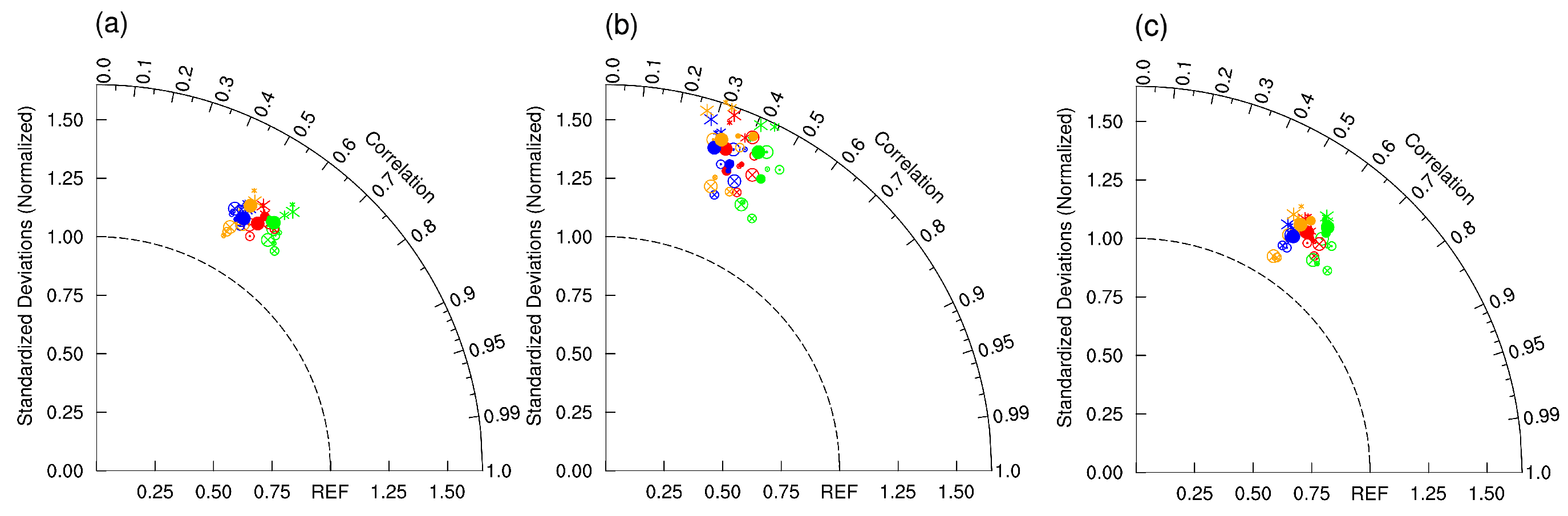
The Taylor diagram displayed in Figure 9 also shows the difference in the performance of the various parametrization schemes. It can be observed that the uncertainty in the rainfall predictions employing multi-physics combinations is large, especially during 00:00–11:00 UTC. From Figure 9c, we can find that the Goddard MP scheme in combination with the ACM2 PBL scheme outperforms others, and the sensitivity of the MP scheme is also strong, with a large spread between the statistics of Lin and Goddard schemes.

4.2.3. Identifying the Well-Performing Physics Scheme Combination

As mentioned above, different combinations of physical schemes perform differently, some of which may have much worse forecasting skills compared to others. Ensemble forecasting is a common way to reduce such uncertainties (as displayed in Figure 6); however, the increasing computational burden may make the operational forecasts impossible. Although the main purpose of this work is not to find the best combinations of multi-physics but to quantify the uncertainty, we also try to identify the most adaptable physics schemes that can be used in the Sichuan Basin, which could be a reference for others’ work. Similar to [8], three normalized metrics, i.e., RMSE, MAE, and reciprocal CC are combined to comprehensively evaluate the prediction ability of WRF model with different parameterizations. We first calculate the three metrics of the 48 WRF runs separately for four cases during different periods and then calculate the mean of those three metrics. Lastly, we obtain the four-case averaged 48 values in three periods, which can be used to calculate the interquartile range (IQR).

Next, we employ a step-wise approach based on IQR to conduct the evaluation. That is, if the value of one scheme for a certain physical scheme is relatively small and at the same time there is less overlap with other options whose values are large, this physical option is deemed as a robust choice that should be retained. When the overlap between different options of a physical scheme is relatively large, there is not necessary to make a choice and they all progress to the next step. After keeping some options of one physical scheme for the first time, we continue to calculate the IQR again by the remaining members. Repeat in turn until the best performing member is selected.

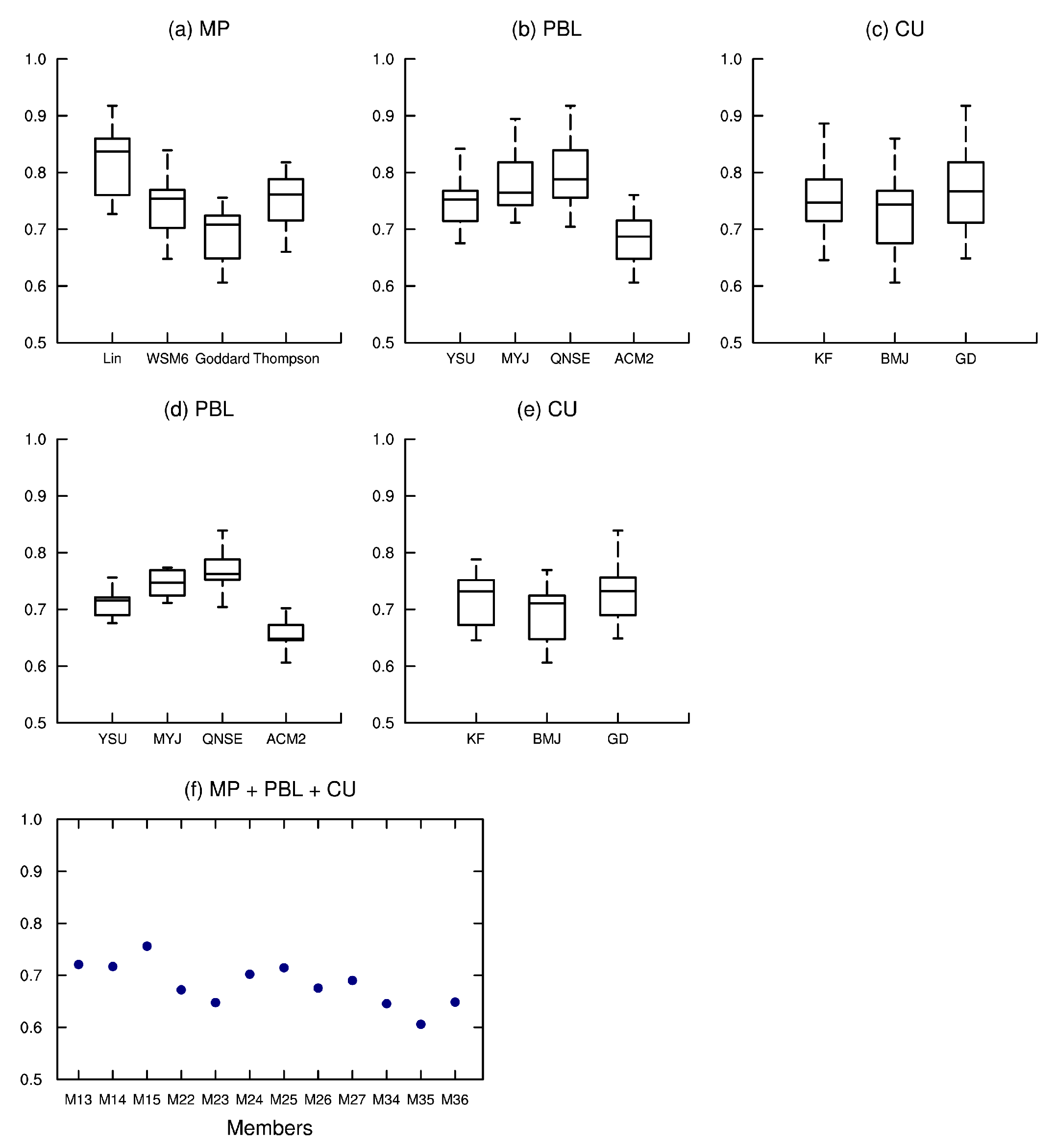
The results for three periods are summarized in Figure 10, Figure 11 and Figure 12 respectively, each row of which represents an evaluation. The size of boxes provides a visual indication of the sensitivity of these schemes. The first row of box plots presents the mean metric for different options of three physical parameterization schemes. From the result of 12-h cumulative precipitation in nighttime (shown in Figure 10), we can find a large overlap of options in MP and CU schemes, which suggests that it is unnecessary to choose them. On the contrary, the YSU and ACM2 PBL schemes have smaller values and less overlap with the other two PBL options; therefore, the members in the second row contain only these two options in the PBL scheme. Although the values of the remaining members vary slightly (Figure 10d), it still can be found that M35 outperforms others. The scenario of 12-h cumulative precipitation in daytime is shown in Figure 11 and it is consistent with the results of 24-h cumulative precipitation (Figure 12). It can be found that Lin and Thompson MP schemes have larger values and less overlap with the other two MP options, and thus both of them are eliminated. Besides, all of the members in the second row contain only the WSM6 and Goddard MP schemes and the MYJ and QNSE PBL schemes are not robust choices ( Figure 11d and Figure 12d). Therefore, the third row of Figure 11 and Figure 12 keeps all the remaining well-simulated members due to the lack of sufficient ensemble members for the next exclusion step. The results indicate that M35 performs best, followed by M34, M36, M23, M22, and M26. There is no significant difference between the nighttime and daytime in choosing the optimal multi-physics ensemble member.

Finally, to guarantee the rationality of the conclusions, we further apply a spatial test to evaluate the simulations from multiple perspectives. Figure 13 depicts the results of SAL metric for the 12 members filtered from the box plots. The S values of all these schemes during three periods are negative, mainly because the simulated maximum precipitation amounts are larger than the corresponding observations. The value of S during three periods for M35 and M36 is closer to 0 compared to others. The A value for three periods ranges from 0.057 to 0.157, 0.122 to 0.312, and 0.101 to 0.192, respectively. During the whole rainfall period, M22, M23 M26, and M34-M36 have better scores than others. The overall change in L value is small. It is worthwhile to mention that the well-performing combinations recognized by the step-wise approach also have a very acceptable skill in the evaluation of the rainfall structure, amplitude, and location.

Based on the above results, it may be concluded that there is an apparent uncertainty in adopting different configurations of physics schemes to predict rainfall over the Sichuan Basin. It is necessary to quantify the uncertainties in those combinations to obtain the optimal rainfall forecasts in the study area. Most metrics show that M35 has the best performance, followed by M34, M36, M23, M22 and M26, in the summer rainfall prediction over the Sichuan Basin.

4.3. Results of Parametric Uncertainty Quantification

Although the uncertainties in the WRF rainfall prediction in terms of the configuration of different physics schemes can be determined to some extent by employing an ensemble run, many uncertainties inside of each scheme are usually neglected, for example, the uncertainty resulting from a lack of knowledge about an empirical parameter whose actual value exhibits no substantial variability. In contrast, the uncertainty in such parameters has a massive impact on the performance and state of an NWP model sometimes. This motivates research into the use of UQ approaches to quantify those uncertainties. The present study employs a non-intrusive UQ approach, i.e., PCE, to propagate the parametric uncertainties to the WRF output of precipitation.

Ten parameters (shown in Table 4), and Case1 and Case2 are chosen to study the parametric uncertainty in the WSM6 MP, YSU PBL, and KF CU schemes which may have a consequential impact on rainfall prediction in the Sichuan Basin.

4.3.1. Impact of the Parametric Uncertainty on 24-h Cumulative Precipitation

The STD of the 24-h cumulative precipitation for the tested parameters over the whole domain are computed by the stochastic collocation method described in Section 3.1, and shown in Figure 14 and Figure 15 for Case1 and Case2, respectively. It is observed that STD has a large variation in the study domain and the prominent STDs distribute mainly in the areas of heavy rain for both cases. The maximum of STD is around 9 mm.

Table 7. Spatial averaged STD values of 24-h cumulative precipitation (mm) in the study domain.

Experiment	P1	P2	P3	P4	P5	P6	P7	P8	P9	P10
Case1	1.704	1.745	1.889	1.772	1.900	1.726	1.663	2.015	1.888	1.813
Case2	1.287	1.348	1.561	1.402	1.553	1.360	1.255	1.670	1.545	1.382
Mean	1.500	1.547	1.725	1.587	1.727	1.543	1.459	1.843	1.717	1.598

summarizes the whole domain averaged STDs for ten uncertain parameters (P1-P10) and a relatively significant difference among ten parameters can be found. The largest value of STD is found for P8 (2.015 mm), reflecting that the uncertainty in the profile shape exponent in the YSU PBL scheme has the most significant impact on the WRF rainfall prediction over the Sichuan Basin. In addition, the impacts of P3 and P5 in the WSM6 MP scheme and P9 in the YSU PBL scheme are also very significant.

We also consider the scenario only in the heavy rainfall area (103° E–106° E, 29° N–33° N) and the results are summarized in

Table 8. Spatial averaged STD values for 24-h cumulative precipitation (mm) in the heavy rain area.

Experiment	P1	P2	P3	P4	P5	P6	P7	P8	P9	P10
Case1	3.552	3.602	3.936	3.807	3.820	3.816	3.656	4.139	4.023	3.527
Case2	1.861	1.883	2.273	2.163	2.219	2.099	1.965	2.472	2.258	2.035
Mean	2.707	2.743	3.105	2.985	3.020	2.958	2.811	3.306	3.141	2.781

. The largest STD of Case1 reaches 4.139 mm for P8. Two-case averaged STD also indicates that P8 is the most significant one, followed by P9, P3 and P5. It should be noted that P3, P5, and P8 are also the sensitive parameters concluded by Ref. [56] which used the MOAT method to study the sensitivity of parameters in summer rainfall over the Greater Beijing Area. This might indicate that most of the uncertain parameters in physics schemes may have similar impacts in different areas.

4.3.2. Impact of the Parametric Uncertainty on Hourly Precipitation

To further investigate the uncertain parameters’ impact on precipitation forecasts over the Sichuan Basin, we choose the small region (103° E–106° E, 29°–33° N) with relatively large 24-h cumulative precipitation for the following study. Figure 16 shows the impact of uncertain parameters on hourly precipitation in two rainfall cases using the IQR boxes, and also shows mean of the predicted hourly precipitation calculated by PCE approach (blue dot) as well as the corresponding observation (black dot).

The boxes are drawn based on hourly precipitation normalized by their mean value. It can be seen that although the mean values of the predicted hourly precipitation for each parameter vary slightly, at most moments there are large discrepancies between them and observation. Furthermore, the variation of boxes shows that the effect of each parameter on hourly precipitation is significant, especially for P3, P5, P8, and P9. It is worth noting that almost every parameter is less sensitive from 12:00 UTC to 23:00 UTC than 0:00 UTC to 11:00 UTC, and the last four hours have the greatest variability in hourly precipitation, indicating that the impact of uncertainty in parameters becomes significant with forecasting lead time.

Therefore, we split the 24 h into two periods, i.e., 12:00 UTC to 23:00 UTC and 0:00 UTC to 11:00 UTC, to show the impact of uncertain parameters on rainfall prediction at different forecasting lead times. The 12-h mean STD of tested parameters during each period is plotted in Figure 17. Consistent with the results in Figure 16, the STD values for all parameters from 0:00 UTC to 11:00 UTC (solid light gray bar) are much larger than that from 12:00 UTC to 23:00 UTC (solid black bar), especially for parameters P1–P3 and P6–P8. The difference between two periods for P9 is minor.

4.3.3. Impact of the Parametric Uncertainty on Other Variables

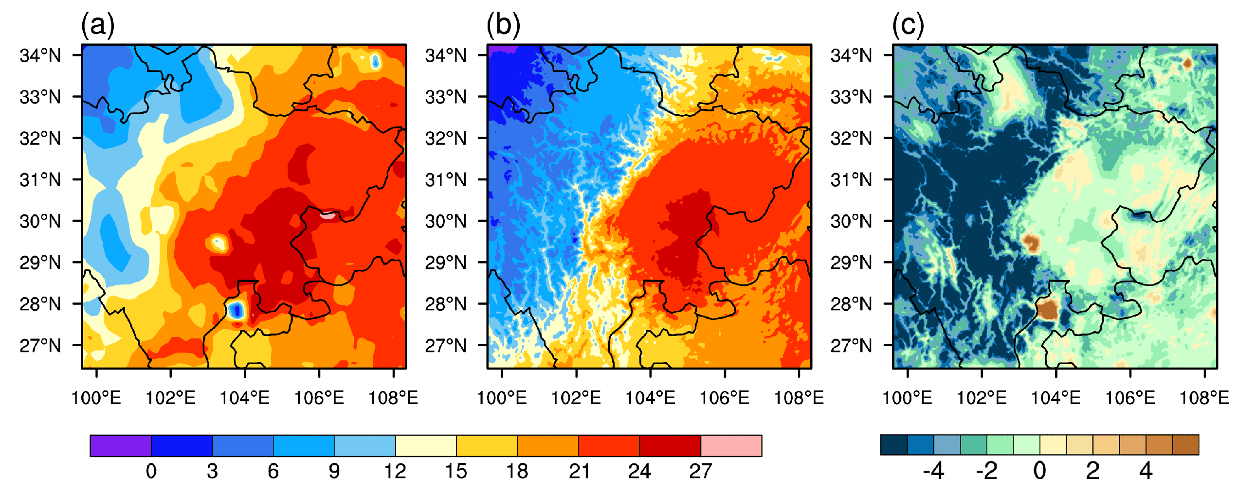
In this section, we examine the impact of uncertain parameters on two additional variables, i.e., 2-m temperature and 2-m dew point temperature. Figure A3–Figure A6 show the validation results of the WRF prediction of these two variables with default values for parameters P1–P10. It is found that the predicted 2-m temperature and dew point temperature fit well with the station observation during different periods in general, although there are relatively large biases on the east of the Tibetan Plateau.

The results of spatial distributions of the STD values for 12-h averaged 2-m temperature are depicted in Figure 18 and Figure 19. It can be observed that the STD of 2-m temperature has a relatively large variation in the study domain, indicating the significant impact caused by the uncertain parameters, among which P3, P5 and P8 influence the forecasts more dominantly than others in both periods. Besides, the STD values for each parameter are significantly larger during daytime than nighttime.

Consistent with the results of 2-m temperature, the STD values of 24-h averaged 2-m dew point temperature (Figure 20) for each uncertain parameter vary obviously in the area of interest. It is also found that the impact on dew point temperature forecasts of the uncertain parameter of P5 and P8 is more significant than other parameters. These results illustrate that the uncertainties in the parameters in the WRF physics schemes not only can affect the forecasting skill of rainfall itself but also have an impact on other rainfall-related variables.

5. Conclusions

This work focused on the challenges presented when forecasting rainfall in regions of complex geographical features, for example, the Sichuan Basin, where the behavior of uncertainties in the parameterization schemes of the WRF model may be more complex than usual. Intending to quantify those uncertainties to some extent, we have conducted a multi-physics ensemble run and employed the PCE approach to examine the difference among multi-combination of physics schemes and the impact of uncertain parameters inside specific schemes, respectively, based on four heavy rainfall processes happened in the Sichuan Basin in summer. We mainly focused on the three kinds of parameterization schemes, i.e., MP, PBL, CU, and verified the results using a couple of metrics. It was observed that most ensemble members have the ability to reproduce the horizontal structure of four rainfall events, however, a significant difference can be found, for example, the variation of the RMSEs between multi-physics ensemble for Case1 during three periods ranges in 19.788–26.592 mm, 13.670–22.456 mm, and 21.619–33.990 mm, respectively. Combining normalized RMSE, MAE and CC, it was found that M22 (WSM6 + ACM2 + KF), M23 (WSM6 + ACM2 + BMJ), M26 (Goddard + YSU + BMJ), M34 (Goddard + ACM2 + KF), M35 (Goddard + ACM2 + BMJ), and M36 (Goddard + ACM2 + GD) have the optimal forecast performance in 12-h and 24-h cumulative precipitation. This result indicated that the Goddard MP scheme together with the ACM2 PBL scheme outperforms other combinations. The possible reason is that the ACM2 scheme can simulate both transport processes generated by large-scale turbulent vortices and capture turbulent mixing processes at small sub-grid scales under convective conditions.

PCE-WRF results indicated that uncertainty in ten empirical parameters has significant impact on the WRF rainfall prediction, especially the scaling factor applied to ice fall velocity (P3), the limited maximum value for the cloud-ice diameter (P5), the profile shape exponent (P8), and the coefficient for Prandtl number (P9). Moreover, it was found that the impact of uncertainty of most empirical parameters becomes more significant with forecasting lead time from the analysis of hourly rainfall prediction. In addition, those parametric uncertainties also influenced the forecasts of 2-m temperature and dew point temperature.

Although we have mainly presented the uncertainty quantification in the region of the Sichuan Basin, we can say without a doubt that this can be applied for other areas of interest. The present study sheds light on the importance of these schemes for the rainfall predictions and other related variables and suggests the next step to improve the physical scheme further. Further work under-way includes repeating this analysis on additional events during different seasons and then developing an operational forecasting system based on the multi-physics ensemble. In addition, developing a framework for improving the uncertain parameters using available observations is also necessary.

References

1. Croitoru, A.E.; Chiotoroiu, B.C.; Todorova, V.I.; Torică, V. Changes in precipitation extremes on the Black Sea Western Coast. Glob. Planet. Change 2013, 102, 10–19. [Google Scholar] [CrossRef]
2. Xiao, C.; Wu, P.; Zhang, L.; Song, L. Robust increase in extreme summer rainfall intensity during the past four decades observed in China. Sci. Rep. 2016, 6, 38506. [Google Scholar] [CrossRef] [PubMed] [Green Version]
3. Francipane, A.; Pumo, D.; Sinagra, M.; La Loggia, G.; Noto, L.V. A paradigm of extreme rainfall pluvial floods in complex urban areas: The flood event of 15 July 2020 in Palermo (Italy). Nat. Hazards Earth Syst. Sci. Discuss. 2021, 21, 2563–2580. [Google Scholar] [CrossRef]
4. Buehner, M.; Morneau, J.; Charette, C. Four-dimensional ensemble-variational data assimilation for global deterministic weather prediction. Nonlinear Process. Geophys. 2013, 20, 669–682. [Google Scholar] [CrossRef] [Green Version]
5. Xu, D.; Min, J.; Shen, F.; Ban, J.; Chen, P. Assimilation of MWHS radiance data from the FY-3B satellite with the WRF Hybrid-3DVAR system for the forecasting of binary typhoons. J. Adv. Model. Earth Syst. 2016, 8, 1014–1028. [Google Scholar] [CrossRef] [Green Version]
6. Che, Y.; Chen, C.; Xiao, F.; Li, X.; Shen, X. A Two-Stage Fourth-Order Multimoment Global Shallow-Water Model on the Cubed Sphere. Mon. Weather. Rev. 2020, 148, 4267–4279. [Google Scholar] [CrossRef]
7. Ricchi, A.; Miglietta, M.M.; Bonaldo, D.; Cioni, G.; Rizza, U.; Carniel, S. Multi-physics ensemble versus atmosphere–ocean coupled model simulations for a tropical-like cyclone in the Mediterranean Sea. Atmosphere 2019, 10, 202. [Google Scholar] [CrossRef] [Green Version]
8. Evans, J.P.; Ekström, M.; Ji, F. Evaluating the performance of a WRF physics ensemble over South-East Australia. Clim. Dyn. 2012, 39, 1241–1258. [Google Scholar] [CrossRef]
9. Yang, M.x.; Jiang, Y.z.; Lu, X.; Zhao, H.l.; Ye, Y.t.; Tian, Y. A weather research and forecasting model evaluation for simulating heavy precipitation over the downstream area of the Yalong River Basin. J. Zhejiang Univ.-Sci. A 2015, 16, 18–37. [Google Scholar] [CrossRef] [Green Version]
10. Liu, Y.; Chen, Y.; Chen, O.; Wang, J.; Zhuo, L.; Rico-Ramirez, M.A.; Han, D. To develop a progressive multimetric configuration optimisation method for WRF simulations of extreme rainfall events over Egypt. J. Hydrol. 2021, 598, 126237. [Google Scholar] [CrossRef]
11. Yang, Q.; Yu, Z.; Wei, J.; Yang, C.; Gu, H.; Xiao, M.; Shang, S.; Dong, N.; Gao, L.; Arnault, J.; et al. Performance of the WRF model in simulating intense precipitation events over the Hanjiang River Basin, China–A multi-physics ensemble approach. Atmos. Res. 2021, 248, 105206. [Google Scholar] [CrossRef]
12. Jiang, X.; Li, Y.; Zhao, X.; Koike, T. Characteristics of the summertime boundary layer and atmospheric vertical structure over the Sichuan basin. J. Meteorol. Soc. Jpn. Ser. II 2012, 90, 33–54. [Google Scholar] [CrossRef] [Green Version]
13. Gao, D.; Li, Y.; Jiang, X.; Li, J.; Wu, Y. Influence of planetary boundary layer parameterization schemes on prediction of rainfall with different magnitudes in the sichuan basin using the WRF model. Chin. J. Atmos. Sci. 2016, 40, 371–389. (In Chinese) [Google Scholar]
14. Zhu, K.Y.; Zhang, J.L.E. Experimental study on different cumulus parameterization schemes in WRF model over Sichuan. J. Chengdu Univ. Inf. Technol. 2014, 29, 71–81. (in Chinese). [Google Scholar]
15. Qiu C, C.J. A new approach to improve the numerical weather prediction. Sci. China Ser. B 1988, 9, 1132–1142. [Google Scholar]
16. Hong, S.Y.; Dudhia, J.; Chen, S.H. A revised approach to ice microphysical processes for the bulk parameterization of clouds and precipitation. Mon. Weather. Rev. 2004, 132, 103–120. [Google Scholar] [CrossRef]
17. Nielsen-Gammon, J.W.; Hu, X.M.; Zhang, F.; Pleim, J.E. Evaluation of planetary boundary layer scheme sensitivities for the purpose of parameter estimation. Mon. Weather. Rev. 2010, 138, 3400–3417. [Google Scholar] [CrossRef] [Green Version]
18. Di, Z.; Duan, Q.; Gong, W.; Ye, A.; Miao, C. Parametric sensitivity analysis of precipitation and temperature based on multi-uncertainty quantification methods in the Weather Research and Forecasting model. Sci. China Earth Sci. 2017, 60, 876–898. [Google Scholar] [CrossRef]
19. Hastings, W.K. Monte Carlo sampling methods using Markov chains and their applications. Biometrika 1970, 57, 97–109. [Google Scholar] [CrossRef]
20. Halton, J.H. Algorithm 247: Radical-inverse quasi-random point sequence. Commun. ACM 1964, 7, 701–702. [Google Scholar] [CrossRef]
21. Caflisch, R.E. Monte carlo and quasi-monte carlo methods. Acta Numer. 1998, 7, 1–49. [Google Scholar] [CrossRef] [Green Version]
22. Box, G.E.; Hunter, J.S.; Hunter, W.G. Statistics for Experimenters: Design, Innovation, and Discovery; Wiley-Interscience: New York, NY, USA, 2005; Volume 2. [Google Scholar]
23. McKay, M.D.; Beckman, R.J.; Conover, W.J. A comparison of three methods for selecting values of input variables in the analysis of output from a computer code. Technometrics 2000, 42, 55–61. [Google Scholar] [CrossRef]
24. Qian, Y.; Yan, H.; Hou, Z.; Johannesson, G.; Klein, S.; Lucas, D.; Neale, R.; Rasch, P.; Swiler, L.; Tannahill, J.; et al. Parametric sensitivity analysis of precipitation at global and local scales in the Community Atmosphere Model CAM5. J. Adv. Model. Earth Syst. 2015, 7, 382–411. [Google Scholar] [CrossRef] [Green Version]
25. Morris, T.; Wood, S. Testing the survey method: Continuity and change in British industrial relations. Work. Employ. Soc. 1991, 5, 259–282. [Google Scholar] [CrossRef]
26. Li, J.; Duan, Q.; Gong, W.; Ye, A.; Dai, Y.; Miao, C.; Di, Z.; Tong, C.; Sun, Y. Assessing parameter importance of the Common Land Model based on qualitative and quantitative sensitivity analysis. Hydrol. Earth Syst. Sci. 2013, 17, 3279–3293. [Google Scholar] [CrossRef] [Green Version]
27. Najm, H.N. Uncertainty quantification and polynomial chaos techniques in computational fluid dynamics. Annu. Rev. Fluid Mech. 2009, 41, 35–52. [Google Scholar] [CrossRef]
28. Xiu, D.; Karniadakis, G.E. The Wiener–Askey polynomial chaos for stochastic differential equations. SIAM J. Sci. Comput. 2002, 24, 619–644. [Google Scholar] [CrossRef]
29. Xiu, D. Numerical Methods for Stochastic Computations; Princeton University Press: Princeton, NJ, USA, 2010. [Google Scholar]
30. Palar, P.S.; Zuhal, L.R.; Shimoyama, K.; Tsuchiya, T. Global sensitivity analysis via multi-fidelity polynomial chaos expansion. Reliab. Eng. Syst. Saf. 2018, 170, 175–190. [Google Scholar] [CrossRef] [Green Version]
31. Jin, J.; Che, Y.; Zheng, J.; Xiao, F. Uncertainty Quantification of a Coupled Model for Wind Prediction at a Wind Farm in Japan. Energies 2019, 12, 1505. [Google Scholar] [CrossRef] [Green Version]
32. Sepahvand, K.; Marburg, S.; Hardtke, H.J. Uncertainty quantification in stochastic systems using polynomial chaos expansion. Int. J. Appl. Mech. 2010, 2, 305–353. [Google Scholar] [CrossRef]
33. Meng, X.; Cheng, J. Evaluating eight global reanalysis products for atmospheric correction of thermal infrared sensor—Application to Landsat 8 TIRS10 Data. Remote Sens. 2018, 10, 474. [Google Scholar] [CrossRef] [Green Version]
34. Hua, W.; Zhou, L.; Nicholson, S.E.; Chen, H.; Qin, M. Assessing reanalysis data for understanding rainfall climatology and variability over Central Equatorial Africa. Clim. Dyn. 2019, 53, 651–669. [Google Scholar] [CrossRef] [Green Version]
35. Shikhovtsev, A.Y.; Kovadlo, P.; Kiselev, A. Astroclimatic statistics at the Sayan solar observatory. Sol.-Terr. Phys. 2020, 6, 102–107. [Google Scholar]
36. Hach, Y.; Jabiri, A.; Ziad, A.; Bounhir, A.; Sabil, M.; Abahamid, A.; Benkhaldoun, Z. Meteorological profiles and optical turbulence in the free atmosphere with NCEP/NCAR data at Oukaïmeden–I. Meteorological parameters analysis and tropospheric wind regimes. Mon. Not. R. Astron. Soc. 2012, 420, 637–650. [Google Scholar] [CrossRef] [Green Version]
37. Warner, T.T.; Peterson, R.A.; Treadon, R.E. A Tutorial on Lateral Boundary Conditions as a Basic and Potentially Serious Limitation to Regional Numerical Weather Prediction. Bull. Am. Meteorol. Soc. 1997, 78, 2599–2617. [Google Scholar] [CrossRef] [Green Version]
38. Warner, T.T. Quality Assurance in Atmospheric Modeling. Bull. Am. Meteorol. Soc. 2011, 92, 1601–1610. [Google Scholar] [CrossRef] [Green Version]
39. Wang, W.; Bruyère, C.; Duda, M.; Dudhia, J.; Gill, D.; Kavulich, M.; Keene, K.; Chen, M.; Lin, H.C.; Michalakes, J.; et al. ARW Users Guide V3.9-3. 2017. Available online: https://www2.mmm.ucar.edu/wrf/users/docs/user_guide_V3/contents.html (accessed on 17 April 2017).
40. Dudhia, J. Numerical study of convection observed during the winter monsoon experiment using a mesoscale two-dimensional model. J. Atmos. Sci. 1989, 46, 3077–3107. [Google Scholar] [CrossRef]
41. Mlawer, E.J.; Taubman, S.J.; Brown, P.D.; Iacono, M.J.; Clough, S.A. Radiative transfer for inhomogeneous atmospheres: RRTM, a validated correlated-k model for the longwave. J. Geophys. Res. Atmos. 1997, 102, 16663–16682. [Google Scholar] [CrossRef] [Green Version]
42. Tewari, M.; Chen, F.; Wang, W.; Dudhia, J.; LeMone, M.; Mitchell, K.; Ek, M.; Gayno, G.; Wegiel, J.; Cuenca, R.; et al. Implementation and verification of the unified NOAH land surface model in the WRF model. In Proceedings of the 20th Conference on Weather Analysis and Forecasting/16th Conference on Numerical Weather Prediction, Seattle, WA, USA, 14 January 2004; Volume 1115. [Google Scholar]
43. Lin, Y.L.; Farley, R.D.; Orville, H.D. Bulk parameterization of the snow field in a cloud model. J. Appl. Meteorol. Climatol. 1983, 22, 1065–1092. [Google Scholar] [CrossRef] [Green Version]
44. Hong, S.Y.; Lim, J.O.J. The WRF single-moment 6-class microphysics scheme (WSM6). Asia-Pac. J. Atmos. Sci. 2006, 42, 129–151. [Google Scholar]
45. Tao, W.K.; Simpson, J.; McCumber, M. An ice-water saturation adjustment. Mon. Weather. Rev. 1989, 117, 231–235. [Google Scholar] [CrossRef] [Green Version]
46. Thompson, G.; Field, P.R.; Rasmussen, R.M.; Hall, W.D. Explicit forecasts of winter precipitation using an improved bulk microphysics scheme. Part II: Implementation of a new snow parameterization. Mon. Weather. Rev. 2008, 136, 5095–5115. [Google Scholar] [CrossRef]
47. Hong, S.Y.; Noh, Y.; Dudhia, J. A new vertical diffusion package with an explicit treatment of entrainment processes. Mon. Weather. Rev. 2006, 134, 2318–2341. [Google Scholar] [CrossRef] [Green Version]
48. Janjić, Z.I. The step-mountain eta coordinate model: Further developments of the convection, viscous sublayer, and turbulence closure schemes. Mon. Weather. Rev. 1994, 122, 927–945. [Google Scholar] [CrossRef] [Green Version]
49. Sukoriansky, S.; Galperin, B.; Perov, V. A quasi-normal scale elimination model of turbulence and its application to stably stratified flows. Nonlinear Process. Geophys. 2006, 13, 9–22. [Google Scholar] [CrossRef]
50. Pleim, J.E. A combined local and nonlocal closure model for the atmospheric boundary layer. Part I: Model description and testing. J. Appl. Meteorol. Climatol. 2007, 46, 1383–1395. [Google Scholar] [CrossRef]
51. Kain, J.S. The Kain–Fritsch convective parameterization: An update. J. Appl. Meteorol. 2004, 43, 170–181. [Google Scholar] [CrossRef] [Green Version]
52. Grell, G.A.; Dévényi, D. A generalized approach to parameterizing convection combining ensemble and data assimilation techniques. Geophys. Res. Lett. 2002, 29, 38–1–38–4. [Google Scholar] [CrossRef] [Green Version]
53. Skamarock, W.C.; Klemp, J.B.; Dudhia, J.; Gill, D.O.; Barker, D.M.; Wang, W.; Powers, J.G. A description of the Advanced Research WRF version 3. In NCAR Technical Note-475+ STR; University Corporation for Atmospheric Research: Boulder, CO, USA, 2008. [Google Scholar]
54. Wernli, H.; Paulat, M.; Hagen, M.; Frei, C. SAL—A novel quality measure for the verification of quantitative precipitation forecasts. Mon. Weather. Rev. 2008, 136, 4470–4487. [Google Scholar] [CrossRef] [Green Version]
55. Xiu, D. Efficient collocational approach for parametric uncertainty analysis. Commun. Comput. Phys. 2007, 2, 293–309. [Google Scholar]
56. Di, Z.; Duan, Q.; Gong, W.; Wang, C.; Gan, Y.; Quan, J.; Li, J.; Miao, C.; Ye, A.; Tong, C. Assessing WRF model parameter sensitivity: A case study with 5 day summer precipitation forecasting in the Greater Beijing Area. Geophys. Res. Lett. 2015, 42, 579–587. [Google Scholar] [CrossRef]
57. Chen, X.A.; Chen, Y.L. Development of low-level jets during TAMEX. Mon. Weather. Rev. 1995, 123, 1695–1719. [Google Scholar] [CrossRef] [Green Version]
58. Chen, Y.L.; Li, J. Large-scale conditions favorable for the development of heavy rainfall during TAMEX IOP 3. Mon. Weather. Rev. 1995, 123, 2978–3002. [Google Scholar] [CrossRef] [Green Version]
59. Chen, Y.L.; Tu, C.C.; Hsiao, F.; Chen, C.S.; Lin, P.L.; Lin, P.H. An Overview of Low-Level Jets (LLJs) and Their Roles in Heavy Rainfall over the Taiwan Area during the Early Summer Rainy Season. Meteorology 2022, 1, 64–112. [Google Scholar] [CrossRef]
Figure 1. Map showing the parent and a nested domain for the WRF model. Shaded stands for the elevation (m).
Atmosphere 13 00838 g001
Figure 2. The location (black dots) of Chinese ground-based and encrypted stations over the Sichuan region.
Atmosphere 13 00838 g002
Figure 3. (ad) show the observation of 24-h accumulated precipitation (mm) for Case1 to Case4 respectively.
Atmosphere 13 00838 g003
Figure 4. The geopotential height (black contours in dagpm), wind vectors (black arrows, ms−1) and water vapour flux (shaded in g/(cm *hPa*s)) for four cases. The blue line represents the Sichuan provincial boundary. The red dashed lines represent the troughs while solid lines are shear lines. The Western Pacific Subtropical High locations and the center of the Tropical Cyclones are also marked.
Atmosphere 13 00838 g004
Figure 5. (ad) show the ensemble mean of predicted 24-h accumulated precipitation (mm) for Case1 to Case4 respectively. (eh) are the bias (mm) between WRF ensemble mean and observation.
Atmosphere 13 00838 g005
Figure 6. The RMSE (mm) for each ensemble member in Case1 (solid black bar), Case2 (solid dark grey bar), Case3 (solid light grey bar), and Case4 (solid white bar) during 12:00–23:00 UTC (a), 00:00–11:00 UTC (b) and 24 h (c). The result of ensemble mean is also shown.
Atmosphere 13 00838 g006
Figure 7. The four-case averaged MAE (mm) for each ensemble member during 12:00–23:00 UTC (a), 00:00–11:00 UTC (b), and 24 h (c).
Atmosphere 13 00838 g007
Figure 8. The average ETS of light rain (the first row), moderate rain (the second row), heavy rain (the third row), storm (the fourth row), and heavy storm (the fifth row) for each ensemble member in four rainfall cases during 12:00–23:00 UTC (the first column), 00:00–11:00 UTC (the second column), and 24 h (the third column), respectively. “Mean” denotes the ensemble mean.
Atmosphere 13 00838 g008
Figure 9. Taylor diagrams show the four-case averaged normalized standard derivation and correlation for 48 ensemble members during 12:00–23:00 UTC (a), 00:00–11:00 UTC (b) and 24 h (c). Shapes represent the MP schemes: Lin (*), WSM6 (⊙), Goddard (⊗), Thompson (•); colors represent the PBL schemes: YSU (red), MYJ (blue), QNSE (orange), ACM2 (green); sizes represent the CU schemes: KF (small), BMJ (moderate), GD (big).
Atmosphere 13 00838 g009
Figure 10. Box plots of the average metric split by physical parameterization of WRF model during 12:00–23:00 UTC. The second row retains only those members with YSU and ACM2 PBL schemes.
Atmosphere 13 00838 g010
Figure 11. Same as Figure Figure 10, but for the period of 00:00 UTC to 11:00 UTC. The second row retains only those members with WSM6 and Goddard MP schemes, and the third row additionally excludes those members containing MYJ and QNSE PBL schemes.
Atmosphere 13 00838 g011
Figure 12. Same as Figure Figure 10, but for all 24 h. The second row retains only those members with WSM6 and Goddard MP schemes, and the third row additionally excludes those members containing MYJ and QNSE PBL schemes.
Atmosphere 13 00838 g012
Figure 13. The four-case averaged Structure (the first row), Amplitude (the second row) and Location (the third row) metrics of 12 combination members consistent with Figure 10d (the first column), Figure 11g (the second column), and Figure 12g (the third column), respectively.
Atmosphere 13 00838 g013
Figure 14. Spatial distribution of STD values for 24-h cumulative precipitation (mm) of Case1. Panels from (aj) stand for P1 to P10, respectively.
Atmosphere 13 00838 g014
Figure 15. Similar to Figure 14, but for Case2. Panels from (aj) show the results of parameter P1 to P10, respectively.
Atmosphere 13 00838 g015
Figure 16. The IQR boxes of hourly precipitation normalized by their mean values (left axis) for each uncertainty parameter at 24 instants from 12:00 UTC to 11:00 UTC. The blue dots and black dots represent the mean of the simulated hourly precipitation and corresponding observation (right axis), respectively. Panels from (aj) stand for P1 to P10, respectively.
Atmosphere 13 00838 g016
Figure 17. The comparison of the mean STD of hourly precipitation during different periods.
Atmosphere 13 00838 g017
Figure 18. Spatial distribution of STD values for 12-h averaged 2-m temperature (K) during 12:00–23:00 UTC. Panels from (aj) stand for P1 to P10, respectively.
Atmosphere 13 00838 g018
Figure 19. Similar to Figure 18, but for the period of 00:00 UTC to 11:00 UTC.
Atmosphere 13 00838 g019
Figure 20. Spatial distribution of STD values for 24-h averaged 2-m dew point temperature (°C). Panels from (aj) stand for P1 to P10, respectively.
Atmosphere 13 00838 g020