Weather Radar Echo Extrapolation Method Based on Deep Learning

Abstract

In order to forecast some high intensity and rapidly changing phenomena, such as thunderstorms, heavy rain, and hail within 2 h, and reduce the influence brought by destructive weathers, this paper proposes a weather radar echo extrapolation method based on deep learning. The proposed method includes the design and combination of the data preprocessing, convolutional long short-term memory (Conv-LSTM) neuron and encoder–decoder model. We collect eleven thousand weather radar echo data in high spatiotemporal resolution, these data are then preprocessed before they enter the neural network for training to improve the data’s quality and make the training better. Next, the neuron integrates the structure and the advantages of convolutional neural network (CNN) and long short-term memory (LSTM), called Conv-LSTM, is applied to solve the problem that the full-connection LSTM (FC-LSTM) cannot extract the spatial information of input data. This operation replaced the full-connection structure in the input-to-state and state-to-state parts so that the Conv-LSTM can extract the information from other dimensions. Meanwhile, the encoder–decoder model is adopted due to the size difference of the input and output data to combine with the Conv-LSTM neuron. In the neural network training, mean square error (MSE) loss function weighted according to the rate of rainfall is added. Finally, the matrix “point-to-point” test method, including the probability of detection (POD), critical success index (CSI), false alarm ratio (FAR) and spatial test method contiguous rain areas (CRA), is used to examine the radar echo extrapolation’s results. Under the threshold of 30 dBZ, at the time of 1 h, we achieved 0.60 (POD), 0.42 (CSI) and 0.51 (FAR), compared with 0.42, 0.28 and 0.58 for the CTREC algorithm, and 0.30, 0.24 and 0.71 for the TITAN algorithm. Meanwhile, at the time of 1 h, we achieved 1.35 (total MSE ) compared with 3.26 for the CTREC algorithm and 3.05 for the TITAN algorithm. The results demonstrate that the radar echo extrapolation method based on deep learning is obviously more accurate and stable than traditional radar echo extrapolation methods in near weather forecasting.

1. Introduction

The role of the strong convective weather forecast in today’s society is self-evident because the evolution rule is extremely complex, and for agriculture, social activities will have a big impact, easily causing disaster and life and property loss. Therefore, for the inherent laws, the characteristics of the future trends of this kind of weather have been the focus of the all-weather forecast department. The forecast of this kind of weather is called near weather forecasting technology [1]. The near weather forecasting technology is mainly divided into three technologies: extrapolation techniques (which combine identification, tracking and extrapolation), numerical weather prediction technology and expert system model forecasting technology combined with multiple observation data and analysis methods [2,3]. Numerical weather prediction technology contains complex physical equation calculation and it is difficult to satisfy the requirements of accuracy and real-time in precipitation prediction [4]. Expert system model forecasting technology needs hardware support and a personnel assistant, and it should integrate a variety of medium- and small-scale observation data and different weather prediction technologies as well [5,6].

The extrapolation forecasting technology, which has a better performance in the near weather forecast and has been developed fairly maturely, can bring good reference and early warning within 0–2 h. The relatively mainstream algorithms in extrapolation forecasting technology include cross-correlation, monomer centroid and optical flow methods [7]. The first two algorithms have been widely used in many local meteorological forecasting departments [8]. In this paper, we use a cross-correlation method (coordinate tracking radar echoes by correlation (CTREC)) and a monomer centroid method (thunderstorm identification, tracking, analysis and nowcasting (TITAN)) to compare with the weather radar echo extrapolation method based on deep learning.

The cross-correlation method has a good prediction effect on the stratiform cloud weather system and layered and convective mixed weather system with slow change and stable trends. However, the prediction accuracy is low for a severe convective weather system with rapid direction change and complex movement trends [9,10,11,12]. The centroid method [13,14] can effectively track convective cells with high intensity. However, it is not easy to identify echoes with small intensity and complex structures, and storm cells [14,15,16] should not develop too violently; otherwise, tracking can easily fail. The two extrapolation methods still have some defects. Therefore, the extrapolation prediction technology based on a deep learning algorithm has been developed.

Deep learning is built based on the machine learning algorithms and theories. It is also developed to satisfy the requirements of artificial intelligence [17]. The deep learning model is usually an end-to-end model, under this circumstance, we only need to feed the data and then obtain the output results. So, deep learning does not require very expert professional knowledge for users. In recent years, deep learning has made major breakthroughs in technologies and theories [18], showing excellent abilities in many fields. Through the formulation of an optimization algorithm, the construction of a neural network model and learning or training a large amount of data, the neural network using deep learning algorithms can effectively “learn” the internal correlation of the radar data features in high spatiotemporal resolution sequences, capturing the evolution law and motion state of the radar echo quickly. At present, the near weather forecasting based on deep learning is mainly realized by radar echo extrapolation [19,20,21,22,23]. Compared with CTREC or TITAN, the deep learning model can overcome their disadvantages, tracking and forecasting severe convective weather more stably and more accurately. Additionally, with the development of deep learning, the weather radar extrapolation method based on deep learning has greater potential.

Meanwhile, there are several high-resolution data in the meteorological field, such as radar-based data obtained by traditional single-polarization and more advanced dual-polarization Doppler radar, as well as real-time observation data from ground observation stations and satellite data [24,25]. The amount of data is very large that it is appropriate to combine the data with deep learning. If we can build a deep learning neural network model with a computing-intensive server, to train and learn these data, save an end-to-end model and directly deploy it in the weather forecast operational system, the real-time prediction ability of minutes or seconds is expected to be realized. Then, it will be essential in developing weather forecast services.

The main contributions of this paper are as follows:

(1)

Read quantities of weather radar data from radar-based data. The benefits of massive data for deep learning are shown in this paper.

(2)

Choose effective data quality control methods to filter the clutter. Use the best in three interpolation methods.

(3)

Find the appropriate parameters suitable for the neural network.

(4)

Select a reasonable loss function and set up a weight matrix to assist the training of neural network.

(5)

Make multiple tables according to the experiment results and evaluation criteria to approve the accuracy of the deep learning system.

This paper includes six sections. The first section is the introduction, to introduce the background of near weather forecasting technology, illustrate the practicability and superiorities of deep learning system. The second section gives the data preprocessing methods for producing data input and improving training quality. The third section introduces the core principles and algorithms of deep learning methods. The fourth section explains the evaluation criteria of extrapolation results, so that we can verify the results from different aspects. The fifth section presents all quantitative result analyses and figure displays of the traditional extrapolation algorithms and deep learning algorithm. The final section shows the conclusions and prospects of this paper.

2. Data Preprocessing

Not only does the new generation of weather radar detect the meteorological targets, but it detects the non-meteorological targets. The quality of weather radar echo data has a direct impact on the extrapolation experiments. The main factors affecting the quality of data are the ground clutter and noise clutter. These two kinds of clutter will affect the performance of radar echo measuring the precipitation, and the integrity of echo display. They will also affect the feature extraction, target judgment and result calculation in the extrapolation experiment. So, we used the weather radar echo data quality control algorithms to filter this clutter. Then, the data after quality control will be interpolated. The data in polar coordinates will be interpolated into the plane grid. Finally, the interpolated data are normalized and sent to the extrapolation method as input. The flowchart of the data preprocessing is shown in Figure 1:

2.1. Data Quality Control

2.1.1. Noise Clutter

For the noise clutter, the method of filtering out the isolated points and making up the missing detection points is adopted.

Filtering isolated points requires traversing every radar echo database, and if it is valid, a rectangular window $N\ast N$ is created on the data. Then, the total number of valid data $M$ and the proportion of valid data $S$ of all data in the window are obtained. Finally, a threshold of $M_0$ (typically set to 0.7, it is verified that the threshold between 0.5 and 0.7 is effective to filter isolated points) is set to determine the isolated point. Meanwhile, if $S$ is less than $M_0$, it will be judged as an isolated point and set as invalid data. The specific equation is as follows:

$$S=M/N^2$$

(1)

Filling in a missing point is also known as the alopecia areata problem. Similar to the method of filtering the isolated points, this method requires traversing the radar echo database and creating a rectangular window $M\ast M$ on the traversal point (the size of the window in this paper is $M=5$; this value is an appropriate value concluded throughout experiments), then counting the number of valid data in the $M\ast M$ window and set a threshold value (the default value is 12; the threshold value can be around 12, which goes up to the number of points that you want to fill in). If the number of valid data exceeds this threshold, the target grid point is replaced with

$$V=\frac{1}{M^2}{\displaystyle \sum _{i=1}^{M^2}{V}_i}$$

(2)

Here, $V_i$ is the value of the ith data in the window. The specific schematic diagram is shown in Figure 2.

2.1.2. Ground Clutter

In this paper, the recognition of ground object clutter is mainly judged by three factors: reflectivity factor mean radial texture $\left(TDBZ\right)$, reflectivity factor vertical gradient $\left(VGZ\right)$ and absolute radial velocity $\left(V_{abs}\right)$ [26,27]. Ground clutter significantly differs from the meteorological echo from these three aspects. These three values are calculated as follows:

$$\begin{array}{l}TDBZ={\left({\displaystyle \sum _{j=1}^{N_{radials}}{\displaystyle \sum _{i=2}^{N_{gates}}{\left(X_{i,j,k}-X_{i-1,j,k}\right)}^2/N}}\right)}^{\frac{1}{2}}\\ VGZ=\frac{Z_{low}-Z_{up}}{H_{up}-H_{low}}\\ V_{abs}=\left|V\right|\end{array}$$

(3)

Here, $i$ and $j$ represent the range bin number and radial number of the reflectivity factor, respectively; $N_{gates}$ and $N_{radials}$ represent the number of range bin number and radial number in the sector region centered on the reflectivity coordinates $i$ and $j$, respectively. In this paper, the size of $N_{gates}$ and $N_{radials}$ is set to 5 (this value is an appropriate value concluded throughout experiments). It is more effective to use $TDBZ$ to judge ground clutter and precipitation echo in places far away from the radar center (range > 150 km), and the $TDBZ$ of ground clutter is relatively larger.

The vertical gradient of reflectivity $\left(VGZ\right)$ reflects the variation characteristics of echo on the vertical gradient. It is an essential feature to identify precipitation echo and ground clutter. Ground clutter usually appears at low elevation; however, it disappears as the elevation increases. Therefore, the $\left(VGZ\right)$ ground clutter is generally large. In the calculation equation of $\left(VGZ\right)$, $Z_{low}$ represents the reflectivity factor value at the low elevation, $Z_{up}$ represents the reflectivity factor value at the high elevation with the same azimuth and range bin number, $H_{up}$ and $H_{low}$ represent the corresponding height, where the reference height $H_{up}$ is 3–4.5 km and $H_{low}$ is the corresponding height at the low elevation.

Additionally, $V_{abs}$ represents the radial velocity corresponding to the azimuth and range bin number. Because the resolution of radial velocity and reflectivity factor is different, the range bin of radial velocity is four times that of the reflectivity factor. Therefore, four consecutive grid points in the radial direction correspond to a range bin of reflectivity factors.

2.2. Data Interpolation

Data interpolation transforms the data points in the plane grid region of the Cartesian coordinate system (hereinafter referred to as Cartesian coordinate system) into the polar coordinate system centered on the radar station. Then, the polar coordinates of the grid point $P\left(x,y,z\right)$ in the Cartesian coordinate system are transformed as follows:

$$\left\{\begin{array}{l}R=\sqrt{x^2+y^2+z^2}\\ \theta =\arctan \left(y/x\right)\\ \phi =\arctan \left(z/\sqrt{x^2+y^2}\right)\end{array}\right.$$

(4)

In the above equations, $x,y,z$ represent the coordinates in the Cartesian coordinate system. $R,\theta ,\phi$ represent the radial distance, azimuth and elevation of this point in the polar coordinates, respectively.

The method of eight-point linear interpolation is adopted. The schematic of this method is shown in Figure 3:

As shown in Figure 3, there are eight adjacent data points around the interpolation point $P$. Among them, $f_1~f_4$ are the four data points above $P$, and $f_5~f_8$ are the four data points below $P$. Their respective coordinate points are $f_1^a\left(e_1,a_1,r_1\right)$, $f_2^a\left(e_1,a_1,r_2\right)$, $f_3^a\left(e_1,a_2,r_1\right)$, $f_4^a\left(e_1,a_2,r_2\right)$, $f_5^a\left(e_2,a_1,r_1\right)$, $f_6^a\left(e_2,a_1,r_2\right)$, $f_7^a\left(e_2,a_2,r_1\right)$, $f_8^a\left(e_2,a_2,r_2\right)$.

The values of the points to be interpolated are obtained through bilinear interpolation as follows:

$$\begin{array}{l}{f}^a\left(e,a,r\right)=w_{e_1}\left(w_{r_1}{f}_1^a+w_{r_2}{f}_2^a\right)w_{a_1}+\left(w_{r_1}{f}_3^a+w_{r_2}{f}_4^a\right)w_{a_2}+\hfill \\ w_{e_2}\left(w_{r_1}{f}_5^a+w_{r_2}{f}_6^a\right)w_{a_1}+\left(w_{r_1}{f}_7^a+w_{r_2}{f}_8^a\right)w_{a_2}\hfill \end{array}$$

(5)

2.3. Experimental Result Analysis

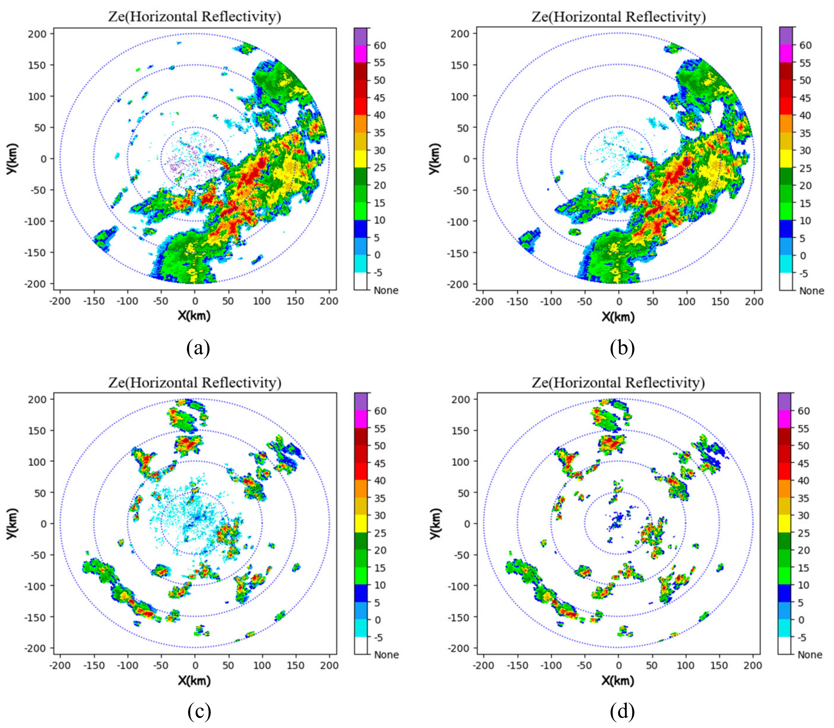
First, the experimental results of the noise and ground clutter filtering in data quality control are analyzed.

Figure 4 shows that after noise filtering, the noise points on the radar echo map become less and the edge of the echo map becomes smoother. After filtering ground clutter, the ground clutter located in the middle is filtered out, and the quality of the radar echo map is significantly improved.

To generate constant altitude plan position indicator (CAPPI) as the input of radar echo extrapolation methods, we employ three interpolation methods: linear interpolation in nearest neighbor combined with a vertical direction (NVI), linear interpolation in a vertical direction plus a horizontal direction (VHI) and linear interpolation of eight points (EPI). Figure 5 compares the original radar echo image and the interpolation results of the three interpolation methods.

Because the EPI interpolation method considers three factors: radial, azimuth and elevation, it can make more grid points get interpolated, and the EPI interpolation results are smoother. Therefore, the EPI interpolation method was used in the extrapolation experiments.

3. Deep Learning Algorithm

The first step of deep learning is the specification and quality of training data. The second step is the selection and optimization of the training algorithm, and the third step is the parameter setting, network depth and level matching of the training network. The configuration of each link has a great or small influence on the training effect. Therefore, in terms of the algorithm’s complexity, the deep learning algorithm takes it into account more comprehensively.

Based on deep learning theory, this section combines the CNN and LSTM neurons to form the Conv-LSTM neurons, which serve as the core and engine of neural network training. The Conv-LSTM is used as the neuron of the encoder–decoder model to form a time-series prediction model for radar echo extrapolation.

When training data in deep learning, the corresponding loss function should be selected as the optimization target of the optimization algorithm to gradually improve the convergence speed of the training. Different “tasks” of the network are implemented, and the loss functions selected are different. In this paper, mean square error ($MSE$) and other loss functions are used for the training optimization of deep learning. Experiments show that such loss functions can make the network achieve the best convergence effect. The flowchart of the proposed method by this paper is shown in Figure 6.

3.1. Conv-LSTM Neural Network

3.1.1. Convolutional Neural Network

CNN is a deep neural network with convolutional operation as its core idea [28]. Its three core technologies are receptive field, weight sharing and downsampling layer [29,30]. The structure of CNN generally includes an input layer, convolutional layer, excitation function, downsampling layer, full-connection layer and output layer.

For the convolution operation, the convolution kernel scan input, after matrix multiplication and overlaying the bias, can be used to calculate the value of the neuron at the next layer:

$$Z^{l+1}\left(i,j\right)=\left[Z^l\otimes w^{l+1}\right]\left(i,j\right)+b={\displaystyle \sum _{k=1}^{K_l}{\displaystyle \sum _{x=1}^f{\displaystyle \sum _{y=1}^f\left[Z_k^l\left(s_{0}i+x,s_{0}j+y\right)w_k^{l+1}\left(x,y\right)\right]}}}$$

(6)

$$\left(i,j\right)\in \left\{0,1,\dots L_{l+1}\right\}{ \mathrm{L}}_{l+1}=\frac{L_1+2p-f}{s_0}+1$$

(7)

In Equations (6) and (7), $Z^l$ and $Z^{l+1}$ represent the input and output of the $l+1$ layer and $L_{l+1}$ is the size of $Z^{l+1}$. It is assumed that the feature graphs have the same length and width.

$Z\left(i,j\right)$ is the pixel of the feature graph; $K$ is the number of channels of the feature graph; $f$ is the side length of the square convolution kernel; $s_0$ is the step length of the convolution kernel movement; and $p$ is the size of filling in 0 during the convolution.

When $f=1$, $s_0=1$ and $p=0$, the convolution operation using the cross-correlation algorithm is equivalent to the full join operation:

$$Z^{l+1}={\displaystyle \sum _{k=1}^{K_l}{\displaystyle \sum _{i=1}^L{\displaystyle \sum _{j=1}^L\left(Z_{i,j,k}^l{w}_k^{l+1}\right)+b=w_{l+1}^T{Z}_{l+1}+b,\hspace{1em}{L}^{l+1}=L}}}$$

(8)

The convolution and downsampling operations are shown in Figure 7. In Figure 7, $\ast$ represents the convolution operation.

The hidden and output layers, or the hidden and hidden layers are connected through the excitation function, called the excitation function relationship. The most common excitation functions for deep learning include the Sigmoid, Tanh, Maxsoft and ReLU functions. The first two excitation functions belong to the nonlinear rectifier function. The last one belongs to the linear rectifier function, which is also the most commonly used one of the excitation functions.

3.1.2. LSTM Neural Network

The recurrent neural network (RNN) is mainly used in time-series prediction. Its most obvious feature is that the output of the neuron at a certain moment can be fed into the neuron again as the input, meaning that the data at the previous and next moments can produce correlation and dependence. This is why RNN is applied to time series. For multi-layer RNN, there are only three weight parameters to be calculated for each layer. Because weight parameters are shared globally such as CNN, the number of hyperparameters to be calculated for RNN is significantly reduced.

The disadvantage of RNN is also very obvious. If the predicted time is very long, the increase or decrease in the loss value is too severe, leading to the problem of gradient vanishing and extinction [31].

To solve the problem of gradient explosion and disappearance generated by the RNN neural network for long-time prediction, LSTM was built and extended on this basis. LSTM is an upgraded version of RNN invented by Jürgen Schmidhuber in 1997 [32]. It has been proved to have an excellent ability to deal with long sequence problems [33]. The structure of LSTM is shown in Figure 8.

The core idea of LSTM is to preserve and perpetuate long-time cell states. Additionally, three “gate switches” are designed to control the weight change of cell and neuron states at each moment. The three “gate switches” include the forgetting, input and output gates. The equations of LSTM are as follows:

$$\begin{array}{l}{i}_t=sigmoid(W_{xi}{x}_t+W_{hi}{h}_{t-1}+W_{ci}{c}_{t-1}+b_i)\hfill \\ f_t=sigmoid(W_{xf}{x}_t+W_{hf}{h}_{t-1}+W_{cf}{c}_{t-1}+b_f)\hfill \\ c_t=c_{t-1}\circ f_t+i_t\circ \tanh \left(W_{xc}{x}_t+W_{hc}{h}_{t-1}+b_c\right)\hfill \\ o_t=sigmoid(W_{xo}{x}_t+W_{ho}{h}_{t-1}+W_{co}\circ c_t+b_o)\hfill \\ h_t=o_t\circ \tanh \left(c_t\right)\hfill \end{array}$$

(9)

Here, $\circ$ represents the Hadamard product; $i_t$ represents the input at the current moment; $W$ represents the weight matrix; $b$ represents the bias; $c_{t-1}$ represents the state at the previous moment; $f_t$ represents the value of the forgetting gate (i.e., which cell state should be forgotten); $c_t$ represents the state at the current moment; $o_t$ represents the output at the current moment; and $h_t$ represents the final output after the Hadamard product of the current output and state.

3.1.3. Conv-LSTM Neural Network

The classical LSTM structure expands the data into one dimension for prediction, which can better solve the time correlation. However, FC-LSTM can only extract the time-series information but cannot extract the spatial information. Spatial data, especially the radar echo data, contain much redundant information that cannot be processed by FC-LSTM.

To solve this problem, a convolution structure between input-to-state and state-to-state arises at the historic moment. Conv-LSTM uses convolution instead of full connection to extract the spatial information of sequence. In other words, the main difference between FC-LSTM and Conv-LSTM is that Conv-LSTM replaces matrix multiplication operation with convolution operation. The equations are as follows:

$$\begin{array}{l}{i}_t=sigmoid\left(W_{xi}\ast x_t+W_{hi}\ast h_{t-1}+W_{ci}\circ c_{t-1}+b_i\right)\hfill \\ f_t=sigmoid(W_{xf}\ast x_t+W_{hf}\ast h_{t-1}+W_{cf}\circ c_{t-1}+b_f)\hfill \\ c_t=c_{t-1}\circ f_t+i_t\circ \tanh \left(W_{xc}\ast x_t+W_{hc}\ast h_{t-1}+b_c\right)\hfill \\ o_t=sigmoid\left(W_{xo}\ast x_t+W_{ho}\ast h_{t-1}+W_{co}\circ c_t+b_o\right)\hfill \\ h_t=o_t\circ \tanh \left(c_t\right)\hfill \end{array}$$

(10)

where $*$ represents the convolution operation.

3.2. Encoder–Decoder Model

The reason for adopting the encoder–decoder model is the asymmetry of input and output. Applying this model, inputs of different lengths can be used to calculate outputs of different lengths, which solves the disadvantage that LSTM must have input and output symmetry. The basic idea is to use two batches of RNN, one batch of RNN as encoder and the other batch of RNN as the decoder. The encoder and decoder should ensure asymmetrical structure too.

The input of the encoder of the deep learning neural network model is the radar echo data. After multi-layer downsampling and convolutional layer processing, the cell state is packaged and sent to the decoder. The decoder takes the cell state as the input and restores the cell state to a specific output data through a multi-layer of deconvolution and upsampling. Figure 9 shows structure of the encoder–decoder model.

In this paper, we used three Conv-LSTM as encoder and three Conv-LSTM as decoder. Then, add downsampling and upsampling into the encoder and decoder separately. The downsampling and upsampling are implemented in convolution and deconvolution, respectively.

3.3. Loss Function

When training data in deep learning, the corresponding loss function should be selected as the optimization target of the optimization algorithm to gradually improve the performance of the dataset. The appropriate loss function can make the network achieve the best convergence effect.

The radar echo extrapolation in this paper belongs to the machine learning regression model. The regression model is supervised learning used to predict the numerical target value and make an approximate prediction of the real value. The regression model is a supervised learning algorithm, meaning that the predicted data are continuously distributed.

The evaluation criterion of deep learning for good or bad results is the loss function. The smaller the value of the loss function, the better the performance and robustness of the model. For the regression problem, the output should be continuous. Therefore, the loss function of the neural network can choose $MSE$, mean absolute error ($MAE$) and root mean square error ($RMSE$). Their corresponding calculation methods are shown in Equations (11)–(13). These loss functions have similar properties. They are all calculated based on a matrix “point-to-point”, allowing one to visually see the similarities between predicted and true values. In this paper, $MSE$ is chosen as the loss function.

$$MSE=\frac{1}{M}{\displaystyle \sum }_{i=1}^M{\left({\widehat{y}}_i-y_i\right)}^2$$

(11)

$$MAE=\frac{1}{M}{\displaystyle \sum }_{i=1}^M\left|{\widehat{y}}_i-y_i\right|$$

(12)

$$RMSE=\sqrt{\frac{1}{M}{\displaystyle \sum }_{i=1}^M{\left({\widehat{y}}_i-y_i\right)}^2}$$

(13)

We adopted a weight matrix to measure the importance of the reflectivity factor value because the occurrence probability of low reflectivity factor value is very high, and the higher the reflectivity factor value, the lower the occurrence probability.

$$w\left(x\right)=\left\{\begin{array}{l}1, x<15\hfill \\ 5, 15\le x<30\hfill \\ 10, 30\le x\le 40\hfill \\ 30, x>40\hfill \end{array}\right.$$

(14)

In Equation (9), x represents the value of the reflectivity factor. Its unit is $\mathrm{dBZ}$.

4. Evaluation Criteria of Extrapolation Results

For the test of precipitation forecast, it is generally divided into two classes.

The first class is the matrix “point-to-point” test method. This method uses “point-to-point” method to calculate the difference between two matrices of the same size, and then obtain the mean value of all the differences. It allows us to visually see the difference between the two matrices from statistics. The representative methods of this class include $POD$, $CSI$ and $FAR$.

The second class is the space inspection technology. The traditional test method, matrix point-to-point test method, is easy to lead to the phenomenon of double punishment. It prefers to regard the precipitation forecast as a failed forecast. To overcome and eliminate this phenomenon, a space-based verification technology has been developed in recent years and applied to the evaluation of precipitation forecast. This technology can evaluate the prediction results from another angle, make the verification method more comprehensive and detailed.

4.1. Matrix “Point-to-Point” Test Method

$POD$, $CSI$ and $FAR$ are calculated by the binary confusion matrix. The matrix contains four values: true positive ($TP$), false negative ($FN$), false positive ($FP$) and true negative ($TN$). The standard evaluation needs to set a threshold to evaluate whether the real value and the predicted value meet the same conditions and can be evaluated as different results. The definitions of these values are shown in

Table 1. Binary confusion matrix.

	Prediction Is Positive	Prediction Is Negative
Observation is positive	$TP$	$FN$
Observation is negative	$FP$	$TN$

.

For example, the weather radar echo extrapolation needs to set the threshold of reflectivity factor in $\mathrm{dBZ}$. $TP$ represents the number of points both observed and predicted to be greater than the threshold, $FN$ represents the number of points observed to be greater than the threshold but predicted to be less than the threshold, $FP$ represents the number of points observed to be less than the threshold but predicted to be greater than the threshold and $TN$ represents the number of points both observed and predicted to be less than the threshold.

For $POD$, $CSI$ and $FAR$, their equations are as follows:

$$\left\{\begin{array}{c}POD=\frac{TP}{TP+FN}\\ FAR=\frac{FP}{TP+FP}\\ CSI=\frac{TP}{TP+FN+FP}\end{array}\right.$$

(15)

4.2. Spatial Test Method

The calculation process of CRA is to select the observation area to be evaluated and then find the corresponding area on the predicted precipitation map. The error in these two areas is called the error before displacement. Then, the predicted precipitation map is shifted to a certain angle. When the error between the predicted precipitation map and the observed precipitation map reaches the minimum, the mean square error is the translation error. The area of the predicted area, plus the area where the predicted precipitation map and the observed precipitation map reaches the minimum, plus the area of the observed data are called the CRA verification area.

The error of precipitation forecast can be divided into three parts: displacement error, intensity error and shape error:

$$\begin{array}{c}MS{E}_{total}=MS{E}_{displacement}+MS{E}_{volume}+MS{E}_{pattern}\\ MS{E}_{total}=\frac{1}{N}{\displaystyle \sum _{i=1}^N}{\left(f_i-O_i\right)}^2\end{array}$$

(16)

In the above equations, $f_i$ and $O_i$ represent the prediction and observation results in the CRA verification area and $N$ represents the number of data points compared.

$$MS{E}_{displacement}=MS{E}_{total}-MS{E}_{shift}$$

(17)

where $MS{E}_{shift}$ is the translation error. It is obtained by the following equation:

$$MS{E}_{shift}=\frac{1}{N}{\displaystyle \sum _{i=1}^N{\left(f_i{}^{\prime }-o_i\right)}^2}$$

(18)

The volume error is calculated by subtracting the average observation result after displacement from the average prediction result after displacement:

$$MS{E}_{volume}={\left({\overline{f}}^{\prime }-\overline{o}\right)}^2$$

(19)

Finally, the pattern error is obtained by subtracting the volume error from the translation error:

$$MS{E}_{pattern}=MS{E}_{shift}-MS{E}_{volume}$$

(20)

5. Experiment Results Analysis

5.1. CTREC Algorithm

Figure 10 shows the results of the test set extrapolation of the CTREC algorithm, demonstrating the extrapolation results at four moments.

We used two different evaluation algorithms to evaluate the test set, and the evaluation results are presented in

Table 2. CTREC algorithm extrapolation results at 0.5 h.

$\mathbf{Echo} \mathbf{Threshold} \left(\mathbf{d}\mathbf{B}\mathbf{Z}\right)$	$\mathit{P}\mathit{O}\mathit{D}$	$\mathit{C}\mathit{S}\mathit{I}$	$\mathit{F}\mathit{A}\mathit{R}$
10	0.87	0.87	0.10
20	0.80	0.77	0.30
30	0.63	0.51	0.27
40	0.17	0.08	0.86

,

Table 3. CTREC algorithm extrapolation results at 1 h.

$\mathbf{Echo} \mathbf{Threshold} \left(\mathbf{d}\mathbf{B}\mathbf{Z}\right)$	$\mathit{P}\mathit{O}\mathit{D}$	$\mathit{C}\mathit{S}\mathit{I}$	$\mathit{F}\mathit{A}\mathit{R}$
10	0.83	0.82	0.17
20	0.80	0.75	0.35
30	0.42	0.28	0.58
40	0.20	0.15	0.88

and

Table 4. CTREC algorithm extrapolation results’ CRA score.

	Categories	Percent Displacement	Percent Pattern	Percent Volume	Total MSE
Time
0.5 h		0.08	0.82	0.08	2.99
1 h		0.72	0.62	0.20	3.26

. Here, we selected 10, 20, 30 and 40 $\mathrm{dBZ}$ as echo thresholds because they are the boundary values of distinguishing light rain (between 10 and 20 $\mathrm{dBZ}$), moderate rain (between 20 and 30 $\mathrm{dBZ}$), heavy rain (between 30 and 40 $\mathrm{dBZ}$) and torrential rain (greater than 40 $\mathrm{dBZ}$).

As presented in Table 2 and Table 3, the higher the $POD$ and $CSI$, the better the extrapolation results, and the lower the $FAR$, the better the extrapolation results. As shown in Table 4, the total MSE manifests the performance of the extrapolation results from another perspective. The percent displacement, percent pattern and percent volume mean to judge the results in three aspects, and the smaller the total MSE, the better the extrapolation results.

5.2. TITAN Algorithm

As shown in Figure 11, the ellipses on (a) and (b) are storm cells with a reflectivity factor greater than 30 $\mathrm{dBZ}$. The time interval between the two images is 6 min; it can be seen that the number of cells in the two echoes is different.

The phenomenon of division, merger, extinction and generation of the cells can be seen in the radar echo cells identified at each moment in Figure 11 and Figure 12. To accurately track and predict the cells, appropriate judgment conditions and restrictive conditions need to be added.

Therefore, we used the radar echo images of the first six moments to carry out the least square fitting method to obtain the development process of different cells. Additionally, a representative monomer prediction process is selected for analysis, as shown in Figure 13 and Figure 14.

The predicted evaluation results are presented in

Table 5. TITAN algorithm extrapolation results at the threshold of 30 $\mathrm{dBZ}$.

Extrapolation Time (min)	$\mathit{P}\mathit{O}\mathit{D}$	$\mathit{C}\mathit{S}\mathit{I}$	$\mathit{F}\mathit{A}\mathit{R}$
12	0.71	0.65	0.18
30	0.62	0.50	0.34
42	0.55	0.46	0.50
60	0.30	0.24	0.71

and

Table 6. TITAN algorithm extrapolation results’ CRA score.

	Categories	Percent Displacement	Percent Pattern	Percent Volume	Total MSE
Time
0.5 h		0.19	0.62	0.19	2.73
1 h		0.23	0.69	0.08	3.05

.

5.3. Deep Learning Algorithm

Figure 15 shows the results of the deep learning algorithm test set extrapolation, demonstrating the extrapolation results at four moments. Two different evaluation algorithms were used to evaluate the test set and the evaluation results are presented in

Table 7. Deep learning algorithm extrapolation results at 0.5 h.

$\mathbf{Echo} \mathbf{Threshold} \left(\mathbf{d}\mathbf{B}\mathbf{Z}\right)$	$\mathit{P}\mathit{O}\mathit{D}$	$\mathit{C}\mathit{S}\mathit{I}$	$\mathit{F}\mathit{A}\mathit{R}$
10	0.88	0.83	0.05
20	0.77	0.75	0.26
30	0.67	0.56	0.31
40	0.30	0.20	0.75

,

Table 8. Deep learning algorithm extrapolation results at 1 h.

$\mathbf{Echo} \mathbf{Threshold} \left(\mathbf{d}\mathbf{B}\mathbf{Z}\right)$	$\mathit{P}\mathit{O}\mathit{D}$	$\mathit{C}\mathit{S}\mathit{I}$	$\mathit{F}\mathit{A}\mathit{R}$
10	0.80	0.75	0.10
20	0.75	0.72	0.23
30	0.60	0.42	0.51
40	0.25	0.18	0.83

and

Table 9. Deep learning algorithm CRA score.

	Categories	Percent Displacement	Percent Pattern	Percent Volume	Total MSE
Time
0.5 h		0.09	0.39	0.52	1.15
1 h		0.02	0.92	0.07	1.35

.

6. Conclusions and Prospects

As an important means of near weather forecasting technology, this paper focused on the extrapolation algorithm and exploration in the meteorological field, which is worthy of further improvement and perfection. Our proposed extrapolation method of deep learning takes the reflectivity factor data in the Doppler weather radar base data as the input. Before feeding it into the neural network, we conducted several preprocessing operations on the data for training so that the input data could meet the requirements of training. The data preprocessing is essential and the effect of the training is significantly improved after the data are preprocessed.

The deep learning algorithm has achieved good results under the set threshold and prediction time range. Multiple table data demonstrate the advantages of the proposed method by this paper.

For the matrix “point-to-point” test method, under the threshold of 10 $\mathrm{dBZ}$ or 20 $\mathrm{dBZ}$, whether at the time of 0.5 h or 1 h, the $POD$, $CSI$ and $FAR$ of the deep learning algorithm have tiny differences compared with the CTREC algorithm. The reason for this phenomenon is that radar echo with low $\mathrm{dBZ}$ is easy to forecast. However, under the threshold of 30 $\mathrm{dBZ}$ and 40 $\mathrm{dBZ}$, at the time of 0.5 h, the $POD$, $CSI$ and $FAR$ of the deep learning algorithm are 0.67, 0.56, 0.31 and 0.30, 0.20, 0.75, compared with 0.63, 0.51, 0.27 and 0.17, 0.08 and 0.86 for the CTREC algorithm, and 0.62, 0.50 and 0.34 for the TITAN algorithm. Meanwhile, under the threshold of 30 $\mathrm{dBZ}$ and 40 $\mathrm{dBZ}$, at the time of 1 h, the $POD$, $CSI$ and $FAR$ of the deep learning algorithm are 0.60, 0.42, 0.51 and 0.25, 0.18 and 0.83, compared with 0.42, 0.28, 0.58 and 0.20, 0.15 and 0.88 for the CTREC algorithm and 0.30, 0.24 and 0.71 for the TITAN algorithm. Therefore, we can conclude that the accuracy of the deep learning algorithm is obviously higher than the CTREC algorithm and TITAN algorithm.

For the spatial test method, at the time of 0.5 h and 1 h, the MSE total of the deep learning algorithm is 1.15 and 1.35 compared with 2.99 and 3.26 for the CTREC algorithm and 2.73 and 3.05 for the TITAN algorithm. Consequently, the stability of the deep learning algorithm is better than the CTREC and TITAN algorithms. We can obtain this conclusion from these figures as well. For example, for CTREC algorithm extrapolation results in Figure 10, the figures (d), (f) and (h) can approve that at the time of 30 min, 42 min and 60 min, the shapes of the extrapolation results change a lot from the observations. For the TITAN algorithm extrapolation results in Figure 13 and Figure 14, the extrapolation results also change somewhat. However, for the deep learning algorithm extrapolation results in Figure 15, the figures (d), (f) and (h) can approve that at the time of 30 min, 42 min and 60 min, the shapes of the extrapolation results change a little.

From experiments results, it is confirmed that both in statistic and morphology the proposed method by this paper is superior to traditional radar echo extrapolation methods, CTREC and TITAN algorithms.

Additionally, compared with the CTREC algorithm, the extrapolation results of the deep learning algorithm are continuous, having no discrete points, which is significant for the judgment and measurement of the precipitation area. Compared with the TITAN algorithm, the deep learning algorithm can not only extrapolate the low-intensity echo region, but it also has a better accuracy of the high-intensity echo region. Furthermore, the deep learning algorithm can respond to the disappearance and generation of echoes in time, which makes it quickly respond to severe convective weather. Through the training, learning and feature extraction of massive data, the deep learning extrapolation algorithm forms a system that can automatically solve the inherent law of the data and predict the development trend of the data. This is of great help to the landing of precipitation forecast and make it business-oriented.

References

- Yu, X.; Zhou, X.; Wang, X. The advances in the nowcasting techniques on thunderstorms and severe convection. Acta Meteorol. Sin. 2012, 70, 311–337. [Google Scholar] [CrossRef]
- Chen, M.; Yu, X.; Tan, X. A brief review on the development of nowcasting for convective storms. J. Appl. Meteor. Sci. 2004, 15, 754–766. [Google Scholar]
- Cheng, C.; Chen, M.; Wang, J.; Gao, F.; Yeung Linus, H.Y. Short-term quantitative precipitation forecast experiments based on blending of nowcasting with numerical weather prediction. Acta Meteorol. Sin. 2013, 71, 397–415. [Google Scholar] [CrossRef]
- Chen, M.; Bica, B.; Tüchler, L.; Kann, A.; Wang, Y. Statistically Extrapolated Nowcasting of Summertime Precipitation over the Eastern Alps. Adv. Atmos. Sci. 2017, 34, 925–938. [Google Scholar] [CrossRef]
- Wilson, J.; Pierce, C.; Seed, A. Sydney 2000 Field Demonstration Project–Convective storm nowcasting. Weather Forecast. 2004, 19, 131–150. [Google Scholar] [CrossRef]
- Li, P.W.; Lai, E. Applications of radar-based nowcasting techniques for mesoscale weather forecasting in Hong Kong. Meteorol. Appl. 2010, 11, 253–264. [Google Scholar] [CrossRef] [Green Version]
- Cao, C.; Chen, Y.; Liu, D.; Li, C.; Li, H.; He, J. The optical flow method and its application to nowcasting. Acta Meteorol. Sin. 2015, 73, 471–480. [Google Scholar] [CrossRef]
- Han, L.; Wang, H.; Tan, X.; Lin, Y. Review on Development of Radar based Storm Identification, Tracking and Forecasting. Meteor Mon. 2007, 33, 3–10. [Google Scholar]
- Noel, T.M.; Fleisher, A. The Linear Predictability of Weather Radar Signals; Massachusetts Inst of Tech Cambridge: Cambridge, MA, USA, 1960; 46p. [Google Scholar]
- Hilst, G.R.; Russo, J.A. An Objective Extrapolation Technique for Semi-Conservative Fields with an Application to Radar Patterns; The Travelers Research Center: Hartford, CT, USA, 1960; 34p. [Google Scholar]
- Kessler; Russo, J.A. Statistical Properties of Weather Radar Echoes. In Proceedings of the 10th Weather Radar Conference, Washington, DC, USA, 22–25 April 1963; pp. 25–33. [Google Scholar]
- Kessler, E. Computer Program for Calculating Average Lengths of Weather Radar Echoes and Pattern Bandedness. J. Atmos. Sci. 1966, 23, 569–574. [Google Scholar] [CrossRef] [Green Version]
- Barclay, P.A.; Wilk, K.E. Severe thunderstorm radar echo motion and related weather events hazardous to aviation operations. ESSA Tech. Memo. 1970, 46, 63. [Google Scholar]
- Wilk, K.E.; Gray, K.C. Processing and analysis techniques used with the NSSL weather radar system. In Proceedings of the 14th Conference on Radar Meteorology, Tucson, AZ, USA, 17–20 November 1970; pp. 369–374. [Google Scholar]
- Dixon, M.; Wiener, G. TITAN: Thunderstorm Identification, Tracking, Analysis, and Nowcasting-A Radar-based Methodology. J. Atmos. Ocean. Technol. 1993, 10, 785. [Google Scholar] [CrossRef]
- Johnson, J.T.; MacKeen, P.L.; Witt, A.; Mitchell, E.D.W.; Stumpf, G.J.; Eilts, M.D.; Thomas, K.W. The Storm Cell Identification and Tracking Algorithm: An Enhanced WSR-88D Algorithm. Weather Forecast. 1998, 13, 263–276. [Google Scholar] [CrossRef] [Green Version]
- Chen, X. Research on Optimization of Deep Learning Algorithm Based on Convolutional Neural Network; Zhejiang Gongshang University: Hangzhou, China, 2014. [Google Scholar]
- Lecun, Y.; Bengio, Y.; Hinton, G. Deep learning. Nature 2015, 521, 436. [Google Scholar] [CrossRef] [PubMed]
- Klein, B.; Wolf, L.; Afek, Y. A Dynamic Convolutional Layer for short range weather prediction. In Proceedings of the IEEE Conference on Computer Vision and Pattern Recognition, Boston, MA, USA, 7–12 June 2015; pp. 4840–4848. [Google Scholar]
- Jing, J.; Li, Q.; Peng, X.; Ma, Q.; Tang, S. HPRNN: A Hierarchical Sequence Prediction Model for Long-Term Weather Radar Echo Extrapolation. In Proceedings of the IEEE International Conference on Acoustics, Speech and Signal Processing (ICASSP), Barcelona, Spain, 4–8 May 2020; pp. 4142–4146. [Google Scholar]
- Guo, S.Z.; Xiao, D.; Yuan, H.Y. A Short-term rainfall prediction method based on neural networks and model ensemble. Adv. Meteor. Sci. Technol 2017, 7, 107–113. [Google Scholar]
- Shao, Y.H.; Zhang, W.C.; Liu, Y.H.; Sun, C.W.; Fu, C.Y. Application of Back-Propagation Neural Network in Precipitation Estimation with Doppler Radar. Plateau Meteorol. 2009, 28, 846–853. [Google Scholar]
- Shi, E.; Li, Q.; Gu, D.; Zhao, Z. Weather radar echo extrapolation method based on convolutional neural networks. J. Comput. Appl. 2018, 38, 661–665. [Google Scholar]
- Kumjian, M.R. Principles and Applications of Dual-Polarization Weather Radar. Part I: Description of the Polarimetric Radar Variables. J. Oper. Meteorol. 2013, 1, 226–242. [Google Scholar] [CrossRef]
- Doviak, R.; Zrnic, S. Doppler Radar and Weather Observations; Dover Publications: Norman, OK, USA, 2006. [Google Scholar]
- Kou, L.L.; Chao, L.Y.; Chu, Z.G. C-Band Dual-Polarization Doppler Weather Radar Data Analysis and Its Application in Quantitative Precipitation Estimation. J. Trop. Meteorol. 2018, 4, 30–41. [Google Scholar]
- Zhang, J.; Wang, S.; Clarke, B. WSR-88D reflectivity quality control using horizontal and vertical reflectivity structure. In Proceedings of the 11th Conference Aviation, Range, and Aerospace Meteor, Hyannis, MA, USA, 3–8 October 2004. [Google Scholar]
- Lecun, Y.; Bottou, L. Gradient-based learning applied to document recognition. Proc. IEEE 1998, 86, 2278–2324. [Google Scholar] [CrossRef] [Green Version]
- Hubel, D.H.; Wiesel, T.N. Receptive fields, binocular interaction and functional architecture in the cat’s visual cortex. J. Physiol. 1962, 160, 106–154. [Google Scholar] [CrossRef]
- Fukushima, K. Neocognitron: A self-organizing neural network model for a mechanism of pattern recognition unaffected by shift in position. Biol. Cybern. 1980, 36, 193–202. [Google Scholar] [CrossRef] [PubMed]
- Jozefowicz, R.; Zaremba, W.; Sutskever, I. An Empirical Exploration of Recurrent Network Architectures. In Proceedings of the International Conference on International Conference on Machine Learning, Lille, France, 6–11 July 2015. [Google Scholar]
- Hochreiter, S.; Schmidhuber, J. Long Short-Term Memory. Neural Comput. 1997, 9, 1735–1780. [Google Scholar] [CrossRef] [PubMed]
- Pascanu, R.; Mikolov, T.; Bengio, Y. On the difficulty of training Recurrent Neural Networks. In Proceedings of the 30th International Conference on Machine Learning, Atlanta, GA, USA, 16–21 June 2013; Volume 28, pp. 1310–1318. [Google Scholar]
Figure 1.
Flowchart of data preprocessing.
Figure 2.
Window centered on the database.
Figure 3.
Schematic of the eight-point interpolation method.
Figure 4.
Noise filtering effect in
Figure 2 ((
a) represents the original echo image; (
b) represents the echo image after noise filtering; (
c) represents the original echo image; (
d) represents the echo image after ground object clutter filtering).
Figure 5.
Interpolation results 1 ((a) represents PPI; (b) represents NVI interpolation results; (c) represents VHI interpolation results; (d) represents EPI interpolation results).
Figure 6.
Flowchart of the proposed method by this paper.
Figure 7.
Schematic of the convolution and downsampling operation ((a) is the convolution operation and (b) is downsampling operation).
Figure 8.
Schematic of the LSTM neuron structure.
Figure 9.
Schematic of the encoder-decoder model.
Figure 10.
Comparison between the extrapolation results of the CTREC algorithm at 0.5 h and the actual situation ((a) 00:18 actual situation, (b) 00:18 extrapolation, (c) 00:30 actual situation, (d) 00:30 extrapolation, (e) 00:42 reality, (f) 00:42 extrapolation, (g) 00:60 reality and (h) 00:60 extrapolation).
Figure 11.
(a) TITAN algorithm recognition result at t3 and (b) TITAN algorithm recognition result at t4.
Figure 12.
Figure 13.
(a) Actual position of the monomer at 0.5 h and (b) predicted position of the monomer at 0.5 h.
Figure 14.
(a) Actual position of the monomer at 1 h and (b) predicted position of the monomer at 1 h.
Figure 15.
Comparison between extrapolation results and reality at 0.5 h of the deep learning algorithm ((a) 00:18 reality, (b) 00:18 extrapolation, (c) 00:30 reality, (d) 00:30 extrapolation, (e) 00:42 reality, (f) 00:42 extrapolation, (g) 00:60 reality and (h) 00:60 extrapolation).