Interannual Variability of Summer Hotness in China: Synergistic Effect of Frequency and Intensity of High Temperature

Abstract

In the context of global warming, the impact of summer high temperature events is increasing. The accumulated summer high temperature is often used to reflect the overall hotness of summer. The internal variation of the accumulated temperature can be affected by both the frequency and intensity. In this study, by using the daily data during summers of 1960–2018, we examine the relative importance of the two factors with a multiple linear regression method. It is demonstrated that that the dominant result of summer accumulated temperature is sensitive to the change of threshold. As the threshold increases, the importance of frequency gradually increases, while the importance of the intensity decreases. In addition, it is found that when the threshold changes, the sensitivity of the dominant results is different over regions. This can provide a basis for the selection of regional thresholds and further improve the representation of accumulated temperature for high summer temperatures.

1. Introduction

It was pointed out in the Sixth Assessment Report of the Intergovernmental Panel on Climate Change (IPCC AR6) that the global climate has shown a warming trend, and the trend will further intensify in the future [1,2,3]. Due to natural climate changes and human activities, large-scale climate anomalies occur frequently [4], and the frequency and intensity of high temperatures are increasing globally [5,6]. China is a sensitive region affected by climate change. A lot of research noted that, in China, the frequency and intensity of summer high temperature events had shown an increasing trend [7,8,9,10,11,12,13,14,15,16,17,18,19,20,21,22,23]. The high temperature events in summer will continue to increase in the future [24,25].

The frequent occurrence of high temperatures in summer will have a great impact on human life and property. The most direct effect is to increase human morbidity and mortality, causing serious social and economic losses, and even threatening people’s lives in countries and regions with aging populations and rapid urbanization development [26,27,28,29,30,31,32,33,34,35,36,37,38]. In addition, persistent high temperatures can also put tremendous pressure on the summer electricity load, which can easily cause electrical fire events.

In order to take precautions against the increasing frequency of high temperature events, we need to pay more attention to the study of summer hotness. In the past, the magnitude of the heat index was often used to characterize the hotness of a summer. For different purposes, various high temperature indexes have been proposed. These indexes have different emphases, and they all have advantages and disadvantages in reflecting summer hotness. Among the various indices, the “above a threshold” indices reflect more comprehensive contents than the seasonal average and the daily maximum [19], among which the number of days above a threshold [11,17,19,23,24,39] and the accumulated temperature are commonly used.

In the past, accumulated temperature has been more widely used in the agricultural field, such as the impact of accumulated temperature on the key growth period of crops [40,41,42] and the evaluation of heat resources [43,44,45,46]. Accumulated temperature is also used to study the influence of summer temperature on electric load [47,48,49,50]. In addition, it is often used for ecological problems, as an important index, such as vegetation growth period [51,52,53]. It has gradually begun to be used in the field of meteorology. Zhou [54] took the accumulated temperature as one of the indicators for dividing the north-south temperature region of Qinling Mountains. Chen et al. [15] used it to study the variation characteristics of high temperature heat wave. Miu et al. [55] used it to analyze the change characteristics of summer temperature in Nanjing. In the study, the variation trend of accumulated temperature is consistent with the extreme maximum temperature and also echoes with the change of average temperature. In the past research, accumulated temperature only focuses on the temperature when it exceeds 0 ℃, 10 ℃, and 35 ℃. Improving the relevant research on accumulated temperature can deepen the understanding of it, which in turn can further improve the relevant research in meteorology, agriculture, electric power, and many other application sectors.

In addition to the accumulated temperature, the average summer temperature and the daily extreme maximum temperature in summer are also indices of the severity of the high temperature. In fact, these two indices are two special cases of accumulated temperature under different thresholds. An extreme example is, when the threshold is particularly low, the 92-day temperature in summer (June–August) can be higher than the threshold. Then, under this threshold, the accumulated temperature actually appears as the average summer temperature. Another extreme example is, when the threshold temperature is selected too high, only one or two days are selected, then the accumulated temperature under the threshold appears to be the extreme highest temperature in summer. Therefore, the accumulated temperature is a more appropriate index to reflect the severity of summer hotness. When the threshold is between the two extremes, the accumulated temperature can reflect the content of the two indices, days (frequency) and intensity.

By analyzing the definition of accumulated temperature, we found that its variation is determined by both frequency and intensity. The frequency can also be described as the number of days of high temperature. The relationship of accumulated temperature with the days and intensity can be an analogy to the relationship of the total amount of precipitation with the days and intensity of precipitation. It can also be analogous to the relationship of atmospheric pressure with air temperature and density. According to the definitions, the three quantities hold a non-linear relationship. Analyzing the dominance and the relative importance of two or more non-linear impact factors, on which scholars have done research in many aspects in the past [56,57,58]. The method used in Lu [59,60,61] is applied in this study to explore the relative importance of days and intensity in the variation of the accumulated temperature. In this method, the non-linear relationship may be simplified as a linear relationship, as long as the fitting result can pass the significance test. The method was also used to estimate the relative importance of the factors influencing the land surface energy balance [62].

In this study, we focus on the summer high temperature, but let the high temperature threshold start from a low value and give the results from different “high temperature” thresholds. The purpose of study is to analyze the relative importance of the number of days and intensity to the accumulated temperature with different thresholds, and to investigate how the results will change with the threshold.

2. Materials and Methods

2.1. Data

The observed data used in this study are the daily maximum temperature of the 768 stations and the daily precipitation data of 2419 stations in China, during the 59 years from 1960 to 2018, provided by the China National Meteorological Information Center. Quality control has been performed with the data to ensure the consistency and correctness of the station datasets.

The quality control of temperature data is as follows. For one station, when the missing days are 15 days or less in 92 days in summer, the temperature of those days is dealing with the average of the highest temperature in summer of the station. When the missing days exceed 15 days, the year is recorded as a missing year. When the number of missing years exceeds more than 30, the station is excluded in the calculation. The precipitation data were strictly quality combed through the special work of ground base data. A total of 220 stations with more days of missing measurements were excluded, the remaining 2219 stations were involved in the calculation.

We used the reanalysis data: the monthly mean surface direct shortwave radiation flue and total cloud cover from ERA5 (the fifth generation ECMWF reanalysis for the global climate and weather), during the 40 years from 1979 to 2018.

Station precipitation data, total cloud cover, and mean surface direct shortwave radiation flue were selected to investigate the regional differences of influence factors to summer accumulation temperature.

2.2. Methods

We use different thresholds (k) to define the accumulated temperature day. In this study, k ranges from 27 ℃ to 36 ℃. Those thresholds were conducted by using the summer temperature series of the national site for the calendar year. Only those days, whose daily maximum temperature is k ℃ or higher, are treated as high temperature day (D). Only the temperature of these high temperature days is used to calculate the accumulated temperature (Z) and the intensity (S):

$$Z={{\displaystyle \sum }}_{\mathrm{i}=0}^{\mathrm{n}}({\mathrm{T}}_{\mathrm{i}}-k),(k=27,\dots \dots ,36).$$

(1)

k is the accumulated temperature threshold, T_i is the daily maximum temperature of D.

In each summer of the station, there is a D and Z corresponding to each threshold k. Then, the averaged temperature intensity of those days can be calculated as S = Z/D.

Lu et al., (2016) analyzed the relative importance of frequency and intensity in precipitation to study their relative contribution to the interannual variation of precipitation. Based on this method, we attempt to analyze the relative importance of intensity and days in accumulated temperature under different thresholds, and how the relative importance changes with the threshold.

Summer accumulated temperature (Z) is affected by the number of days (D) and the intensity (S). Linear regression is as follows:

Z = aD + bS + c.

(2)

Equation (2) is selected to fit the relationship between the three, and the relative importance is evaluated. To be sound in statistics, the validation of the approximation needs to be verified with a significance test.

The coefficients a and b can be understood as the variation rate of Z with respect to D and S. The meaning of them can be expressed as a = |∂Z/∂D| and b = |∂Z/∂S|.

Meanwhile, we can use σ_D and σ_S, the standard deviations of D and S determined from the data, to reflect their respective interannual variability. The products of the variation rates and the corresponding variation are used to measure, respectively, the scales of the changes in Z induced by the variations of D and S. It can be defined as M_D ≡ a · σ_D and M_S ≡ b · σ_S.

The partial correlation of an independent variable with the dependent quantity implies that the influences from other independent variables have been eliminated. To better understand the implication of the M_D and M_S, we can express them in terms of the correlation coefficients. After deduction, the two measures can be written as ${\mathrm{M}}_{\mathrm{D}}=\frac{{\stackrel{\sim }{\mathrm{r}}}_{\mathrm{ZD}}}{1-{\mathrm{r}}_{\mathrm{DS}}^2}$ and ${\mathrm{M}}_{\mathrm{S}}=\frac{{\stackrel{\sim }{\mathrm{r}}}_{\mathrm{ZS}}}{1-{\mathrm{r}}_{\mathrm{DS}}^2}$, where ${\stackrel{\sim }{\mathrm{r}}}_{\mathrm{ZD}}={\mathrm{r}}_{\mathrm{ZD}}-{\mathrm{r}}_{\mathrm{ZS}}{\mathrm{r}}_{\mathrm{DS}}$ and ${\stackrel{\sim }{\mathrm{r}}}_{\mathrm{ZS}}={\mathrm{r}}_{\mathrm{ZS}}-{\mathrm{r}}_{\mathrm{ZD}}{\mathrm{r}}_{\mathrm{DS}}$ in which r_ZD is the coefficient of simple linear correlation between Z and D, r_ZS is the coefficient of correlation between Z and S, and r_DS is the coefficient of correlation between D and S. These suggest that what the measures M_D and M_S reflect are the partial correlations of Z with D and S. It is therefore more reasonable to use the measures defined than the simple correlations to estimate the relative importance of the variables.

In the process of calculation, because D and S are two different quantities, the effects of the two cannot be directly compared. Therefore, we choose the standardized data to be brought into the calculation. The standard deviation of them: σ_D = σ_S = 1, then M_D = a, M_S = b. The relative importance of the two variables thus can be judged by directly comparing the magnitudes of the coefficients a and b.

In the analysis of the effecting factors of Z, the method can be written as

F = ln (a/b),

(3)

where F < 0, i.e., a < b; when F > 0, i.e., a > b. For each station, there will be an F-value corresponding to each temperature threshold.

3. Results

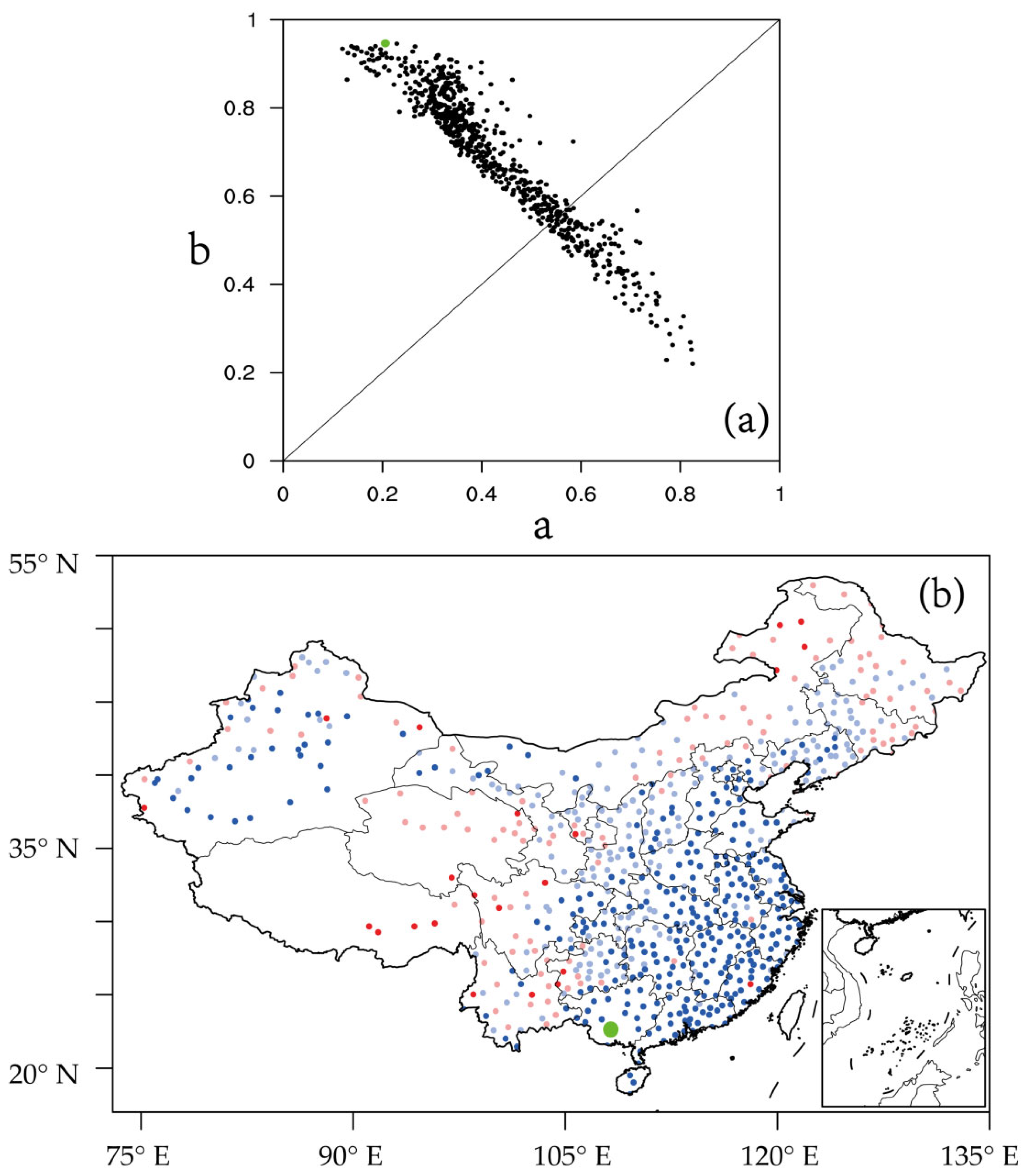
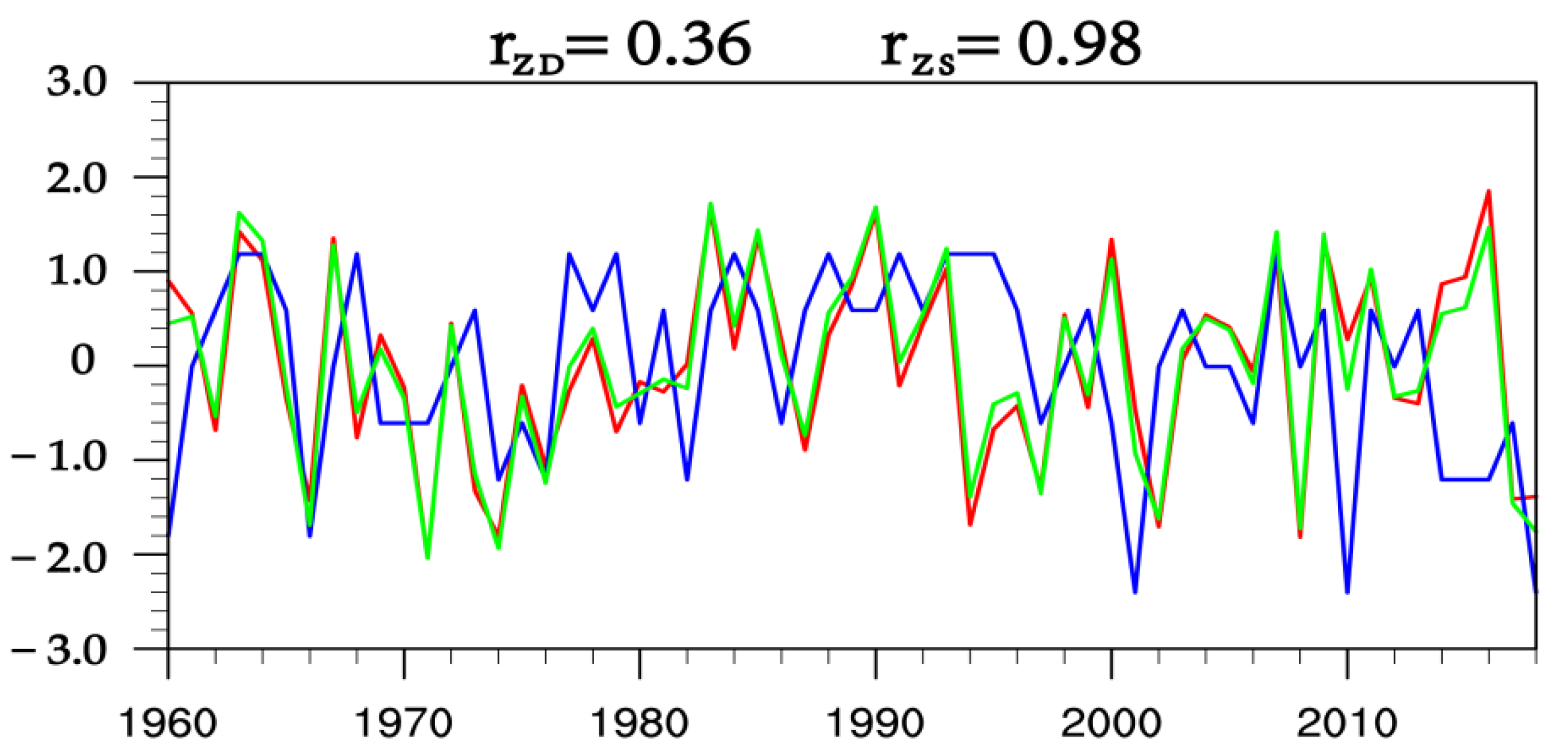
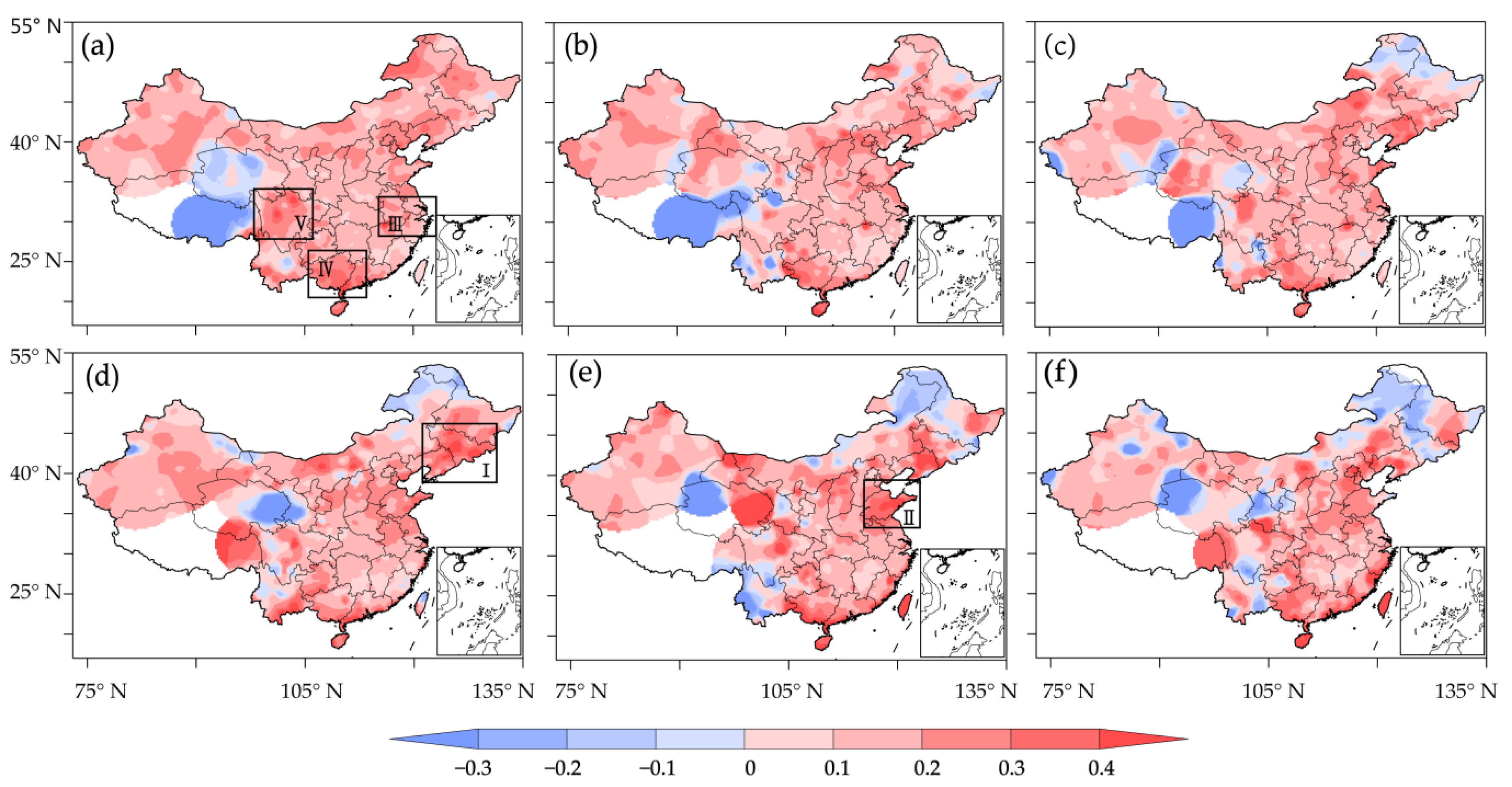
3.1. The Dominance for a Low Temperature Threshold

Figure 1a shows the relative importance of days and intensity of accumulated temperature when the threshold is 27 °C. Only stations which fitting results exceeding 95% significance level are shown. The distribution indicates that when the accumulated temperature is greatly affected by the intensity, it is less affected by the days. Under this threshold, most stations locate above the line of a = b, that is, b is larger than a. This suggests that for the threshold of 27 °C, the interannual variation of summertime accumulated temperature is more influenced by the intensity.

In this study, the magnitude of the coefficients a and b was used to express the relative importance of D and S on the summer accumulated temperature. For the analysis of the effecting factors of Z, Equation (3) was used. When F < 0, i.e., a < b, the main influence factor of accumulated temperature is the intensity, and the station is shown in blue in Figure 1b; when F > 0, i.e., a > b, the main influence factor is the days, and the station is shown in red. When a > 2b, that is, the influence of the days is much greater than the intensity, the variation of the accumulated temperature is considered to be dominated by the number of days. When b > 2a, the influence of the intensity is much greater than days, and the variation of the accumulated temperature is dominated by the intensity.

Figure 1b shows the main influence factor is either days or intensity of accumulated temperature. At the threshold of 27 °C, most stations are marked by blue, that is, the interannual variation of summer accumulated temperature at these stations is mainly determined by the intensity. The intensity is the main influencing factor. We found that in South China, East China, and some parts of Northwest China, the stations are dark blue, which means, these areas are affected mainly by intensity more than other areas. The regionality shows that, in the north-south direction, the impact of intensity to the accumulated temperature gradually decreases from south to north. Furthermore, in the east-west direction, the trend in high latitudes is opposite from that in mid-low latitudes. In mid-low latitudes, it shows a gradual decreasing trend from east to west, while the decreasing trend in mid-high latitudes is from east to west.

The station with the greatest relative influence of intensity on accumulated temperature, which is the green point in Figure 1, was selected. The interannual variation of accumulated temperature, days, and intensity was plotted.

As can be seen from the line in Figure 2, the variation of accumulated temperature and intensity is consistent, and the correlation between accumulated temperature and intensity is high. In this example, accumulated temperature and the days are also quite different. In addition, in comparison of Pearson’s r value, the result between accumulated temperature and days (r_ZD) is 0.36, while the coefficient between accumulated temperature and intensity (r_ZS) is 0.98. Both r_ZD and r_ZS are exceeded the significance level of 99%. That is, the correlation coefficient also enables to conclude that the intensity has a greater effect on the accumulated temperature at 27 °C.

The correlations are consistent with that drawn from the multiple linear regression. That is, the interannual variation of accumulated temperature at 27 °C is influenced by the days, but is mainly dominated by the intensity.

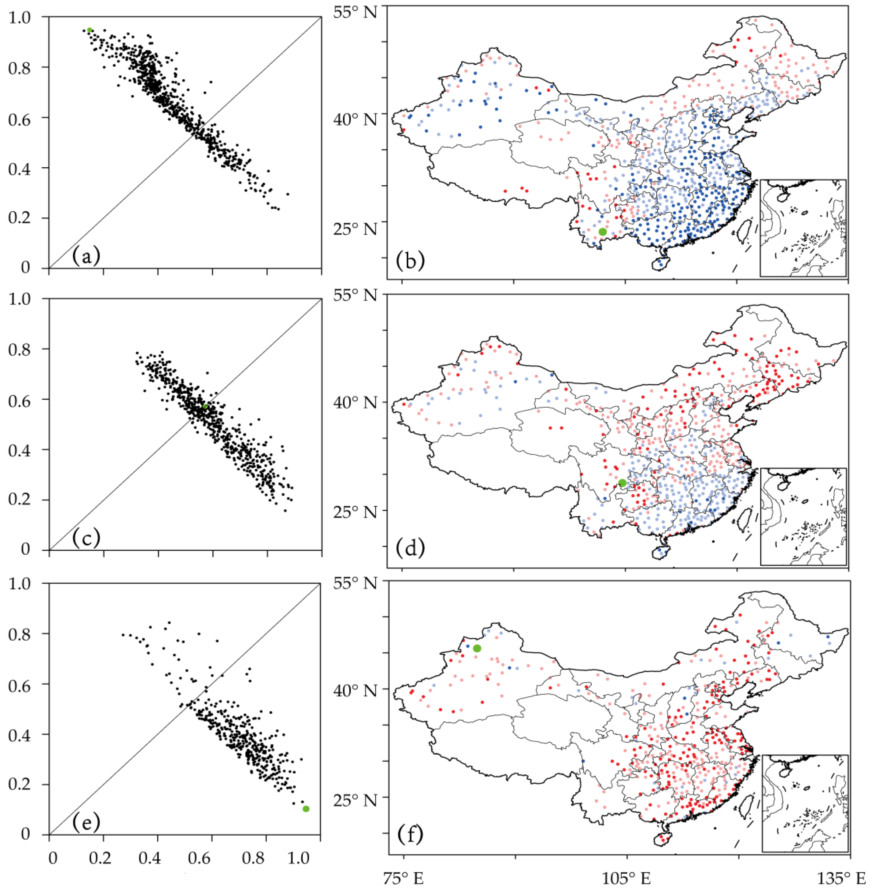
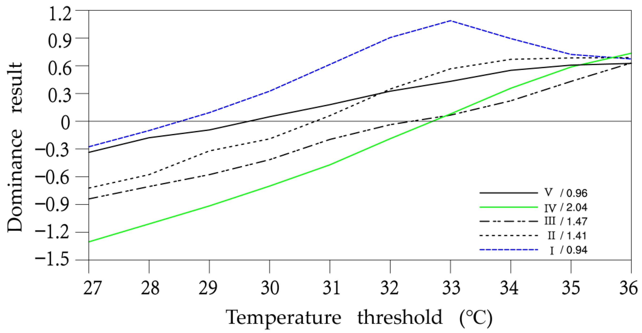
3.2. The Change of Dominance When Increasing Threshold

The magnitudes of accumulated temperature, days, and intensity in summer are closely related to the selection of threshold. In studying the relative effects of day and intensity on accumulated temperature, the effect will change with threshold. In this section, the threshold is increased from 28 °C to 36 °C, of which 28 °C, 32 °C, and 36 °C are selected as examples, as shown in Figure 3.

With the increase of the threshold, the scatter points in Figure 3a,c,e have a tendency to move along the a = b line, toward the lower right corner. The coefficient a steadily increases, while the coefficient b steadily decreases, indicating that the relative influence of the days gradually increases, while the relative influence of the intensity gradually decreases. Comparing Figure 3b,d,f, it is found that, in the process of increasing the threshold, the number of red stations gradually increases, while the number of blue stations decreases. The change of stations from blue to red indicates that, at most stations, the change of summer accumulation temperature gradually shifts from being dominated by the intensity to being dominated by the number of high temperature days.

The conclusions drawn from the calculations in the study are reasonable in comparison with empirical theory in terms of the changes in dominance results with increasing thresholds. The reasonableness of the changes in the results can in turn support the reliability of the linear regression method in the study of the relative importance of the accumulated temperature.

It should be noted that, as the threshold increases, the number of stations in the scatter diagram gradually decreases. This is because under these thresholds, for some stations, the number of high temperature days becomes 0 in some parts of years. Moreover, the accumulated temperature in summer also becomes 0 and causes the data for that year to be considered invalid. For a specific station, when invalid data years are too many, the number of valid data years will be not enough for regression analysis. In order to ensure the accuracy of the regression result, stations are set as invalid and are not displayed. Therefore, as the threshold increases, the number of stations shown in the map will be less than the initial 768 stations.

For each of the three thresholds in the above figure, one site is selected as an example, i.e., the green point. In Figure 3a,b, the station with the greatest relative effect of intensity on the accumulated temperature is selected; in Figure 3c,d, the station with the same effect of days and intensity is selected; in Figure 3e,f, the station with the greatest relative effect of days is selected. Furthermore, the curves of interannual variation of the three stations are given in Figure 4.

The comparison shows that the correlation coefficients reflect essentially the same situation as the multiple regressions. At 28 °C, the interannual variation of summer accumulated temperature is mainly dominated by intensity; at 32 °C, it is determined by both the days and intensity; at 36 °C, it is mainly dominated by days. In Figure 4a, the trends of intensity and accumulated temperature are basically the same, and the correlation coefficient (r_ZS) between them is 0.96, which exceeds the correlation coefficient (r_ZD) between days and accumulated temperature. In Figure 4b, the trends of days, accumulated temperature, and intensity are similar. In Figure 4c, the trends of days and accumulated temperature are basically the same, and the correlation coefficient (r_ZD) is 0.87, which exceeds the correlation coefficient (r_ZS) of intensity and accumulated temperature. In Figure 4a–c, the correlation coefficients all exceed the significance level of 99%.

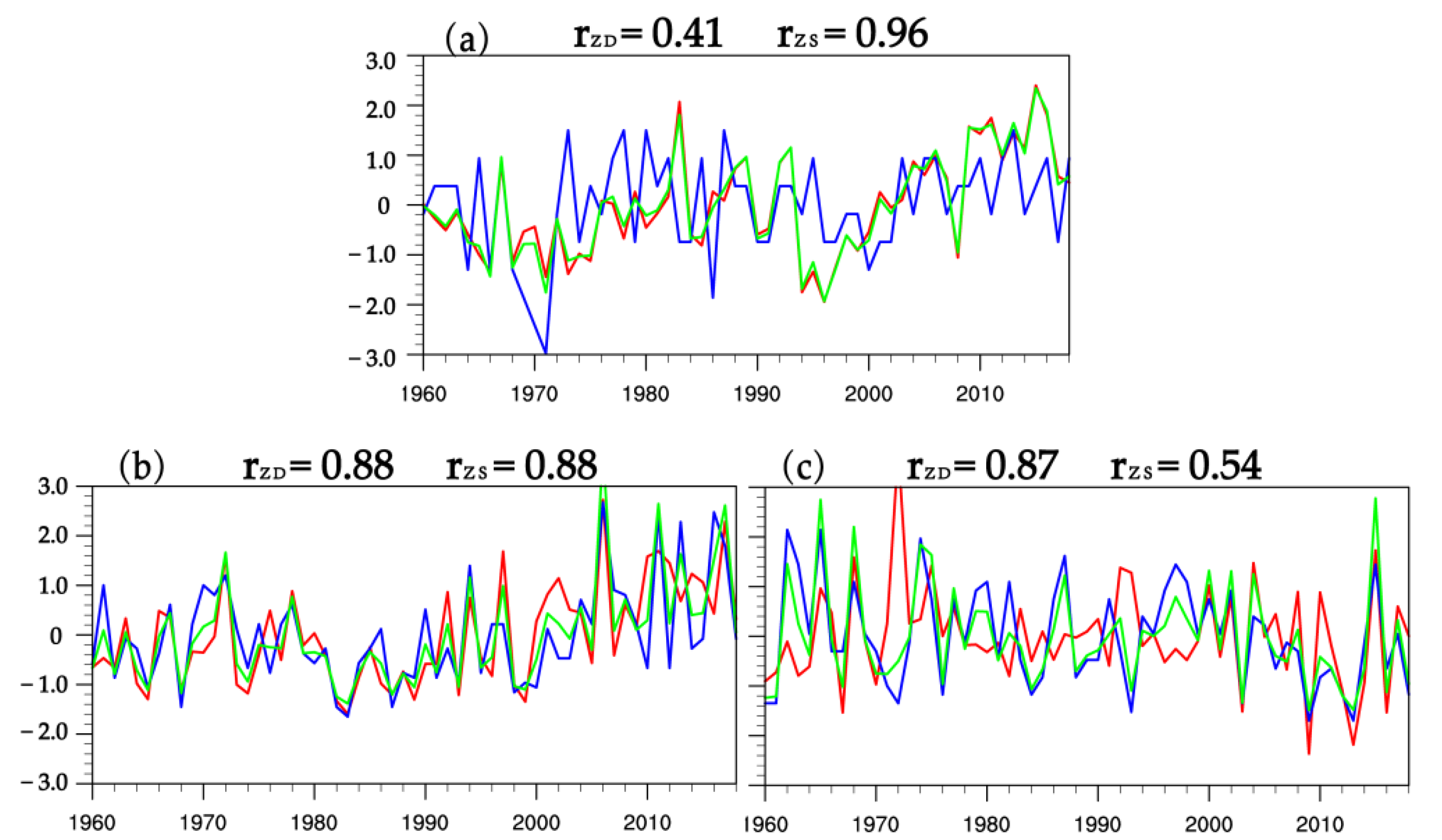
3.3. Regional Difference of the Response

In Figure 5, for each station, the variation rate of F-value caused by each 1 °C rise in the threshold is given and interpolated to form a spatial distribution map. Considering the nationwide, when the threshold is relatively high, there are a large number of missing stations in high latitudes and high altitudes areas, and the error in the spatial distribution after interpolation is pretty large. Therefore, only the temperature range of 27–33 °C is given in Figure 5.

The previous sections showed that the dominant results of summer accumulated temperature in different regions are sensitive to the change of threshold, that is, as the threshold increases, the dominant factor of stations in different regions change from intensity to number of days at different variation rates. Based on this difference, meaning the regional characteristics of the distribution of the variation rate, five more consistent regions of the rates were selected in the national station range, namely, region I, region II, region III, region IV, and region V (Figure 5).

The specific scope of each region is region I: 39−47° N, 121−132° E; region II: 34−39° N, 115−123° E; region III: 28−33° N, 116−123° E; region IV: 21−25° N, 105−114° E; region V: 27−34° N, 98−106° E.

At 27 °C, the calculation result of accumulated temperature in the Northeast region is positive, which means in this area, the dominant factor is the number of hotness days. Moreover, as threshold increases, the importance of days increases. While in other regions, the calculation result at 27 °C is negative, that is, the accumulated temperature is dominated by hotness intensity and gradually turns from intensity into days. Studies have confirmed that the rate of variation in all regions is positive, that is, as the threshold increases, the trend of the dominant factor changing from intensity to days is definite, but the magnitude of the slope varies, indicating that the transformation rates have differences. The greater the transformation rate of the region, the faster the impact of the number of hotness days increases, and the greater the temperature fluctuation amplitude in summer.

The stations average of the accumulated temperature dominance results for each region selected in Figure 5 is recorded as its regional dominance result, and its trend with increasing threshold is plotted in Figure 6. It can be seen that at 27 °C, the dominance results for all five regions are negative, i.e., at this threshold, the accumulated temperature in those regions are mainly influenced by intensity. As the threshold increases, the relative influence of the days increases. At a certain temperature when the threshold rises, the main influence factor turns into intensity from the number of days. The rate of change is positive in all regions, i.e., the trend of the main influence factor of the accumulated temperature in each region from intensity to days is consistent. The slope and trend are different, and the temperature point at which the curve changes from negative to positive is also different.

The distribution pattern of the variation rate of each region is basically decreasing from south to north. The high rate of regional transition, which means that the impact of the number of days increases more rapidly, indicates that the temperature variation in the region is relatively large. Once the threshold was raised, the number of days fluctuated dramatically. In the north-south direction, the transition rate is I < II < III < IV, that is, the closer the eastern region is to the tropics the greater the transition rate.

The temperature points of the main influence factor from days to intensity in each region are 28.5 °C in region I; 30.8 °C in region II; 32.3 °C in region III; 32.7 °C in region IV; and 29.6 °C in region V. In addition, the distribution pattern of these temperature points is basically consistent with the distribution of regional summer temperature conditions, so an attempt is made to use these points as the accumulated temperature threshold for the region and to develop related discussions.

Taking the southernmost region III (green curve) as an example, when 32.7 °C is its regional accumulated temperature threshold, it is able to represent the characteristics of both statistical feature factors of number of days and intensity in a more balanced way, and also to delineate the common and less common daily maximum temperatures, which is of some significance in operational forecasting and warning. When the threshold varies below 32.7 °C, the number of high temperature days changes little, which means that daily maximum summer temperatures above the threshold are common in the region. When the threshold varies above 32.7 °C, the number of days exceeding the threshold varies considerably, i.e., summer days exceeding the threshold are relatively uncommon in the region and are noteworthy in forecast operations. The same is true in other regions.

Therefore, we believe that the accumulated temperature under the regional threshold can be used as an index to reflect the summer hotness in certain regions. This threshold has the following advantages over the commonly used 35 °C: not only can it reflect the characteristics of the variation of both local days and intensity in a relatively balanced way, but also it is more flexible, as each region has its own specific regional threshold, which reduces the error caused by the climate difference between regions when studying the variation of accumulated temperature.

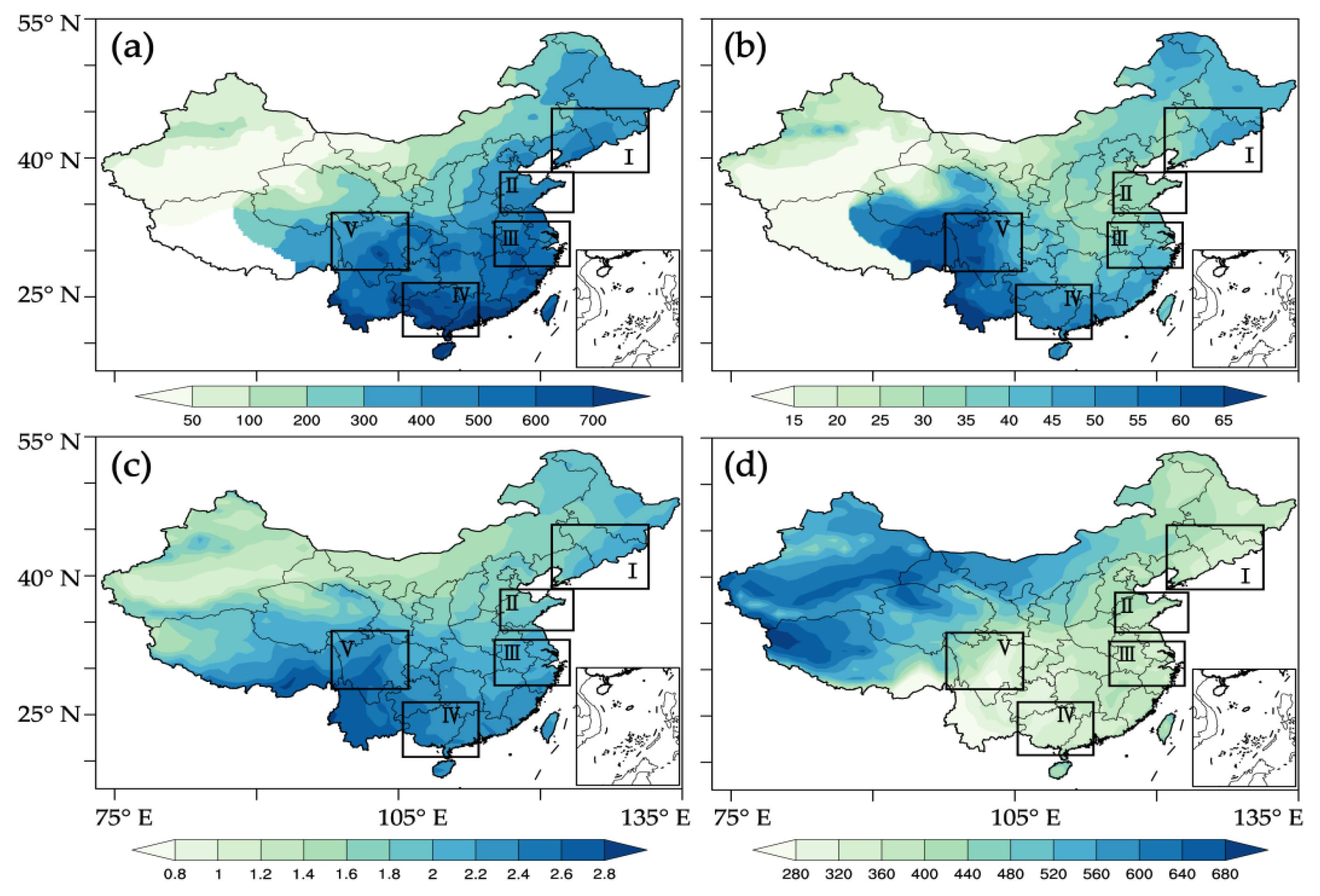
3.4. The Influencing Factors of Accumulated Temperature

In this section, in order to better understand the distribution and change trend of accumulated temperature, the relationship between accumulated temperature and precipitation, cloud cover, and solar radiation in various regions will be analyzed. An attempt will be made to explain the distribution pattern and change trend of cumulus temperature in terms of the correlation between accumulated temperature and others.

The partitions in Figure 7 are consistent with those in Figure 5, namely, regions I, II, III, IV, and V. In Figure 7a, the magnitude of total summer precipitation varies among regions, by size: IV > II > V > III > I. In Figure 7b, the magnitude of summer precipitation days varies among regions, by size: V > IV > I > III > II. In Figure 7c, the magnitude of summer total cloud cover varies among regions, by size: V > IV > I > III > II.

Using the data of accumulated temperature, precipitation and precipitation days in five regions from 1960 to 2018, and the data of accumulated temperature, total cloud cover and solar radiation from 1979 to 2018, the correlation between accumulated temperature and these elements is calculated (

Table 1. Correlation between regional accumulated temperature and influencing factors.

Region	TCC	DSRF	PRE	PD
I	−0.75 ***	0.75 ***	−0.40 **	−0.70 ***
II	−0.74 ***	0.70 ***	−0.16	−0.23
III	−0.63 ***	0.76 ***	−0.65 ***	−0.77 ***
IV	−0.47 **	0.49 ***	−0.55 ***	−0.54 ***
V	−0.77 ***	0.82 ***	−0.21	−0.50 ***

Notes: total cloud cover (TCC), direct shortwave radiation flue (DSRF), precipitation (PRE), and precipitation days (PD). **: significance level of 99%; ***: significance level of 99.9%.

).

The results showed that, among the five regions, their regional accumulated temperatures were negatively correlated with total cloudiness, precipitation, and precipitation days, and positively correlated with solar radiation.

The main influencing factors in region I are TCC and DSRF, both of which correlated with accumulated temperature up to 0.75. In addition, the correlation between PD and accumulated temperature also exceeded the 99.9% significance level. The main influencing factor in region II is TCC, while PRE and PD have less influence on the accumulated temperature. The main influencing factor in region III is PD. The main influencing factor in region IV is PRE. Furthermore, the factor in region V is DSRF with a correlation coefficient of 0.82, while the correlation of PRE is relatively low.

4. Conclusions and Discussion

4.1. Conclusions

The accumulated temperature is a comprehensive manifestation for both the number of hotness days and hotness intensity. Its variation is affected by both of frequency and intensity. In this study, we used the method of linear regression to explore the relative importance of the days and intensity in accumulated temperature. By selecting different temperatures as the threshold, the variation of the domination of accumulated temperature in thresholds and the regional characteristics of variation are studied in this research.

It is found that when a relative low threshold is used to define the “hotness day”, the accumulated temperature of most stations is dominated by hotness intensity. The dominant factor of accumulated temperature is sensitive to threshold. For a single station, as the threshold increases, the relative influence of intensity decreases, while the influence of the days increases gradually. For national stations, the number of stations which accumulated temperature dominated by hotness intensity decreases, while that dominated by hotness days increases. Compared with empirical theory, the change of domination is reasonable, and the use of linear regression method is also reliable.

4.2. Discussion

As mentioned above, there are other methods for analyzing the dominance. What we used here is a simple method. It needs to obtain a linearly-fitted relation, and the fitting needs to be statistically significant. Based on the linear relation, it is convenient to compare the relative importance of the different influencing variables. The method is actually similar to the error assessment in physics.

In the study, we selected five regions, given their own accumulated temperature thresholds. The regional accumulated temperatures with those thresholds have the reasonableness as a summer high temperature index. The reasons are as follows: firstly, the two statistical characteristic factors of accumulated temperature in each region, the number of days and intensity, have approximately the same effect on it. Secondly, when the temperature is below this regional threshold, the number of high temperature days varies little and the threshold temperature is a common summer temperature; when the temperature is above this regional threshold, the days start to decrease significantly; therefore, it can also be used as a temperature for regional weather temperature warning. Thirdly, the regional threshold pair is more flexible than the commonly used 35 °C, and each region has its own specific regional threshold, narrowing down the errors caused by regional differences in climate when using accumulated temperatures for statistical comparisons.

In future studies, we will attempt to select the temperature when the dominant result of accumulated temperature in each region is 0 as the high temperature threshold, compare the commonly used threshold of 35 °C [15,55,63,64,65], so as to study the judgment effect of accumulated temperature on summer high temperature under this threshold. It will further deepen the research on the rationality and applicability of accumulated temperature index and expand the application of research content in practice.

References

1. Qin, D.; Thomas, S. Highlights of the IPCC working group Ⅰ fifth assessment report. Clim. Chang. Res. 2014, 10, 1–6. [Google Scholar]
2. Matuszko, D.; Weglarczyk, S. Relationship between sunshine duration and air temperature and contemporary global warming. Int. J. Climatol. A J. R. Meteorol. Soc. 2015, 35, 3640–3653. [Google Scholar]
3. Zhou, B.; Qian, J. Changes of weather and climate extremes in the IPCC sixth assessment report. Clim. Chang. Res. 2021, 17, 713–718. [Google Scholar]
4. Karl, T.R.; Easterling, D.R. Climate extremes: Selected review and future research direction. Clim. Chang. 1999, 42, 309–325. [Google Scholar] [CrossRef]
5. Alexander, L.V.; Zhang, X.; Peterson, T.C.; Caesar, J.; Gleason, B.; Tank, A.M.G.K.; Haylock, M.; Collins, D.; Trewin, B.; Rahimzadeh, F. Global observed changes in daily climate extremes of temperature and precipitation. J. Geophys. Res. Atmos. 2006, 111, D05109. [Google Scholar] [CrossRef] [Green Version]
6. Ding, Y. National assessment report of climate change(I): Climate change in China and its future trend. Clim. Chang. Res. 2006, 2, 3–8. [Google Scholar]
7. Zhai, P.; Pan, X. Change in extreme temperature and precipitation over northern China during the second half of the 20th century. Acta Geogr. Sin. 2003, 58, 1–10. [Google Scholar]
8. Tan, J.; Zheng, Y.; Peng, L. Effect of urban heat island on heat waves in summer of Shanghai. Plateau Meteorol. 2008, 27, 144–149. [Google Scholar]
9. Zhang, Y.; Cao, L.; Xu, Y. Scenario analyses on future changes of extreme temperature events over China. J. Appl. Meteorol. Sci. 2008, 19, 655–660. [Google Scholar]
10. Ren, G.; Feng, G.; Yan, Z. Progresses in observation studies of climate extremes and changes in mainland China. Clim. Environ. Res. 2010, 15, 337–353. [Google Scholar]
11. Wu, R.; Zheng, Y.; Liu, J. Trand analysis of high temperature disaster in large cities of the Yangtze River Delta. J. Nat. Disasters 2010, 19, 56–63. [Google Scholar]
12. Xiao, S.; Zhang, K.; Liu, F. Study of high-temperature and heatwaves in Shijiazhuang compared to the “three-furnace cities” in China. Geogr. Geo-Inf. Sci. 2010, 26, 87–92. [Google Scholar]
13. Zhang, X.; Ning, H.; Du, J. The impact of urban heat island effect on high temperature in summer in Xi’an. J. Arid. Land Resour. Environ. 2010, 24, 95–101. [Google Scholar]
14. Zhang, K.; Li, Z.; Liu, J. Temporal-spatial feature analysis on the high-temperature and heatwaves in Hebei and its influence on industry and transportation. Geogr. Geo-Inf. Sci. 2011, 27, 90–95. [Google Scholar]
15. Chen, M.; Geng, F.; Ma, L.M.; Zhou, W.D.; Shi, H.; Ma, J.H. Analyses on the heat wave events in Shanghai in recent 138 Years. Plateau Meteorol. 2013, 32, 2597–2607. [Google Scholar]
16. Li, Y.; Li, H.; Ye, P.; Zhu, C. Analysis of extreme high temperature events in summer during 1980–2010 over north China. J. Lanzhou Univ. 2014, 50, 832–837. [Google Scholar]
17. Zhou, B.; Xu, Y.; Wu, J.; Dong, S.; Shi, Y. Changes in temperature and precipitation extreme indices over China: Analysis of a high-resolution grid dataset. Int. J. Climatol. 2015, 36, 1015–1066. [Google Scholar] [CrossRef]
18. Jiang, R.; Chen, L.; Xiang, W. Characteristics of extreme high temperature weather in Shanghai. J. Meteorol. Environ. 2016, 32, 66–74. [Google Scholar]
19. Zhang, X.; Li, X. Spatial-temporal characteristics and causes of summer heat waves in Hunan province. Clim. Environ. Res. 2017, 22, 747–756. [Google Scholar]
20. Wu, J.; Zhu, H.; Zong, P.; Hui, P.; Tang, J. Analysis on the spatial-temporal features of temperature extremes in the Yangtze-huaihe river basin over the past decades: Comparison between observation and reanalysis. J. Meteorol. Sci. 2018, 38, 464–476. [Google Scholar]
21. He, L.; Jian, M. Temporal variations of extreme heat days in Guigang of Guangxi and related circulation background. J. Trop. Meteorol. 2019, 35, 694–708. [Google Scholar]
22. Jiang, X.; Jiang, Z.; Li, W. Risk estimation of extreme high temperature in eastern China under 1.5 and 2 °C global warming. Trans. Atmos. Sci. 2020, 43, 1056–1064. [Google Scholar]
23. Wang, Y.; Ma, H.; Li, H. Responses of summer high temperature of urban agglomeration in Yangtze River Delta to global warming in the future. J. Meteorol. Sci. 2021, 41, 285–294. [Google Scholar]
24. Li, Z.; Li, C.; Song, J.; Tan, Y.; Li, X. An analysis of characteristics and causes of extremely high temperature days in the Yangtze-Huaihe river basins in summer 1960–2011. Clim. Environ. Res. 2015, 20, 511–522. [Google Scholar]
25. Liu, L. Global extreme weather normalization. Ecol. Econ. 2021, 37, 5–8. [Google Scholar]
26. Poumadere, M.; Mays, C.; Le Mer, S.; Blong, R. The 2003 heat wave in France: Dangerous climate change here and now. Risk Anal. 2005, 25, 1483–1494. [Google Scholar] [CrossRef]
27. Martiello, M.A.; Giacchi, M.V. High temperatures and health outcomes: A review of the literature. Scand. J. Public Health 2010, 38, 826–837. [Google Scholar] [CrossRef]
28. Yang, H.; Chen, Z.; Xie, S. Quantitative assessment of impact of extreme high temperature in summer on excess mortality in Wuhan. J. Meteorol. Environ. 2013, 29, 140–143. [Google Scholar]
29. Liu, H.; He, L.; Yang, Q. Spatial inequality and distributional dynamics of population ageing in China, 1989–2011. Popul. Res. 2014, 38, 71–82. [Google Scholar]
30. Li, T.; Du, Y.; Mo, Y.; Du, Z.; Huang, L.; Cheng, Y. Human health risk assessment of heat wave based on vulnerability: A review of recent studies. J. Environ. Health 2014, 31, 547–550. [Google Scholar]
31. Xia, J.J.; Tu, K.; Yan, Z.; Qi, Y. The super-heat wave in eastern China during July–August 2013: A perspective of climate change. Int. J. Climatol. 2016, 36, 1291–1298. [Google Scholar] [CrossRef]
32. Schlegel, I.; Muthers, S.; Mücke, H.-G.; Matzarakis, A. Comparison of respiratory and ischemic heart mortalities and their relationship to the thermal environment. Atmosphere 2020, 11, 826. [Google Scholar] [CrossRef]
33. Diniz, F.R.; Gonçalves, F.L.T.; Sheridan, S. Heat wave and elderly mortality: Historical analysis and future projection for metropolitan region of São Paulo, Brazil. Atmosphere 2020, 11, 933. [Google Scholar] [CrossRef]
34. Grigorieva, E.; Lukyanets, A. Combined effect of hot weather and outdoor air pollution on respiratory health: Literature review. Atmosphere 2021, 12, 790. [Google Scholar] [CrossRef]
35. Žiberna, I.; Pipenbaher, N.; Donša, D.; Škornik, S.; Kaligarič, M.; Bogataj, L.K.; Črepinšek, Z.; Grujić, V.J.; Ivajnšič, D. The impact of climate change on urban thermal environment dynamics. Atmosphere 2021, 12, 1159. [Google Scholar] [CrossRef]
36. Grigorieva, E.A.; Revich, B.A. Health risks to the Russian population from temperature extremes at the beginning of the XXI century. Atmosphere 2021, 12, 1331. [Google Scholar] [CrossRef]
37. Shevchenko, O.; Snizhko, S.; Zapototskyi, S.; Matzarakis, A. Biometeorological conditions during the August 2015 mega-heat wave and the summer 2010 mega-heat wave in Ukraine. Atmosphere 2022, 13, 99. [Google Scholar] [CrossRef]
38. Graczyk, D.; Pińskwar, I.; Choryński, A. Heat-related mortality in two regions of Poland: Focus on urban and rural areas during the most severe and long-lasting heatwaves. Atmosphere 2022, 13, 390. [Google Scholar] [CrossRef]
39. Huang, X.; Wang, B.; Liu, M.; Guo, Y.; Li, Y. Characteristics of urban extreme heat and assessment of social vulnerability in China. Geogr. Res. 2020, 39, 1534–1547. [Google Scholar]
40. Dai, P.; Li, H.; Luo, H.X.; Zhao, Y.F. The spatio-temporal change of active accumulated temperature ≥10 °C in southern China from 1960 to 2011. Acta Geogr. Sin. 2014, 69, 650–660. [Google Scholar]
41. Real, A.C.; Borges, J.; Cabral, J.S.; Jones, G.V. A climatology of vintage port quality. Int. J. Climatol. A J. R. Meteorol. Soc. 2017, 37, 3798–3809. [Google Scholar] [CrossRef]
42. Xie, B.; Guo, L.; Du, D.; Tan, Y.; Wang, G. Responses of camellia oleifera yield to heat accumulation temperature and high temperature days in key growth period. Sci. Silvae Sin. 2021, 57, 34–42. [Google Scholar]
43. Liu, D.; Dong, A.; Deng, Z. Impact of climate warming on agriculture in northwest China. J. Nat. Resour. 2005, 20, 119–125. [Google Scholar]
44. Ma, J.; Liu, Y.; Yang, X.; Wang, W.F.; Xue, C.Y.; Zhang, X.Y. Characteristics of climate resources under global climate change in the north China plain. Acta Ecol. Sin. 2010, 30, 3818–3827. [Google Scholar]
45. Yuan, S.; Gu, X.; Xiang, H.; Wang, F.; Kang, W.; Yu, F. Distribution of accumulated temperature of high spatial resolution over complex terrains across the Guizhou plateau based on GIS. Resour. Sci. 2010, 32, 2427–2432. [Google Scholar]
46. Li, S.; Shen, Y. Impact of climate warming on temperature and heat resource in arid northwest China. Chin. J. Eco-Agric. 2013, 21, 227–235. [Google Scholar] [CrossRef]
47. Li, C.; Yang, P.; Liu, W.; Li, D.Y.; Wang, Y. An analysis of accumulative effect of temperature in short-term load forecasting. Autom. Electr. Power Syst. 2009, 33, 96–99. [Google Scholar]
48. Xiao, W.; Luo, D.; Dong, X. Analysis of accumulated temperature effect and application in forecasting. Microcomput. Inf. 2009, 25, 262–264. [Google Scholar]
49. Fang, G.; Hu, C.; Zheng, Y.H.; Cai, J.M. Study on the method of short-term load forecasting considering summer weather factors. Power Syst. Prot. Control 2010, 38, 100–104. [Google Scholar]
50. Gao, W.; Li, Q.; Su, W.; Li, Y. Temperature correction model research considering temperature cumulative effect in short-term load forecasting. Trans. China Electrotech. Soc. 2015, 30, 242–248. [Google Scholar]
51. Xie, X.; Li, Y.; Hang, X.; Huang, S. The effect of air temperature on the process of cyanobacteria recruitment and dormancy in Lake Taihu. J. Lake Sci. 2016, 28, 818–824. [Google Scholar]
52. Sun, X.; Zhu, G.; Da, W.; Yu, M.L.; Yang, W.B.; Zhu, M.Y.; Xu, H.; Guo, C.X.; Yu, L. Effects of hydrological and meteorological conditions on diatom proliferation in reservoirs. Environ. Sci. 2018, 39, 1129–1140. [Google Scholar]
53. Li, D.; Li, L.; He, Y.; Gou, S.; Zhao, N. Characteristics of vegetation growth period and its response to climate change in Zoigê Area from 2001 to 2015 based on remote sensing data. Adv. Eng. Sci. 2019, 51, 165–172. [Google Scholar]
54. Zhou, Q.; Bian, J.; Zheng, J. Variation of air temperature and thermal resources in the northern and southern regions of the Qinling mountains from 1951 to 2009. Acta Geogr. Sin. 2011, 66, 1211–1218. [Google Scholar]
55. Miu, Q.; Pan, W.; Xu, X. Characteristic analysis of summer temperature in Nanjing during 56 years. J. Trop. Meteorol. 2008, 24, 737–742. [Google Scholar]
56. Azen, R.; Budescu, D.V. The dominance analysis approach for comparing predictors in multiple regression. Psychol. Methods 2003, 8, 129–148. [Google Scholar] [CrossRef]
57. Budescu, D.V.; Azen, R. Beyond global measures of relative importance: Some insights from dominance analysis. Organ. Res. Methods 2004, 7, 341–350. [Google Scholar] [CrossRef]
58. Behson, S.J. The relative contribution of formal and informal organizational work–family support. J. Vocat. Behav. 2005, 66, 487–500. [Google Scholar] [CrossRef]
59. Lu, E.; Zeng, Y.; Luo, Y.; Ding, Y.; Zhao, W.; Liu, S.; Gong, L.; Jiang, Y.; Jiang, Z.; Chen, H. Changes of summer precipitation in China: The dominance of frequency and intensity and Linkage with changes in moisture and air temperature. J. Geophys. Res. 2015, 119, 12575–12587. [Google Scholar] [CrossRef]
60. Lu, E.; Ding, Y.; Zhou, B.; Zou, X.; Chen, X.; Cai, W.; Zhang, Q.; Chen, H. Is the interannual variability of summer rainfall in China dominated by precipitation frequency or intensity? An analysis of relative importance. Clim. Dyn. 2016, 47, 67–77. [Google Scholar] [CrossRef]
61. Lu, E.; Tu, J. Relative importance of surface air temperature and density to interannual variation in monthly surface atmospheric pressure. Int. J. Climatol. 2021, 41, E819–E831. [Google Scholar] [CrossRef]
62. Hua, W.; Chen, H. Response of land surface processes to global warming and its possible mechanism based on CMIP3 multi-model ensembles. Atmos. Sci. 2011, 35, 121–133. [Google Scholar]
63. Zhang, T.; Cheng, B. Variation and scenario projections of heat wave duration index and warm night index in Chongqing. Meteorol. Sci. Technol. 2010, 38, 695–703. [Google Scholar] [CrossRef]
64. Xiao, A.; Zhou, C. Characteristic analysis of the heat wave events over China based on excess heat factor. Meteorol. Mon. 2017, 43, 943–952. [Google Scholar]
65. Yang, H.; Ma, Y.; Shi, J. Spatial and temporal characteristics of summertime high temperature in Yangtze River delta under the background of global warming. Resour. Environ. Yangtze Basin 2018, 27, 1544–1553. [Google Scholar]
Figure 1. (a) Scatter diagram at 27 °C. a is the coefficient of days, b is the coefficient of intensity. (b) Spatial distribution map of 27 °C: b > 2a: dark blue; 2a > b > a: light blue; a > 2b: dark red; 2b > a > b: light red.
Atmosphere 13 00819 g001
Figure 2. Red line: intensity; blue line: days; green line: accumulated temperature. rZD: correlation coefficient between accumulated temperature and days, rZS: correlation coefficient between accumulated temperature and intensity.
Atmosphere 13 00819 g002
Figure 3. (a) Scatter plot at 28 °C, the black line is coefficient a = b; (b) spatial distribution map at 28 °C; (c) scatter plot at 32 °C; (d) spatial distribution map at 32 °C; (e) scatter plot at 36 °C; (f) spatial distribution map at 36 °C.
Atmosphere 13 00819 g003
Figure 4. Red line: intensity; blue line: days; green line: accumulated temperature. rZD: correlation coefficient between accumulated temperature and days, rZS: correlation coefficient between accumulated temperature and intensity. Interannual variation graph: (a) 28 °C, (b) 32 °C, (c) 36 °C.
Atmosphere 13 00819 g004
Figure 5. Distribution of change rate of dominant results with the increase of threshold. (a) 27−28 °C, (b) 28−29 °C, (c) 29−30 °C, (d) 30−31 °C, (e) 31−32 °C, (f) 32−33 °C. Boxes denote five regions.
Atmosphere 13 00819 g005
Figure 6. Dominance results of the five regions change with the threshold. The numbers in the legend are the average transition rates of each region. The green line is the area with the largest transition rate, the blue line is the area with the smallest transition rate.
Atmosphere 13 00819 g006
Figure 7. Spatial distribution of summer in China. (a) Precipitation (mm), (b) the number of precipitation days (days), (c) total cloud cover (%), (d) direct shortwave radiation flue (W·m−2).
Atmosphere 13 00819 g007