Article

Investigation of Policy Relevant Background (PRB) Ozone in East Asia

1
Department of Geography, University of Hong Kong, Hong Kong, China
2
School of Energy and Environment, City University of Hong Kong, Hong Kong, China
3
School of Earth and Environmental Sciences, Seoul National University, Seoul 08826, Korea
*
Author to whom correspondence should be addressed.
Atmosphere 2022, 13(5), 723; https://doi.org/10.3390/atmos13050723
Submission received: 4 April 2022 / Revised: 27 April 2022 / Accepted: 28 April 2022 / Published: 1 May 2022
(This article belongs to the Special Issue Air Pollution and Climate Issues in the Coastal Atmosphere of China)

Abstract

:
The concept of Policy Relevant Background (PRB) ozone has emerged in recent years to address the air quality baseline on the theoretical limits of air pollution controls. In this study, the influence of Long-range Transport (LRT) of air pollutants from North America and the effect of Stratosphere-Troposphere Transport (STT) on PRB ozone was investigated using GEOS-Chem coupled WRF-CMAQ modelling system. Four distinct seasons in 2006 were simulated to understand better the seasonal and geographical impacts of these externalities on PRB ozone over East Asia (EA). Overall, the LRT impact from North America has been found to be ~0.54 ppbv, while the maximum impacts were found at the mountain stations with values of 2.3 ppbv, 3.3 ppbv, 2.3 ppbv, and 3.0 ppbv for January, April, July, and October, respectively. In terms of PRB ozone, the effect of STT has enhanced the surface background ozone by ~3.0 ppbv, with a maximum impact of 7.8 ppbv found in the northeastern part of East Asia (near Korea and Japan). Springtime (i.e., April) has the most vital STT signals caused by relatively cold weather and unstable atmospheric condition resulting from the transition of the monsoon season. The simulated PRB ozone based on the mean values of the maximum daily 8-h average (MDA8) is 53 ppbv for spring (April) and 22 ppbv for summer (July). Up to ~1.0 ppbv and ~2.2 ppbv of MDA8 ozone were attributed to LRT and STT, respectively. Among the selected cities, Beijing and Guangzhou have received the most substantial anthropogenic enhancement in MDA8 ozone in summer, ranging from 40.0 ppbv to 56.0 ppbv.

1. Introduction

The chemical composition of the atmosphere has significantly changed during the last few decades due to anthropogenic influences. Photochemical smog (a by-product of industrialization), partially contributed by ozone air pollution, has become a serious health-related problem in urban environments [1]. Ozone air pollution has received continuous attention from local and regional governments in East Asia.
The term, Policy Relevant Background (PRB) ozone (the term first appeared in North America) has emerged in recent years, which defines the background ozone level in the absence of local anthropogenic emissions via the air quality/chemical transport models [2]. The purpose of PRB is to estimate the maximum achievable ozone reduction through anthropogenic emission controls. It is an important baseline value for which policymakers are used to address some local areas where ozone pollution is dominated by non-local and non-anthropogenic sources [3]. It has been observed that the PRB is somewhat like the background ozone defined by the measurement community, where observation is taken from the relatively remote monitoring sites with minimal influence from local anthropogenic emissions to understand local background ozone. Li et al. [4] and Ou Yang et al. [5] reported that the monthly ozone in their stations ranges from 22 to 73 ppbv, with the highest value observed at Mt. Tai (1534 m a.s.l.) during springtime. This reported range is similar to the value of 25–60 ppbv observed over North America [6]. As these stations are located at highly elevated mountains above the planetary boundary layer, the effects of long-range transport of air pollutants from different continents and stratosphere-troposphere transport were also captured. In a US air quality study, Hogrefe et al. [7] reported that the contributions of these non-local (i.e., long-range transport) and natural (i.e., stratosphere-troposphere transport) sources could account for up to 46% of the overall ozone [2,8], which illustrates the importance of these phenomena in defining local air quality and PRB ozone.
Observation-based research, which utilized remote sensing techniques (i.e., MODIS satellite images), has confirmed the presence of intercontinental transport of air pollutants via large wildfire or dust storm events [9,10,11]. The pollution enhancement from Long-Range Transport (LRT) not only alters the photochemical condition in the free troposphere but also affects the background concentrations of different chemical constituents at the ground level, influencing both local and regional air quality. Various studies have confirmed that peroxyacetyl nitrate (PAN) formed from NOx and/or non-methane volatile organic compounds (NMVOCs) is one of the major contributors to the enhancement of surface ozone in LRT events [12,13,14]. The enhancement mechanism involves the formation and transport of PAN at the free troposphere and the thermal decomposition of NOx during subsidence at the receptor region. The magnitude of LRT is strongly influenced by: (1) the relative difference between self-emission situation and the number of pollutants being transported; (2) the distance between source and receptor, and regional meteorology (e.g., seasonal influence) [3]. Generally, the impact of LRT on the surface is more noticeable in later winter and early spring at highly elevated locations but less pronounced in summer and at the ground level [15]. From the geographical perspective, it has been reported that the air quality impact of LRT over North America (NA) from East Asia (EA) outflows is much stronger than the impacts caused by NA outflows over EA, as the anthropogenic emission strength at EA is much stronger than at NA. Moreover, with the effective outflow mechanism through westerlies, the emission enhancement from EA has resulted in about 9.0 ± 3 ppbv of ozone increases over NA [4,8]. In EA, Fu et al. [16] reported that the LRT of air pollutants from other continents has also contributed to ozone enhancement over EA, which intensified the monthly surface ozone by 0.1–0.23 ppbv. They reported that the strongest LRT influence over EA comes from NA outflows, followed by South Asia and Europe outflows. Lee et al. [17] reported that Africa and Southeast Asia also contributed to pollution enhancement over EA during the biomass burning seasons.
Another important source of surface ozone enhancement is Stratosphere-Troposphere Transport (STT), which is one of the significant contributors to the tropospheric ozone budget [18,19]. Lin et al. [20] reported that rapid stratospheric-tropospheric intrusion could increase surface ozone up to 25 ppbv at the highly elevated sites (e.g., 2–3 km above the mean sea level) in the western United States. Strong location dependence (i.e., latitude and altitude) and noticeable seasonal variation of STT influence on tropospheric ozone were also reported in other studies [19,21]. It should be aware that the STT values reported in the literature may be subjected to high uncertainty due to the uncertainty of defining tropopause and near-tropopause ozone and inter-model differences in tropospheric chemistry and physics [19]. Nevertheless, these STT values still provide essential information for understanding stratosphere-troposphere interactions. In regional air quality modeling, STT is incorporated through the lateral boundary conditions (i.e., top and side boundaries) using global or hemispheric chemical transport models (e.g., GEOS-Chem, MOSAIC, or CCSM). Various simulation approaches (e.g., chemical downscaling and observational reanalysis) have been developed to describe better the chemical boundaries under the limited domain environment [6,21,22]. Currently, regional STT studies that focus on the impact of surface ozone are concentrated in North America, possibly due to the increasing importance of STT ozone on the overall ozone budget in the last decade and the richness of available data from various networks (e.g., CASTNET, WOUDC, etc.) [3,7]. To our best knowledge, no regional modelling study has assessed the STT influence over East Asia in the context of PRB ozone.
In this study, the GEOS-Chem global chemical transport model coupled with the WRF-CMAQ air quality modelling system was used to quantify the effects of LRT and STT on PRB ozone over EA. Multi-boundary cases from GEOS-Chem with different CMAQ emission scenarios were adopted to study self-emission, LRT, and STT impacts, aiming to define the regulatory PRB ozone in EA. The PRB ozone assessment was carried out over the selected cities and different climatic zones to reflect better the importance of geographical differences in ozone prediction. The focus of the study was placed on better understanding the seasonal influence and spatial variation of STT in the context of PRB ozone. To our best knowledge, this is the first study investigating both LRT and STT influences on regional ozone in EA. The paper is organized as follows. Section 2 covers the methodology and air quality models used in the study. Section 3.2 discusses the impact of long-range transport, and Section 3.3.2 elaborates on the influence of stratospheric ozone on PRB ozone. Finally, Section 3.3.3 summarizes the maximum daily 8-h average ozone for the selected Asian cities and regions.

2. Materials and Methods

2.1. Study Area and Scope of the Study

The WRF-CMAQ-based PATH modelling system was adopted to study the effects of LRT, STT, and PRB ozone over EA. The PATH system is the model used by Hong Kong Environmental Protection Department (HKEPA) for studying Pollutants in the atmosphere and their Transport over Hong Kong. The system has been validated intensively via in-house and contracted studies [23]. The PATH platform comprises four nested domains from 27 km Asia and Southeast Asia (D1) down to 1 km Hong Kong (D4). For this study, only D1, which covers multiple countries, including China, Japan, North Korea, South Korea, Myanmar, Laos, Northern Thailand, and Vietnam, was applied, as shown in Figure 1. A detailed description of the PATH system is discussed in Section 2.3. The target periods of this study are January, April, July, and October of 2006. To achieve the study objectives, multiple GEOS-Chem boundary cases with different emission removals were implemented to generate CMAQ boundary conditions. For evaluating seasonal and geospatial variations of PRB ozone, climatic zones (as shown in Figure 1) were adopted to represent the ozone changes over EA. Moreover, multiple megacities/cities were selected for comparative ozone assessment, including Hong Kong, Guangzhou, Shanghai, Beijing, Chongqing, Tianjin, Seoul, Tokyo, and Taipei. Details of each component are summarized below.

2.2. GEOS-Chem Boundary Condition for Long-Range Transport Influence

The GEOS-Chem model version 8-02-03 for ozone-PM-Hg was applied to produce the boundary conditions for 2006 CMAQ simulations [24]. This version of GEOS-Chem came with a number of updates, including bromine chemistry and updated emissions and scavenging [25]. The simulation was conducted at a resolution of 2° × 2.5° horizontal resolution with 3-h temporal resolution on 47 vertical layers simulated by GEOS-5 meteorological input. To investigate emission influence over EA, three simulation cases were established, which are (1) Full EM: the actual emission case without any emission reduction; (2) Zero-out EA: sensitivity case with EA emission removal, and (3) Zero-out NA: sensitivity case with NA emission removal. Table 1 shows the summary of the cases with corresponding emission descriptions. The EA and NA emissions came from Streets, National Emissions Inventory (NEI05), Criteria Air Contaminants inventory (CAC), and BRAVO Emissions inventory. Simulations were performed for 2006 with four extra months from 2005 for the spin-off period.
To achieve emissions removal from GEOS-Chem, code modification in the current version of GEOS-Chem was performed. Different regional masks were applied to different sensitivity cases to achieve zero anthropogenic emissions (See Supplementary Materials Figure S1 for the masked areas used for the sensitivity study). The GEOS-Chem outputs from these cases were chemically downscaled to provide the LRT and STT signals via lateral boundary conditions for the regional CMAQ model. It intends to identify the ozone air quality impacts over EA using a fine-resolution model. Detailed downscaling methodology for obtaining boundary conditions and GEOS-Chem performance can be found in Lam and Fu [22] and Lam et al. [27].

2.3. WRF-CMAQ Air Quality Model

The WRF-CMAQ is a comprehensive atmospheric chemistry and transport model that numerically handles both physical and chemical processes, driven by the Weather Research Forecasting (WRF) model. The processes in CMAQ include subgrid turbulent vertical transport, horizontal and vertical advection, horizontal diffusion, cloud processes (i.e., aqueous chemistry, subgrid convective transport, wet deposition), gas-phase chemistry, and aerosol chemistry and dynamics. In this study, the WRF-CMAQ-based PATH modelling system was adopted. Details of WRF model setups, CMAQ air quality prediction, and WRF meteorology performance can be found in Environ [23]. For CMAQ emissions, the Intercontinental Chemical Transport Experiment-Phase B (INTEX-B) emissions supplemented with the Chinese Electricity Statistical Yearbook 2006, TRACE-P ship emission, and biomass burning were applied, which has been validated in various studies [26,28,29,30]. For natural emissions, MEGAN biogenic and sea-salt emissions were included. The multi-case inputs from GEOS-Chem output were downscaled to perform CMAQ simulation to provide initial and boundary conditions for the runs. The CMAQ model setups and scenarios used in this study are shown in Table 2 and Table 3, respectively. The first scenario is the base case where no emission adjustment has been made on both GEOS-Chem and CMAQ. The second scenario is called NA0, where North American anthropogenic emissions were removed from GEOS-Chem but no change to CMAQ emissions over EA. It is used to study the effect of LRT from NA over EA. The third and fourth scenarios are named EA0 and STT, respectively. In these scenarios, East Asian anthropogenic emissions from GEOS-Chem were removed from global emissions along with the removal of CMAQ EA anthropogenic emissions, which provides us with information on PRB ozone.
For the fourth scenario, the tropopause searching algorithm described in Lam and Fu [22] was adopted to remove the effect of stratospheric ozone from the upper level of the GEOS-Chem boundary condition to evaluate the influence of STT on PRB ozone. All emission scenarios were simulated at 27-km resolution, as mentioned earlier. The simulation periods cover (1) January (JAN): from 21 December 2005 to 31 January 2006, (2) April (APR): from 20 March 2006 to 30 April 2006, (3) July (JUL): from 20 June 2006 to 31 July 2006, and (4) October (OCT): from 20 September 2006 to 31 October 2006. These four months represent the four seasons in EA. For each simulation month, extra ten days were included as spin-off days for chemical initialization. Analysis was only performed on the actual months. Validation of CMAQ simulation for the full EMA case using observation data from Pearl River Delta can be found in Lam et al. [32].

3. Results and Discussion

3.1. Base Case Simulation

The base case simulation (i.e., Full EM emission condition) adopted from the PATH modelling system has been validated rigorously under the 1 km resolution during the development. Details of the model performance on local air quality prediction can be found in Environ [23]. As this study applied 27 km resolution simulation, pair comparisons of observation and model output were once revisited and evaluated. Figure 2a–d shows the hourly time series of two selected background stations for January and April. The remaining seasons (i.e., July and October), as well as the vertical ozone profile (for qualitative analysis), are also available in Figure S2. These background stations are Ryori, Japan (39°02′ N 141°49′ E at 260 m msl height) and Tap Mun, Hong Kong SAR (22°28′ N 114°21′ E at 26 m msl height), which are two of a few that were publicly available (i.e., 2006 data) from EA for the study period. These stations were used to evaluate the predictability of ozone from the 27 km simulations.
The top panel corresponds to Ryori station and the bottom panel is for Tap Mun station.
As shown in Figure 2 and Figure S2, the simulated ozone trends were, in general, consistent with the observation trends, with some overestimation found in January and April (Figure 2c,d) at Tap Mun station. A similar conclusion (Figure S2c) can also be drawn using the ozonesonde data (only four vertical profiles per month) obtained from King’s Park, Hong Kong (22°19′ N 114°10′ E). In general, the simulated mean values of vertical ozone (i.e., 30 or 31 profiles per month) were slightly higher than the observed values in January and April at the low and mid-troposphere. At the ground level, as shown in Table 4, the seasonal (monthly) mean differences of ozone ranged from −0.6 to −3.8 ppbv and −1.8 to 20.4 ppbv at Royoi and Tap mun, respectively, while the Root Mean Square Error (RMSE) from the hourly data ranged from 5.8 to 15.2 ppbv, and 17.9 to 33.3 ppbv. Overall, relatively larger RMSE were found in January and April (Figure 2c,d) at Tap Mun, possibly due to the overestimation of anthropogenic emissions in Southern China [26,33,34]. As extra emissions were transported to Hong Kong through northeasterly wind, it caused enhancements of ground-level ozone in the model. It should be noted that this study focused on the assessment of PRB ozone, which is irrelevant to the change in East Asia anthropogenic emissions. For the LRT investigation, the relative differences between cases would largely cancel out since the process involves subtracting two different simulations. Hence, the influence would be limited.

3.2. Seasonal Influence on Long-Range Transport over EA

To evaluate the effect of LRT over EA, the difference between the base case and NA0 from the hourly CMAQ simulations was used to reflect the emission contribution from NA. As ozone responds nonlinearly to the change of emission source, the difference between the base case and NA0 could be negative. Figure 3 shows the ozone enhancement of long-range transport from North America over East Asia using the Interquartile Range (IQR). The two edges of the box signify the 25% tiles from the median (e.g., center line). The cross sign (“x”) represents the mean value of the dataset, and the flat bars on the two far ends indicate the 1.5 IQR. Any data beyond the flat bars was considered an outlier.
In January, the mean ozone enhancement was 0.62 ppbv, with of IQR of 0.66 ppbv. In April, both the mean value (0.81 ppbv) and IQR (0.97 ppbv) increased. The range of ozone enhancement was also much more significant than that in January. A clear difference in ozone enhancement, however, is found in July. The mean value dropped to 0.21 ppbv, and the IQR shortened to 0.22 ppbv. The box also occupies a lower position than those two months. Although the IQR for July was very small, many data points belonged to outliers. The ozone enhancement rose again from July to October, in terms of mean (0.53 ppbv) and IQR (0.60 ppbv). Overall, the average LRT impact from NA over the four months was about 0.54 ppbv, comparable with the 0.23 ppbv reported by Fu et al. [16]. The maximum LRT impacts, indicated by the most extreme values from NA, were 2.27 ppbv, 3.25 ppbv, 2.28 ppbv, and 2.99 ppbv for January, April, July, and October, respectively. These values were mainly found at the elevated mountainous grids (i.e., Himalayas), which were at the level of the free troposphere. In terms of seasonal ozone impact, it is clear that April has received more impact than the other months, while July was the least affected.
Grouping the ozone enhancement data under different climatic zones (see Table 5), nearly all zones had their highest mean ozone values in April, except for the North Tropical zone (January), which is located at the south tip of China (i.e., Hainan Island, see Figure 1). Moreover, the lowest mean value for all climatic zones is found in July (except for the North Tropical zone, which had its lowest value found in October). These two remarks are consistent with the findings in Figure 3. Among the eight climatic zones, South Temperate and Mid-Temperate zones received much higher LRT impacts than the others, possibly due to their locations being direct downwind of the mid-latitude jet stream, which allowed fast and effective transport of air pollutants. Due to the exceptionally high ozone enhancement in April, the annual mean values in these two zones (0.71 and 0.87 ppbv for South Temperate and Mid-Temperate, respectively) were also larger than the others (ranging from 0.27 to 0.49 ppbv). It led to larger ranges for these two zones. On the other hand, the North Tropical zone had the smallest fluctuation (from 0.19 ppbv in October to 0.37 in January) and mean value (0.27 ppbv) in ozone enhancement among the climatic zones. Further investigating the GEOS-Chem-based CMAQ boundary conditions shows that the ozone concentration differences at the north and west bounds were huge, with 1.6 ppbv (2.6 ppbv) at the surface (~20 km) and 0.8 ppbv (0.5 ppbv) at the surface (~20 km), respectively. Details of the analysis are shown in Table S1.

3.3. Policy Relevant Background Ozone and the Contribution from Stratospheric Ozone Transport

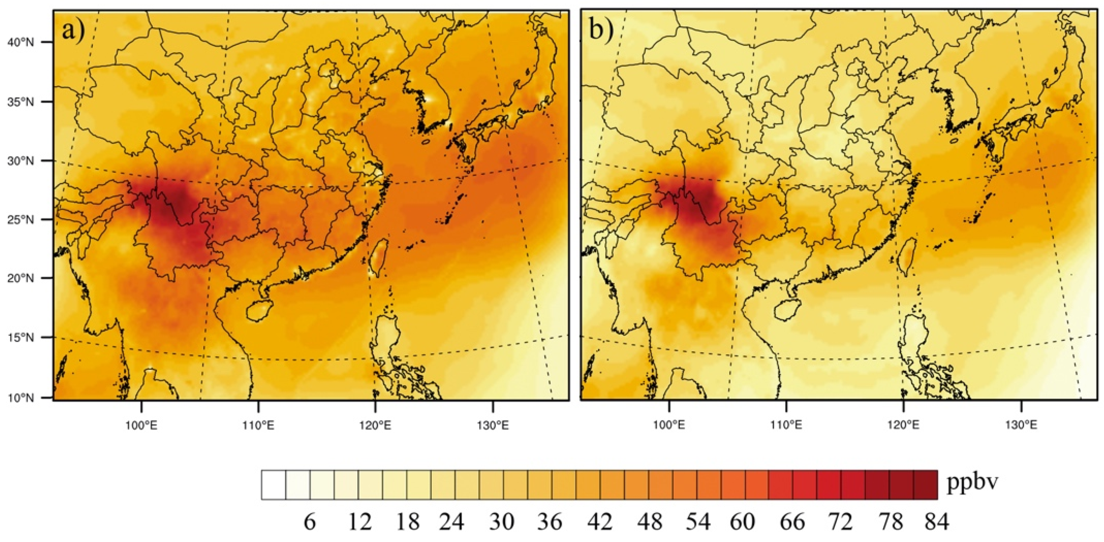
3.3.1. Regional Perspective on Policy Relevant Background Ozone

The base case and EA0 were simulated to provide PRB ozone over EA. Figure 4 shows an example of April’s surface ozone concentrations of the base case and EA0 over the simulation domain. The selection of the April case is to illustrate the situation of high ozone condition in our simulation, which aligns with the objective of finding the PRB ozone over EA. The base case (Figure 4a) with no emission reduction and EA0 (Figure 4b) showed relatively high ozone concentrations between 20° N and 30° N located near the border of Yunnan, Sichuan, and Qinghai (west of China) at the edge of the Tibetan Plateau.
The high average ozone in the mountainous area was attributed to the high background ozone from the boundary conditions. Table S1 shows the GEOS-Chem boundary conditions of all four edges from the study. It is found that the average ozone concentrations aloft at the westbound and northbound in April have reached ~50 ppbv and ~90 ppbv at the 18th (at 5.1 km in altitude), and the model top layers (i.e., layer 26 at about 20.5 km in altitude), respectively. Due to the proximity (both vertical and horizontal) between the high-ozone boundary and ground surface (i.e., ~2–4 km msl), effective transport of ozone from boundary conditions has been found, which was the primary source of background ozone in the westbound and mountainous areas on both base case and EA0. The highest value found in EA0 at the mountainous grids was 84 ppbv, slightly higher than the reported values in Mt. Tai (max: 74 ppbv) [5]. In the north of east Asia, high background ozone with less distinct is found in the oceanic area near East China Sea, Korea, and Japan due to high ozone in the northbound. The CMAQ simulated values in the marine area seem to be slightly overestimated (i.e., ~40 ppbv). Akimoto et al. [35] reported that the low value of dry deposition velocity used in CMAQ might attribute to the overestimation of the ozone mixing ratio in the background oceanic air mass. Overall, the surface concentrations in EA0, excluding the mountainous areas (Figure 4b), ranged between ~20 and 64 ppbv, which seems reasonable. Table 6 shows the summary of monthly ozone from the EA0 scenario under different climatic zones.
Among the climatic zones, Plateau Climate ozone had higher values in most seasons other than January with an annual mean ozone concentration of 37.5 ppbv (based only on four representative months), which was the highest among the eight zones. The high altitude position has resulted in more ozone aloft being received when compared with other regions, as discussed earlier. In addition, the most significant seasonal difference in ozone concentration is found in the mid-subtropical zone. The large range in ozone (43 ppbv) is attributed to the high ozone concentration in April (59 ppbv, which was also the largest one among all zones and seasons) and the small one in July (16 ppbv). On the other hand, the South and mid-temperate zones had the smallest ranges (19 and 14 ppbv) with the smallest mean ozone concentrations (29.3 and 29 ppbv). The mean PRB ozone of all regions is estimated to be 44.8 ppbv for spring and 19.7 ppbv for summer, higher than the values reported by Zhang et al. [8] using GEOS-Chem.

3.3.2. Influence of Stratospheric Ozone Transport on Policy Relevant Background Ozone

Figure 5a shows the contribution of STT to background ozone, where considerable ozone enhancement has been found in both mountainous areas in the westbound and oceanic regions in the northbound. In the mountainous area (i.e., Tibetan Plateau), as the distance between the stratosphere and ground surface is the shortest, effective transport of ozone aloft to the Plateau surface has been detected, causing stronger ozone enhancement from STT. A similar phenomenon was also reported by Emery et al. [6] in spring for the continental US simulations. It was estimated that the STT enhancement in the Plateau climate zone could be as much as 2.2 ppbv (on 19 April 2006) with an average of 0.87 ppbv, which was lower than our expectation. The relatively low ozone enhancement may attribute to the underestimation of ozone aloft from GEOS-Chem boundary conditions [22]. In addition, averaging the STT values from non-uniform enhancement for a large area may result in a smaller average value. Regardless of the situation, large spatial variations of STT enhancement along the Mt. Himalayas have indeed been spotted in the Tibetan Plateau from our simulation, reflecting other factors beyond the influence of altitude (e.g., upper air meteorology) that may have contributed to these variations.
Other locations with considerable STT enhancement were the north and northeast parts of East Asia near Japan and Korea. The ozone enhancement from STT may be attributed to the unstable meteorological condition from the transition between winter and summer monsoons, which intensified the vertical transport of air parcels between the upper and lower atmosphere, driving high ozone aloft from the northbound to the affected areas [36,37,38]. Figure 5b shows the seasonal ozone impacts from STT in the affected area (i.e., Tokyo). Among them, April had the highest ozone enhancement, followed by October, January, and July. Other cities in the north (e.g., Beijing and Seoul) also show similar seasonal patterns (Figure S3b). For the cities in the south, enhancement from STT was a lot weaker than in the cities in the north. As tropopause height is somewhat positively correlated with the ambient temperature, lower STT enhancement is generally expected from the cities with warmer weather (See Figure S3 for two other selected cities). For example, the effect of STT in Guangzhou (i.e., mean value of 0.6 ppbv) was much smaller than in Beijing (i.e., mean value of 2.1 ppbv) for April. The simulated maximum daily enhancement for January, April, July, and October from STT for the entire domain were 3.6 ppbv, 7.5 ppbv, 4.0 ppbv, and 5.6 ppbv, respectively.

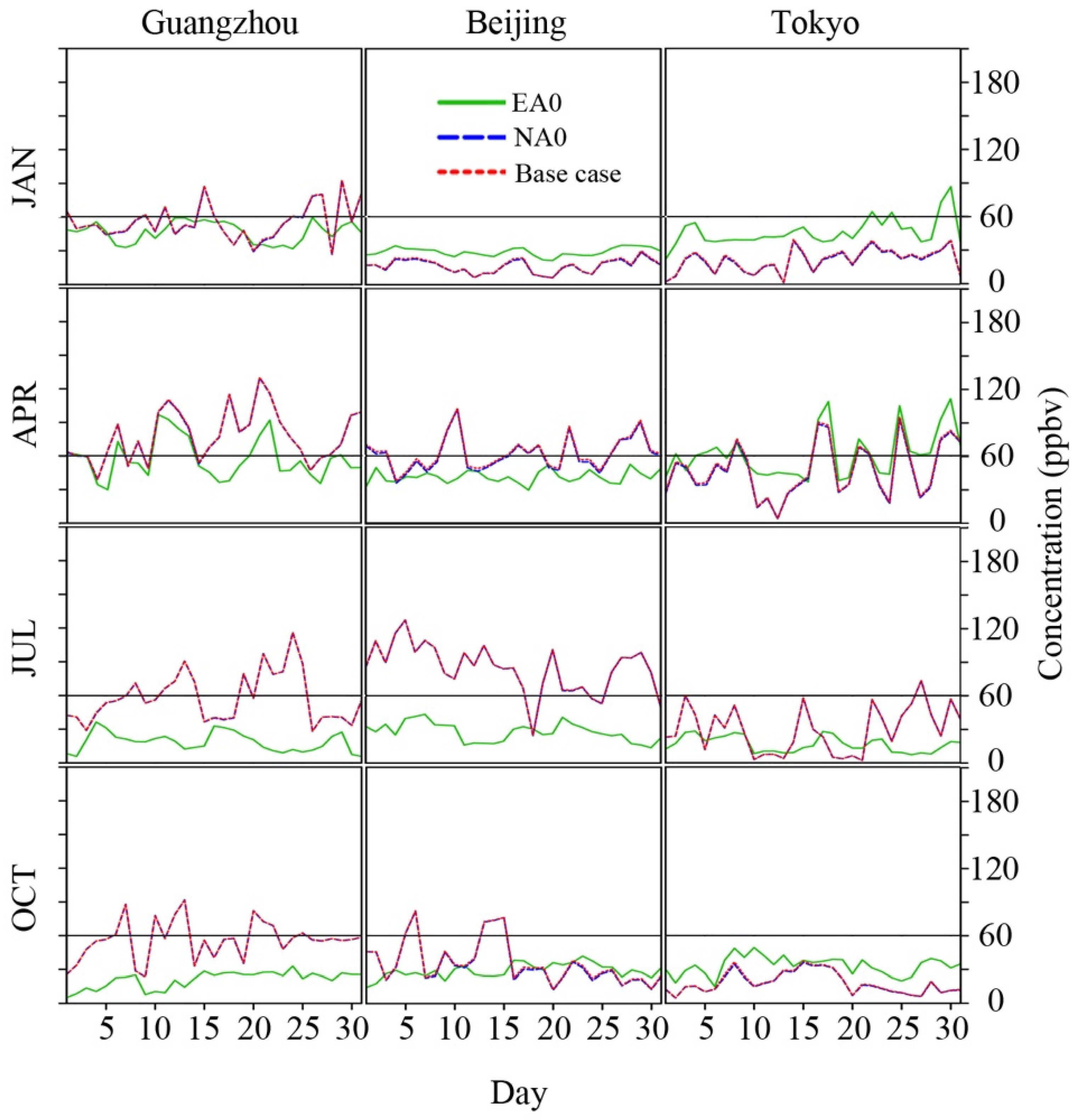
3.3.3. Policy Relevant Background Ozone in Selected Cities

From the perspective of city air quality, Figure 6 shows the time series of three selected cities: Guangzhou, Beijing, and Tokyo (the same cities used for the STT discussion). Note that the time series of the base case (red dotted line) and NA0 (blue dashed line) overlap for all times in the figures.
In January, Beijing and Tokyo had a higher daily average ozone in EA0 than the base case. It indicates that heavy NOx titration with limited photochemical reactions was involved. Among these cities, Tokyo had experienced the strongest NOx titration (as indicated by the difference between the base case and EA0) due to the regional transport of air pollutants from China and Korea. As the temperature in January over the northern part of East Asia was very low, it didn’t encourage photochemistry. So, ozone was relatively low in those two cities. However, in Guangzhou, some ozone production has been detected, and the ozone values in the base case were higher than in EA0. In April, photochemistry started to take place in Beijing. A slight increase in ozone is found in the base case, while Tokyo was still under the same influence from NOx titration with limited photochemistry. The ozone concentration in the base case was still higher than in EA0 for Guangzhou, which was similar to that in January, but with larger magnitudes. In summer (July), all three cities exhibited a positive increase in ozone from EA0 to the base case, attributed to a much lower ozone background in July. In July, the background ozone (EA0) for those cities was consistently low than the regulatory value of 60 ppbv (hourly standard) from the Japanese environmental quality, indicating that reducing anthropogenic emissions could comply with Japan’s ozone regulations. In contrast, the daily background ozone values in April occasionally exceeded the value of 60 ppbv in Tokyo, reflecting that emission reduction may not be sufficient to resolve the high ozone background. In October, the cold weather emerged again, resulting in a similar situation as in January. The ozone concentration in Guangzhou for the base case was always higher than that of EA0. In Beijing, higher ozone concentration is detected in the base case for most days in the first half of October, but it reversed in the second half. For Tokyo, the relationship between the base case and EA0 was similar to that in January, but there was less difference in ozone values between them. The summary of EA0 for the monthly maximum MDA8 ozone from the nine selected cities is shown in Figure 7.
Among the cities, Beijing, Hong Kong, Seoul, Shanghai, and Tianjin had relatively low MDA8 ozone in most seasons, while Chongqing, Guangzhou, Taipei, and Tokyo had high MDA8 ozone. The calculated PRB MDA8 ozone averaged over the nine cities were 53 ppbv for spring (April) and 22 ppbv for summer (July), respectively. Overall, no city has exceeded the Chinese Air Quality Standard of 80 ppbv (160 mg/m3) under the EA0 scenario, indicating that continuing emission reduction in EA would make these cities meet the ozone air quality standard.

4. Conclusions

The CMAQ air quality model was coupled with GEOS-Chem to study the effects of long-range transport and stratospheric ozone transport on policy-relevant background ozone. Overall, large seasonal and spatial variations were found in both LRT and STT impacts. From the perspective of seasons, springtime (i.e., April) has consistently received the highest ozone impacts for near all locations (except the North Tropical zone, the south tip of China). In LRT analysis, the largest effect was spotted in April for the South Temperate zone with the regional average of 1.17 ppbv, while the lowest was in July for the Mid-Subtropical zone (i.e., 0.1 ppbv). For STT, three distinct areas have been identified to have high ozone enhancement: north of the domain, northeastern parts of the domain near Korea and Japan, and southwest of China in the Tibetan Plateaus. The highest enhancement from STT occurred in the Mid-Temperate zone with an average value of 2.17 ppbv, followed by the South Temperate zone (i.e., 1.73 ppbv) and North Subtropical (i.e., 1.10 ppbv). Overall, the ozone enhancement from STT was generally higher than from LRT. Combining the impacts, the influence on monthly background ozone could be as much as 3.6 ppbv, which occurred in the Mid Temperate zone in April. For the analysis of PRB ozone, the maximum daily 8-h ozone from the nine selected cities was all below the Chinese ambient air quality standard of 80 ppbv, indicating that achieving good ozone air quality through anthropogenic emission reduction is possible. Among the cities, Chongqing, Guangzhou, Taipei, and Tokyo had relatively higher PRB ozone in April than the other cities. Extra ~20 ppbv (i.e., PBR ozone at ~60 ppbv) of MDA8 ozone would trigger the exceedance of the ozone air quality standard. It should be aware that all simulated results were based on the 2006 study year. Updating the simulation to more recent years with multi-year simulation would be beneficial in future studies, for which the influence of meteorological variability on PRB ozone as well as the up-to-date emission situation could be accounted. At last, this study has laid essential groundwork for studying PRB ozone in East Asia. The spatial and seasonal relationships of STT defined in this study would less likely be changed in a short time due to the physical constraints (i.e., altitude, latitude and longitude position, and temperature). However, the magnitude of influence will be expected to change because of the projected emission reduction and changing climate. It is recommended that assessment of LRT and STT should be performed at a 5 to 10 years interval to better cope with the rapidly changing world.

Supplementary Materials

The following supporting information can be downloaded at: https://www.mdpi.com/article/10.3390/atmos13050723/s1, Figure S1: GEOS-Chem masking applied for this study: a) zero-out NA (NA0) and b) zero-out EA (EA0); Figure S2: Hourly time series of observation comparison: (a) July at Ryori; (b) October at Ryori; (c) July at Tap Mun, and (d) October at Tap Mun. (e) vertical ozone profile at King’s Park, Hong Kong (22°19′ N 114°10′ E); Figure S3: Ozone enhancement from stratospheric ozone transport: (a) time series for Guangzhou and (b) time series for Beijing. Table S1: Example of monthly averaged boundary ozone concentrations (April).

Author Contributions

Conceptualization, Y.F.L.; model simulation and data management, Y.F.L. and H.M.C.; data analyses, Y.F.L. and H.M.C.; writing—review and editing, Y.F.L. and H.M.C.; funding acquisition, Y.F.L. All authors have read and agreed to the published version of the manuscript.

Funding

This research was funded by the Research Grants Council, University Grants Committee grant number [21300214].

Institutional Review Board Statement

Not applicable.

Acknowledgments

This work was supported by the Research Grants Council, University Grants Committee [21300214]. The author would like to acknowledge the Hong Kong Environmental Protection Department for providing emission inputs. We thank Daniel Jacob at Harvard University for providing the GEOS-Chem outputs. The computations were partially performed using research computing facilities offered by Information Technology Services, the University of Hong Kong.

Conflicts of Interest

The authors declare no conflict of interest.

References

  1. USEPA. Health Risk and Exposure Assessment for Ozone; U.S. Environmental Protection Agency: Washington, DC, USA, 2014.
  2. McDonald-Buller, E.C.; Allen, D.T.; Brown, N.; Jacob, D.J.; Jaffe, D.; Kolb, C.E.; Lefohn, A.S.; Oltmans, S.; Parrish, D.D.; Yarwood, G.; et al. Establishing Policy Relevant Background (PRB) Ozone Concentrations in the United States. Environ. Sci. Technol. 2011, 45, 9484–9497. [Google Scholar] [CrossRef]
  3. CRS. Background Ozone: Challenges in Science and Policy; CRS: Washington, DC, USA, 2019. [Google Scholar]
  4. Li, J.; Wang, Z.; Akimoto, H.; Gao, C.; Pochanart, P.; Wang, X. Modeling study of ozone seasonal cycle in lower troposphere over east Asia. J. Geophys. Res. Atmos. 2007, 112, D22S25. [Google Scholar] [CrossRef]
  5. Ou Yang, C.-F.; Lin, N.-H.; Sheu, G.-R.; Lee, C.-T.; Wang, J.-L. Seasonal and diurnal variations of ozone at a high-altitude mountain baseline station in East Asia. Atmos. Environ. 2012, 46, 279–288. [Google Scholar] [CrossRef]
  6. Emery, C.; Jung, J.; Downey, N.; Johnson, J.; Jimenez, M.; Yarwood, G.; Morris, R. Regional and global modeling estimates of policy relevant background ozone over the United States. Atmos. Environ. 2012, 47, 206–217. [Google Scholar] [CrossRef]
  7. Hogrefe, C.; Henderson, B.; Tonnesen, G.; Mathur, R.; Matichuk, R. Multiscale Modeling of Background Ozone: Research Needs to Inform and Improve Air Quality Management. EM Magazine, 1 November 2020; 1–6. [Google Scholar]
  8. Zhang, L.; Jacob, D.J.; Downey, N.V.; Wood, D.A.; Blewitt, D.; Carouge, C.C.; van Donkelaar, A.; Jones, D.B.A.; Murray, L.T.; Wang, Y. Improved estimate of the policy-relevant background ozone in the United States using the GEOS-Chem global model with 1/2° × 2/3° horizontal resolution over North America. Atmos. Environ. 2011, 45, 6769–6776. [Google Scholar] [CrossRef] [Green Version]
  9. Aijun, D.; Tao, W.; Likun, X.; Jian, G.; Andreas, S.; Hengchi, L.; Dezhen, J.; Yu, R.; Xuezhong, W.; Xiaolin, W.; et al. Correction to “Transport of north China air pollution by midlatitude cyclones: Case study of aircraft measurements in summer 2007”. J. Geophys. Res. Atmos. 2009, 114, D11399. [Google Scholar] [CrossRef] [Green Version]
  10. Husar, R.B.; Tratt, D.M.; Schichtel, B.A.; Falke, S.R.; Li, F.; Jaffe, D.; Gassó, S.; Gill, T.; Laulainen, N.S.; Lu, F.; et al. Asian dust events of April 1998. J. Geophys. Res. Atmos. 2001, 106, 18317–18330. [Google Scholar] [CrossRef]
  11. Isaac, T.B.; Daniel, A.J. Long-range transport of ozone, carbon monoxide, and aerosols to the NE Pacific troposphere during the summer of 2003: Observations of smoke plumes from Asian boreal fires. J. Geophys. Res. Atmos. 2005, 110, D05303. [Google Scholar] [CrossRef]
  12. Derwent, R.G.; Jenkin, M.E. Hydrocarbons and the long-range transport of ozone and pan across Europe. Atmos. Environ. Part A Gen. Top. 1991, 25, 1661–1678. [Google Scholar] [CrossRef]
  13. Fischer, E.V.; Jacob, D.J.; Yantosca, R.M.; Sulprizio, M.P.; Millet, D.B.; Mao, J.; Paulot, F.; Singh, H.B.; Roiger, A.; Ries, L.; et al. Atmospheric peroxyacetyl nitrate (PAN): A global budget and source attribution. Atmos. Chem. Phys. 2014, 14, 2679–2698. [Google Scholar] [CrossRef] [Green Version]
  14. Nielsen, T.; Samuelsson, U.; Grennfelt, P.; Thomsen, E.L. Peroxyacetyl nitrate in long-range transported polluted air. Nature 1981, 293, 553–555. [Google Scholar] [CrossRef]
  15. Lin, C.-Y.; Zhao, C.; Liu, X.; Lin, N.-H.; Chen, W.-N. Modelling of long-range transport of Southeast Asia biomass-burning aerosols to Taiwan and their radiative forcings over East Asia. Tellus B 2014, 66, 23733. [Google Scholar] [CrossRef] [Green Version]
  16. Fu, J.S.; Dong, X.; Gao, Y.; Wong, D.C.; Lam, Y.F. Sensitivity and linearity analysis of ozone in East Asia: The effects of domestic emission and intercontinental transport. J. Air Waste Manag. Assoc. 2012, 62, 1102–1114. [Google Scholar] [CrossRef] [PubMed] [Green Version]
  17. Lee, Y.C.; Lam, Y.F.; Kuhlmann, G.; Wenig, M.O.; Chan, K.L.; Hartl, A.; Ning, Z. An integrated approach to identify the biomass burning sources contributing to black carbon episodes in Hong Kong. Atmos. Environ. 2013, 80, 478–487. [Google Scholar] [CrossRef]
  18. Wang, M.; Fu, Q. Stratosphere-Troposphere Exchange of Air Masses and Ozone Concentrations Based on Reanalyses and Observations. J. Geophys. Res. Atmos. 2021, 126, e2021JD035159. [Google Scholar] [CrossRef]
  19. Griffiths, P.T.; Murray, L.T.; Zeng, G.; Shin, Y.M.; Abraham, N.L.; Archibald, A.T.; Deushi, M.; Emmons, L.K.; Galbally, I.E.; Hassler, B.; et al. Tropospheric ozone in CMIP6 simulations. Atmos. Chem. Phys. 2021, 21, 4187–4218. [Google Scholar] [CrossRef]
  20. Lin, M.; Fiore, A.M.; Cooper, O.R.; Horowitz, L.W.; Langford, A.O.; Levy Ii, H.; Johnson, B.J.; Naik, V.; Oltmans, S.J.; Senff, C.J. Springtime high surface ozone events over the western United States: Quantifying the role of stratospheric intrusions. J. Geophys. Res. Atmos. 2012, 117, D00V22. [Google Scholar] [CrossRef] [Green Version]
  21. Itahashi, S.; Mathur, R.; Hogrefe, C.; Zhang, Y. Modeling stratospheric intrusion and trans-Pacific transport on tropospheric ozone using hemispheric CMAQ during April 2010—Part 1: Model evaluation and air mass characterization for stratosphere–troposphere transport. Atmos. Chem. Phys. 2020, 20, 3373–3396. [Google Scholar] [CrossRef] [Green Version]
  22. Lam, Y.F.; Fu, J.S. Corrigendum to “A novel downscaling technique for the linkage of global and regional air quality modeling”. Atmos. Chem. Phys. 2009, 9, 9169–9185. Atmos. Chem. Phys. 2010, 10, 4013–4031. [Google Scholar] [CrossRef] [Green Version]
  23. Environ. Upgrade of a Regional Air Quality Modelling System (PATH)—Feasibility Study; ENVIRON Hong Kong Limited: Hong Kong, China, 2011. [Google Scholar]
  24. Holmes, C.D.; Jacob, D.J.; Corbitt, E.S.; Mao, J.; Yang, X.; Talbot, R.; Slemr, F. Global atmospheric model for mercury including oxidation by bromine atoms. Atmos. Chem. Phys. 2010, 10, 12037–12057. [Google Scholar] [CrossRef] [Green Version]
  25. Selin, N.E.; Daniel, J.J.; Robert, M.Y.; Sarah, S.; Lyatt, J.; Elsie, M.S. Global 3-D land-ocean-atmosphere model for mercury: Present-day versus preindustrial cycles and anthropogenic enrichment factors for deposition. Glob. Biogeochem. Cycles 2008, 22, GB2011. [Google Scholar] [CrossRef]
  26. Zhang, Q.; Streets, D.G.; Carmichael, G.R.; He, K.B.; Huo, H.; Kannari, A.; Klimont, Z.; Park, I.S.; Reddy, S.; Fu, J.S.; et al. Asian emissions in 2006 for the NASA INTEX-B mission. Atmos. Chem. Phys. 2009, 9, 5131–5153. [Google Scholar] [CrossRef] [Green Version]
  27. Lam, Y.F.; Fu, J.S.; Wu, S.; Mickley, L.J. Impacts of future climate change and effects of biogenic emissions on surface ozone and particulate matter concentrations in the United States. Atmos. Chem. Phys. 2011, 11, 4789–4806. [Google Scholar] [CrossRef] [Green Version]
  28. CESY. China Electricity Statistical YearBook 2005; National Bureau of Statistics of China: Beijing, China, 2005; p. 42.
  29. Huang, K.; Fu, J.S.; Hsu, N.C.; Gao, Y.; Dong, X.; Tsay, S.-C.; Lam, Y.F. Impact assessment of biomass burning on air quality in Southeast and East Asia during BASE-ASIA. Atmos. Environ. 2013, 78, 291–302. [Google Scholar] [CrossRef] [Green Version]
  30. Streets, D.G.; Bond, T.C.; Carmichael, G.R.; Fernandes, S.D.; Fu, Q.; He, D.; Klimont, Z.; Nelson, S.M.; Tsai, N.Y.; Wang, M.Q.; et al. An inventory of gaseous and primary aerosol emissions in Asia in the year 2000. J. Geophys. Res. Atmos. 2003, 108, 23. [Google Scholar] [CrossRef]
  31. Du, Y.; Lam, Y.F.; Fu, J.S. Top-down emission inventory development for INTEX-B. In Proceedings of the A&WMA’s 101th Annual Conference, Detroit, MI, USA, 16–19 June 2009. [Google Scholar]
  32. Lam, Y.F.; Cheung, C.C.; Zhang, X.; Fu, J.S.; Fung, J.C.H. Development of a new emission reallocation method for industrial sources in China. Atmos. Chem. Phys. 2021, 21, 12895–12908. [Google Scholar] [CrossRef]
  33. Hakami, A.; Henze, D.K.; Seinfeld, J.H.; Chai, T.; Tang, Y.; Carmichael, G.R.; Sandu, A. Adjoint inverse modeling of black carbon during the Asian Pacific Regional Aerosol Characterization Experiment: Adjoint Inverse Modeling of Black Carbon. J. Geophys. Res. Atmos. 2005, 110, 1–17. [Google Scholar] [CrossRef] [Green Version]
  34. Sartelet, K.N.; Hayami, H.; Sportisse, B. MICS Asia Phase II—Sensitivity to the aerosol module. Atmos. Environ. 2008, 42, 3562–3570. [Google Scholar] [CrossRef] [Green Version]
  35. Akimoto, H.; Nagashima, T.; Kawano, N.; Jie, L.; Fu, J.S.; Wang, Z. Discrepancies between MICS-Asia III simulation and observation for surface ozone in the marine atmosphere over the northwestern Pacific Asian Rim region. Atmos. Chem. Phys. 2020, 20, 15003–15014. [Google Scholar] [CrossRef]
  36. Kim, J.H.; Lee, H.J.; Lee, S.H. The Characteristics of Tropospheric Ozone Seasonality Observed from Ozone Soundings at Pohang, Korea. Environ. Monit. Assess. 2006, 118, 1–12. [Google Scholar] [CrossRef]
  37. Hwang, S.-H.; Kim, J.; Cho, G.-R. Observation of secondary ozone peaks near the tropopause over the Korean peninsula associated with stratosphere-troposphere exchange. J. Geophys. Res. Atmos. 2007, 112, D16305. [Google Scholar] [CrossRef] [Green Version]
  38. Kalabokas, P.; Hjorth, J.; Foret, G.; Dufour, G.; Eremenko, M.; Siour, G.; Cuesta, J.; Beekmann, M. An investigation on the origin of regional springtime ozone episodes in the western Mediterranean. Atmos. Chem. Phys. 2017, 17, 3905–3928. [Google Scholar] [CrossRef] [Green Version]
Figure 1. CMAQ simulation domain (D1–27 km) with defined climatic zones and selected cities.
Atmosphere 13 00723 g001
Figure 2. Hourly time series of observation comparison: (a) January at Ryori, (b) April at Ryori, (c) January at Tap Mun, and (d) April at Tap Mun. Daily mean scatter plots for model vs observation: (e) Ryori and (f) Tap Mun.
Atmosphere 13 00723 g002
Figure 3. Ozone enhancement (base case-NA0) of long-range transport from North America.
Atmosphere 13 00723 g003
Figure 4. Monthly average ozone for April: (a) Base case and (b) EA0.
Atmosphere 13 00723 g004
Figure 5. Ozone enhancement from stratospheric ozone transport: (a) average value in April and (b) time series for Tokyo.
Atmosphere 13 00723 g005
Figure 6. Daily average ozone time series for CMAQ simulated cases. The black line indicates the Japanese environmental quality standards of 60 ppbv.
Atmosphere 13 00723 g006
Figure 7. Monthly maximum MDA8 ozone concentrations from EA0 scenario for nine selected cities.
Atmosphere 13 00723 g007
Table 1. Multi-emission scenarios used in GEOS-Chem.
Case NameDescriptionRemoved Emissions 1
Full EMBase case with no emissions reduction-
Zero-out EARemove East Asia’s emissionsSTREETS (all pollutants)
Zero-out NARemove North America’s emissionsNEI 05 for US, CAC for Canada & BRAVO for Mexico
1 NEI05-National Emissions Inventory in 2005, CAC-Criteria Air Contaminants inventory, BRAVO-Emissions inventory developed through BRAVO study, and STREETS-Emissions inventory developed by Zhang et al. [26] via INTEX-B experiment.
Table 2. Configuration of CMAQ air quality simulation.
ConfigurationOptions
Model CodeCMAQ Version 5.0.1
Horizontal Grid MeshD1–27 km
(East Asia)
Vertical Grid Mesh34 Layers
Grid InteractionOne-way nesting
Initial/Boundary ConditionGEOS-Chem global chemistry model
Emissions
Emissions ProcessingINTEX-B with a top-down approach [26,31]
Sub-grid-scale PlumesNo PinG
Chemistry
Gas-Phase ChemistryCB05
Aerosol ChemistryAE4/ISORROPIA
Secondary Organic AerosolsSORGAM
Cloud ChemistryRADM
Horizontal Transport
Eddy DiffusivityK-theory
Vertical Transport
Eddy DiffusivityACM2
Deposition SchemeM3Dry
Numeric
Gas-Phase Chemistry SolverEBI
Horizontal Advection SchemePPM
Table 3. Summary of scenarios applied in CMAQ simulation.
Scenario NameGEOS-Chem Initial & Boundary Conditions
(Case Name)
CMAQ Emission
Description
Base caseFull Global emissions, including anthropogenic + biogenic + biomass burning (Full EM)All emissions from the PATH system (including biogenic, biomass burning, etc.)
NA0Removal of NEI05, CAC and BRAVO emissions from global inventory (Zero-out NA)All emissions from the PATH system (including biogenic, biomass burning, etc.)
EA0Removal of STREETS (all pollutants) from global inventory (Zero-out EA)Removal of all anthropogenic (INTEX-B and TRACE-P Ship) emissions from the CMAQ domain
STTEA0 with the removal of stratospheric ozone from the upper level of GEO-Chem input (Zero-out EA) Removal of all anthropogenic (INTEX-B and TRACE-P Ship) emissions from the CMAQ domain
Table 4. Summary of statistical results on surface observation comparison.
MonthRyori, Japan
(39°02′ N 141°49′ E)
Tap Mun, Hong Kong
(22°28′ N 114°21′ E)
Mean(Obs)Mean(Model)MBMAERMSEMean (Obs)Mean (Model)MBMAERMSE
January37.638.5+0.84.35.831.852.2+21.125.328.9
April49.049.6+0.79.011.929.348.8+21.826.533.3
July31.832.9+1.112.815.222.727.5+5.213.417.9
October40.237.0−2.811.214.849.551.3+2.716.122.3
Note: Obs–observation; Model–model output; MB–Mean Bias; MAE–Mean Absolute Error; RMSE–Root Mean Square Error.
Table 5. Ozone influence over EA resulted from NA emissions.
Month
(ppbv)
South
Temperate
Plateau
Climate
North
Subtropical
North
Tropical
Mid
Subtropical
Mid
Temperate
South
Subtropical
JAN0.830.440.670.37 10.490.850.43
APR1.17 10.61 10.76 10.280.60 11.47 10.44 1
JUL0.160.150.080.240.100.320.16
OCT0.680.590.440.190.260.830.18
1 Highest value from each climatic zone.
Table 6. Monthly ozone concentrations from the EA0 scenario for seven climatic zones.
Month
(ppbv)
South
Temperate
Plateau ClimateNorth
Subtropical
North TropicalMid
Subtropical
Mid
Temperate
South
Subtropical
Avg.
JAN31 (2)35 (13)35 (5)46 (14)37 (16)28 (5)39 (13)35.8
APR39 1 (15)50 1 (9)44 1 (21)37 1 (15)59 1 (20)38 1 (10)47 1 (16)44.8 1
JUL20 (25)27 (12)15 (27)20 (13)16 (22)24 (20)16 (16)19.7
OCT27 (13)38 (10)26 (19)25 (30)27 (22)26 (10)23 (21)27.4
1 Highest value from each climatic zone. Value in the bracket reflects the difference in ozone concentration between the base case and EA0 (i.e., base case–EA0).
Publisher’s Note: MDPI stays neutral with regard to jurisdictional claims in published maps and institutional affiliations.

