Parametrization of Horizontal and Vertical Transfers for the Street-Network Model MUNICH Using the CFD Model Code_Saturne

Abstract

Cities are heterogeneous environments, and pollutant concentrations are often higher in streets compared with in the upper roughness sublayer (urban background) and cannot be represented using chemical-transport models that have a spatial resolution on the order of kilometers. Computational Fluid Dynamics (CFD) models coupled to chemistry/aerosol models may be used to compute the pollutant concentrations at high resolution over limited areas of cities; however, they are too expensive to use over a whole city. Hence, simplified street-network models, such as the Model of Urban Network of Intersecting Canyons and Highways (MUNICH), have been developed. These include the main physico-chemical processes that influence pollutant concentrations: emissions, transport, deposition, chemistry and aerosol dynamics. However, the streets are not discretized precisely, and concentrations are assumed to be homogeneous in each street segment. The complex street micro-meteorology is simplified by considering only the vertical transfer between the street and the upper roughness sublayer as well as the horizontal transfer between the streets. This study presents a new parametrization of a horizontal wind profile and vertical/horizontal transfer coefficients. This was developed based on a flow parametrization in a sparse vegetated canopy and adapted to street canyons using local-scale simulations performed with the CFD model Code_Saturne. CFD simulations were performed in a 2D infinite street canyon, and three streets of various aspect ratios ranging from $0.3$ to $1.0$ were studied with different incoming wind directions. The quantities of interest (wind speed in the street direction and passive tracer concentration) were spatially averaged in the street to compare with MUNICH. The developed parametrization depends on the street characteristics and wind direction. This effectively represents the average wind profile in a street canyon and the vertical transfer between the street and the urban roughness sublayer for a wide range of street aspect ratios while maintaining a simple formulation.

1. Introduction

Cities are areas of highly concentrated human activities that induce large amounts of air pollutants emitted by anthropic activities, such as traffic, industry and residential activities. Cities are also heterogeneous environments, and the presence of high buildings represents obstacles that reduce air flow inside streets and limit the dispersion of pollutants emitted within [1,2,3,4]. These two processes lead to poor air quality, thus, imposing a risk for human health. In addition, the growing number of people living in cities increases the vulnerability, and massive urbanization has negative consequences on the environment and human health especially during pollution peaks [5,6,7,8,9]. In the case of a street canyon, air recirculates inside the canyon, as shown by Harman et al. [10] for the wind perpendicular to the street.

Pollutants emitted in the street—by traffic for example—tend to accumulate on the leeward side of the street, and the concentrations at this location may be much higher than the background concentrations [11,12,13]. Knowing that people spend most of their time indoors, the vertical distribution of pollutant concentrations is also a key research topic. People are not only exposed to air pollution at street pedestrian level but also to air pollution inside buildings, which may be influenced by outdoor pollution and the height levels of the building [14,15,16].

Models are powerful tools to study air flow and pollutant concentration because the conditions can be fixed and the simulations are easily replicable, thus, allowing the analysis of different processes influencing the concentrations. Currently, chemistry-transport models (CTMs) are widely used at the meso-scale to understand processes, interpret observations and forecast the evolution of pollutant concentrations [17,18,19,20]. Informed by emissions inventories, meteorological, initial and boundary conditions, these models use numerical techniques to simulate pollutant transport, chemical transformation in the atmosphere and compute air concentrations and deposition fluxes.

In CTMs, concentrations are averaged over mesh cells with a horizontal resolution ranging from kilometers to hundreds of kilometers. Due to their coarse spatial resolution, CTMs are not able to capture the high pollutant concentrations observed in streets, and thus city-scale models, such as simplified street-network or street-in-grid models are used to represent the street level concentrations [21,22,23,24,25,26].

Street models use parametrizations to represent the dispersion of pollutants at the street level over a neighborhood or a city. The streets are not discretized finely; however, concentrations are assumed to be homogeneous in each street segment, as in the Model of Urban Network of Intersecting Canyons and Highways (MUNICH) [24,25], or in part of the street (lee side versus wind side, for example, as in the OSPM (Operational Street Pollution Model) [21].

To study wind fields and pollutant dispersion at a local scale (100 m to 1 km), Computational Fluid Dynamics (CFD) are commonly used [27,28,29]. The simulation domain is composed of grid cells with a resolution ranging from centimeters to meters. To solve air flow in two or three dimensions, several turbulence schemes are used, such as $k-\epsilon$ and Large Eddy Simulation (LES). This type of model allows capturing the complex street micro-meteorology; however, the computational cost is high to study pollutant dispersion at city scale as this requires billions of grids.

As concentrations are assumed to be homogeneous in each street segment, the computational cost associated with MUNICH is low compared to CFD, allowing simulations over a whole city [25]. To model the dispersion of pollutants, the street-network model MUNICH separates air flow into two components related to transfer velocities. First, the horizontal wind speed is assumed to follow the street direction and to be homogeneous across the street. Second, the vertical transfer velocity between the street and the background domain is calculated at the roof level.

These horizontal and vertical air flows depend on the canyon geometry, wind angle, above-street flow and atmospheric stability [30]. Background concentrations above the roughness sublayer can be provided by 3D CTMs, such as Polair3D from the Polyphemus air-quality modeling platform [25,26,31].

The objective of this study is to evaluate the parametrizations that are currently used in MUNICH for the horizontal and vertical transfers as well as to develop a new parametrization as accurate as the existing ones but with a simpler formulation. It is an adaptation of a parametrization originally designed to model flows in sparse and dense vegetated canopies, depending on the leaf area or spacing between trees. The parametrizations are evaluated by comparisons to Computational Fluid Dynamics (CFD) simulations in street canyons.

They are performed with Code_Saturne [32], an open-source code that can represent air and pollutant flows in a street canyon [33]. “It solves the Navier–Stokes equations for 2D, 2D-axisymmetric and 3D flows, steady or unsteady, laminar or turbulent, incompressible or weakly compressible, isothermal or not, with scalars transport” if required (https://www.code-saturne.org/, accessed on 17 December 2021).

This code has been adapted to atmospheric flows and can simulate the humid atmosphere with radiative heat transfer (not used here). Code_Saturne has been evaluated with the results of the Mock Urban Setting Test (MUST). This is a near full-scale experiment conducted in Utah’s West Desert area based on the release of a neutral gas in a field of regularly spaced shipping containers [33,34]. In addition, Code_Saturne was used to simulate thermal effect and pollutant dispersion in a real urban neighborhood of Toulouse, France [35] and micro-scale heterogeneities of turbulent variables for different wind directions over a complex semi-urban area located near Paris [36].

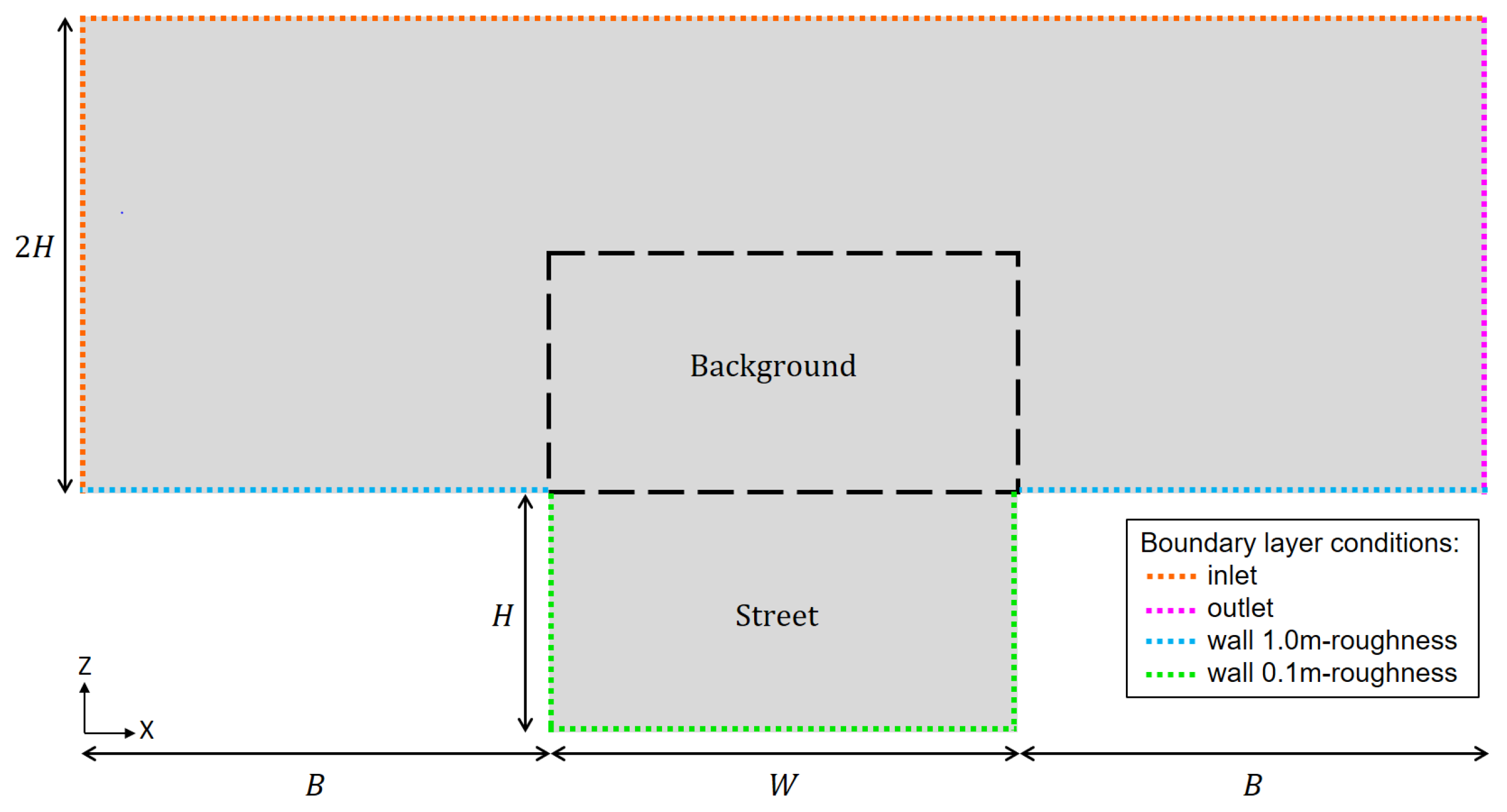
In these different studies, the simulated air flow agreed well with the measurements, demonstrating that Code_Saturne was able to accurately simulate airflow and pollutant dispersion over complex urban sites, as well as 2D simplified street canyons. In the present study, Code_Saturne version 6.0 is used. To compare the parametrizations, several simulations are performed with Code_Saturne to consider different street sizes and wind directions. Therefore, the set-up of the model is simplified, and 2D streets are considered to be consistent with the street-network-model approach.

The structure of the paper is as follows. The models MUNICH and Code_Saturne are detailed in Section 2. Then, a new parametrization for horizontal and vertical transfers based on Code_Saturne simulations and Wang [37,38] is proposed for MUNICH and is compared with existing MUNICH parametrizations in Section 3. Our conclusions are provided in Section 4.

2. Materials and Methods

This section first describes the street-network model MUNICH and then the CFD simulations performed with Code_Saturne.

2.1. Description of MUNICH

2.1.1. Street Geometry and Main Hypothesis

As detailed in Kim et al. [24] and Lugon et al. [25], the streets correspond to the volume of the urban canopy, and each street segment is defined by a length L, uniform street width W and height of the buildings H. Each segment is characterized by its aspect ratio calculated as $a_r=\frac{H}{W}$. Air pollutant concentrations are assumed to be homogeneous within each street segment. The wind in the street follows the street direction and determines the advective air flow, which transports pollutants horizontally. They are also transported in and out of the street network by vertical transfer at the top (roof level) of each street segment. The streets are linked to the background concentrations above roof level by a vertical transfer coefficient. Note that the horizontal wind speed and direction may differ from one street segment to another.

2.1.2. MUNICH Existing Parametrizations for Vertical Transfers

The vertical mass vertical flux of pollutants at the roof level is calculated based on a turbulent transfer coefficient [24,39]:

$$Q_{vert}=q_{vert}WL\frac{\left(C_{street}-C_{bg}\right)}{H}\mathrm{with}{q}_{vert}={\sigma }_W{l}_m$$

(1)

where $Q_{vert}$ is the vertical flux of pollutants at the roof level for the whole street (μg·s⁻¹), $q_{vert}$ is the vertical transfer coefficient (m${}^2$·s${}^{-1}$) and $WL$ is the exchange surface (m${}^2$). $C_{street}$ and $C_{bg}$ are, respectively, the average street and background air pollutant concentrations (μg·m⁻³). $l_m$ is the mixing length within the street (m), and ${\sigma }_W$ is a velocity scale corresponding to the standard deviation of the vertical wind velocity at roof level (m·s${}^{-1}$). ${\sigma }_W$ is function of the atmosphere stability and the friction velocity above the street $u_{*}$ (m·s${}^{-1}$), and is calculated for a neutral atmosphere as [22,40]:

$${\sigma }_W=1.3u_{*}\times \left(1-0.8\frac{H}{PBLH}\right)$$

(2)

$u_{*}$ is not computed by MUNICH but is taken as an input data and is equal to the Code_Saturne friction velocity in the present study (Equation (16)). $PBLH$, also an input, is the planetary boundary layer height (m), which is set to 1000 m in the present simulations [41,42]. The ${\sigma }_W$ parametrizations for stable and unstable atmospheric conditions can be found in Soulhac et al. [22]. The mixing length is assumed to be constant in the street and can be computed in MUNICH either from the Schulte et al. [39] or Soulhac et al. [22] parametrizations:

$$l_m=\frac{DH}{1+a_r}$$

(3)

for Schulte et al. [39],

$$l_m=\frac{H}{\sqrt{2}\pi }$$

(4)

for Schulte et al. [22].

D is a constant equal to $\frac{2}{\sqrt{2}\pi }$ fixed by assuming that the estimation of $l_m$ from the formulations Schulte et al. [39] and Soulhac et al. [22] are equal for $a_r=1$ [24]. Hereafter, to be able to compare these mixing length parametrizations, they are noted L_sch for Schulte et al. [39] and L_sir for Soulhac et al. [22].

2.1.3. MUNICH Existing Parametrizations for Horizontal Transfers

The horizontal flux of pollutants between the streets, $Q_{in/outflow}$ (μg·s⁻¹), is computed in MUNICH as the product of the average wind speed in the street direction $U_{street}$ (m·s${}^{-1}$), which can be interpreted as a horizontal transfer velocity, the exchange section $HW$ (m${}^2$) and the average pollutant concentration in the street $C_{street}$ (μg·m⁻³). Depending on the wind angle $\phi$ (angle between the wind direction and the street orientation), this flux can be an incoming or outgoing flux:

$$Q_{in/outflow}=U_{street}HW{C}_{street}$$

(5)

Two different $U_{street}$ parametrizations already exist in MUNICH.

-

Exponential attenuation profile (noted U_exp)

This profile is an empirical parametrization computed from an exponential attenuation of the wind speed at the roof level and is inspired by wind profiles in vegetated canopies. The wind profile is fully dependent on an attenuation coefficient. The higher the attenuation coefficient, the higher the decrease of the wind speed with altitude. Masson [43], Lemonsu et al. [44] and Cherin et al. [45] proposed an attenuation coefficient of $A\times a_r$, where A is a dimensionless constant equal to 0.5 for wind within street canyons. The value of this attenuation coefficient is tested in Section 3.3.2.

Only advection along the street (i.e., the horizontal component of the wind speed in the street direction) is considered in MUNICH (noted $U_Y$). Therefore, the wind profile is multiplied by $|cos\left(\phi \right)|$ to select only this component. The exponential profile is computed as (modified from Kim et al. [24]):

$$U_Y\left(z\right)=U_{H,\phi }exp\left[A{a}_r\left(\frac{z}{H}-1\right)\right]\forall a_r\mathrm{with}{U}_{H,\phi }=U_H|cos\left(\phi \right)|,$$

(6)

where $U_H$ is the norm of the horizontal wind speed at the building height H (m·s${}^{-1}$), which can be calculated either from Macdonald et al. [46] and Grimmond and Oke [47] or Soulhac et al. [22], z is the vertical elevation (m) (upward orientation and $z=0$ at the ground level), $A{a}_r$ corresponds to the dimensionless attenuation coefficient.

In MUNICH, the average wind velocity in the street ($U_{street}$) is obtained by analytically integrating the wind profile between the soil roughness $z_{0_s}$ (m) and the building height H (m) as:

$${\displaystyle U_{street}={\int }_{z_{0_s}}^H{U}_Y\left(z\right)\mathrm{d}z=U_{H,\phi }\times \frac{1}{A{a}_r}\left(1-exp\left[A{a}_r\left(\frac{z_{0_s}}{H}-1\right)\right]\right)}$$

(7)

-

SIRANE profile (noted U_sir)

Soulhac et al. [22,48] developed an analytical solution of the momentum equation in a street canyon by dividing the canyon into two parts: the region influenced by the walls and the region influenced by the ground. In the region influenced by the walls (in the upper part of the canyon), the horizontal and vertical variations of U are separated and, respectively, represented by the functions f and h. h is a function of z and f is function of x, the horizontal distance with a rightward orientation and $x=0$ at the left wall level of the street (a different reference is used in Code_Saturne because the wind profile is also defined above the buildings, see Section 2.2.1). In the region influenced by the ground, the walls have no influence on the wind profile; however, the wind speed at $z=\delta$ and at all x is taken to ensure the match between the profiles of the two regions.

In the region influenced by the walls ($\delta \le z\le H$ and $z_{0_s}\le x\le W-z_{0_s}$):

$$\begin{array}{cc}\hfill & U(x,z)=U_{m}f(x/\delta )h(z/\delta )\hfill \end{array}$$

(8)

$$\begin{array}{cc}\hfill & f(x/\delta )=\frac{J_1\left(C\right)Y_0(Cx/\delta )-J_0(Cx/\delta )Y_1\left(C\right)}{J_1\left(C\right)Y_0\left(C\right)-J_0\left(C\right)Y_1\left(C\right)}\hfill \end{array}$$

(9)

$$\begin{array}{cc}\hfill & h(z/\delta )=exp\left[\frac{C}{\sqrt{2}}\left(\frac{z-H}{\delta }\right)\right]\hfill \end{array}$$

(10)

In the region influenced by the ground ($z_{0_s}\le z<\delta$ and $z_{0_s}\le x\le W-z_{0_s}$):

$$\begin{array}{cc}\hfill & U(x,z)=U(x,\delta )\times \frac{ln\left(\frac{z}{z_{0_s}}\right)}{ln\left(\frac{\delta }{z_{0_s}}\right)}\hfill \end{array}$$

(11)

$$\begin{array}{cc}\hfill & \mathrm{with}U(x,\delta )=U_{m}f(x/\delta )exp\left[\frac{C}{\sqrt{2}}\left(\frac{\delta -H}{\delta }\right)\right]\hfill \end{array}$$

(12)

where $J_0$, $J_1$, $Y_0$ and $Y_1$ are the first and second kind Bessel functions of order 0 and 1. Unlike U_exp, the SIRANE profile is not calculated from the average wind speed at $z=H$, $U_H$ and, instead, from the wind speed at the top of the street in the middle, $U_m$ (at $z=H$ and $x=W/2$). $U_m$ is determined from the shear stress and friction velocity values at $z=H$. Knowing the wall roughness $z_{0_s}$, C has to be determined by an iterative method (see Equation (14) with $\gamma$ as the Euler constant equal to 0.577).

The wind profile is then integrated in each region of the canyon to compute the average horizontal wind speed in the street [22,24,48]:

$$U_{street}=U_m|cos\left(\phi \right)|\frac{{\delta }^2}{HW}\left[\frac{2\sqrt{2}}{C}\left(1-B_2\right)\left(1-\frac{C^2}{3}+\frac{C^4}{45}\right)+B_2\frac{2B_1-3}{B_1}+\left(\frac{W}{\delta }-2\right)\frac{B_1-1}{B_1}\right]$$

(13)

$$\mathrm{with}\left\{\begin{array}{cc}\hfill & B_1=ln\left(\frac{\delta }{z_{0_s}}\right)\hfill \\ \hfill & B_2=exp\left[\frac{C}{\sqrt{2}}\left(1-\frac{H}{\delta }\right)\right]\hfill \\ \hfill & U_m=u_{*}\sqrt{\frac{\pi }{\sqrt{2}{\kappa }^{2}C}\left[Y_0\left(C\right)-\frac{J_0\left(C\right)Y_1\left(C\right)}{J_1\left(C\right)}\right]}\hfill \\ \hfill & \mathrm{C}\mathrm{solution}\mathrm{of}\frac{\delta }{z_{0_s}}=\frac{2}{C}exp\left[\frac{\pi }{2}\frac{Y_1\left(C\right)}{J_1\left(C\right)}-\gamma \right]\hfill \\ \hfill & \delta =min(H,W/2)\hfill \end{array}\right.$$

(14)

Note that the vertical wind profiles shown in Section 3.3.2 are determined by averaging the two-dimensional profile $U(x,y)$ through the street width (along the x axis) and by multiplying it by $|cos\left(\phi \right)|$ to select only the component in the Y axis direction:

$${\displaystyle U_Y\left(z\right)=|cos\left(\phi \right)|U\left(z\right)=|cos\left(\phi \right)|{\int }_{x=z_{0_s}}^{x=W-z_{0_s}}U(x,z)\mathrm{d}x}$$

(15)

where $z_{0_s}$ (m) is the wall roughness length equal to the ground street roughness.

See Soulhac et al. [48] for the detailed computation of the wind profile. Note that the SIRANE model is not used directly in this study; however, the SIRANE $q_{vert}$ and $U_{street}$ parametrizations are available in MUNICH from the formulations of Soulhac et al. [22].

U_exp computation is simple; however, Castro [49] shows that this parametrization is not well adapted to reproduce spatially-averaged mean velocity profiles within the urban canopy. Additionally, the no-slip condition at the ground is not satisfying and leads to an overestimation of the wind speed compared to Code_Saturne simulations (see Section 3). U_sir gives more realistic wind profiles, but the computation is complex due to the iterative method necessary to compute the variable C. A new parametrization is added in MUNICH to compute the wind and vertical transfer coefficient profiles: the Wang [37,38] parametrization for the sparse vegetated canopy is adapted to the urban canopy based on Code_Saturne simulations. The advantages of using this parametrization are presented in Section 3.

2.2. Description of the CFD Simulations

2.2.1. Street Canyon Geometry

In the CFD code Code_Saturne, the computational domain is represented by a geometry and a mesh. In the present study, three street canyons are considered: A wide street canyon (WC) with the same characteristics as the one used in the study of Kim et al. [24], an intermediate canyon (IC) and a narrow canyon (NC). Their main characteristics are presented in

Table 1. Characteristics of the three canyons studied.

Canyon	Building Height H (m)	Street Width W (m)	Street Aspect Ratio ${\mathit{a}}_{\mathit{r}}$ (-)	Reference Height ${\mathit{z}}_{\mathit{ref}}=\mathit{H}+17$ (m)	Maximum Height of the Domain (m)
WC	8.5	27.5	0.3	25.5	25.5
IC	14.0	27.5	0.5	31.0	42.0
NC	27.5	27.5	1.0	44.5	82.5

and Figure 1:

Code_Saturne simulations are performed in a periodic 2D-canyon of length $L=1$ m. This configuration is equivalent to an infinite street. The periodicity in the Y direction enables simulations with a wind that is not perpendicular with respect to the canyon axis. The flow and the wind speed vector are 3D. Note that the building height H varies, but the street and building widths (W and B) are constant for the three canyons and equal to 27.5 m.

The mesh used is homogeneous (hexahedral elements) with only one cell for the discretization in the Y direction. The size of each cell in the X and Z directions is 0.5 × 0.5 m. To compare to MUNICH, the values of the fields averaged over a given cell are located at the center of the cell. The present configuration does not reproduce the complex 3D effects (e.g., variations of width and height of buildings or obstacles in the canyon) encountered in real applications. However, it is suited for comparison with the homogeneous street hypothesis used in MUNICH.

To simplify the reading of the figures, a color code is introduced: red symbols for the wide canyon (WC), purple ones for the intermediate canyon (IC) and blue ones for the narrow canyon (NC). A list of the abbreviations, parameters and variables used can be found in Appendix A.

2.2.2. Set-Up of the Simulations

-

Turbulence closure and fluid properties

The $k-\epsilon$ linear production turbulence model is used in which the Reynolds-averaged Navier–Stokes equations for momentum (U), turbulent kinetic energy (k) and the dissipation rate ($\epsilon$) are solved. The equations used are presented in Zaïdi et al. [36], Katul et al. [50] and Guimet and Laurence [51]. The atmosphere is assumed to be thermally neutral and dry. The air temperature is set to 293.15 K, and there is no radiative heat transfer. The air properties are summarized in

Table 2. Air properties used in the Code_Saturne simulations.

Parameter	Value	Unit
Temperature	293.15	K
Pressure	101,325.0	Pa
Density	1.204	kg·m−3
Viscosity	1.83 × 10−5	Pa·s
Specific heat	1017.24	J·kg${}^{-1}$·K${}^{-1}$
Thermal conductivity	0.02495	W·m${}^{-1}$·K${}^{-1}$

:

-

Initial and boundary conditions

At the inlet (see Figure 1), a logarithmic wind profile is assumed. The norm of the horizontal wind speed ($\parallel \overrightarrow{u}\parallel =\sqrt{U_X^2+U_Y^2}=U$) is equal to zero at the roof level ($U\left(H\right)=U_H=0$) [52], and the friction velocity ($u_{*}$) is calculated as detailed below. This friction velocity is used in both Code_Saturne and MUNICH:

$$U\left(z\right)=\frac{u_{*}}{\kappa }\times ln\left(\frac{z-H+z_0}{z_0}\right)\mathrm{with}z\ge H\mathrm{and}{u}_{*}=\frac{\kappa \times U_{ref}}{ln\left(\frac{z_{ref}-H+z_0}{z_0}\right)}$$

(16)

where $\kappa$ is the Von Kármán constant ($\kappa =0.42$) and $z_{ref}$ is the reference altitude equal to $z_{ref}=H+17$ m (top of the WC domain). The roof roughness length, $z_0$, does represent not only the roughness length of the roof surface but also the roughness of the city, and therefore it is taken equal to 1.0 m [53]. The local roughness length of the walls and road surfaces within the canyon, considering typically urban features (balcony, windows, pavement...), is set to 0.10 m (Figure 1).

The wind velocity above the street at $z=z_{ref}$, $U_{ref}$, is set to 5 m·s${}^{-1}$ and the friction velocity $u_{*}$ is then equal to 0.73 m·s${}^{-1}$. The direction of the above-roof wind can be modified by setting the angle between the wind direction and the street orientation ($U_X\left(z\right)=sin\left(\phi \right)U\left(z\right)$ and $U_Y\left(z\right)=cos\left(\phi \right)U\left(z\right)$). Note that, as the canyon is symmetrical, simulations are performed with $\phi$ ranging between 0 and 90^∘, where 0^∘ corresponds to a wind parallel to the street and 90^∘ is perpendicular.

The inlet boundary condition associated with the passive tracer is assumed to correspond to a zero concentration (fresh air). Regarding the turbulent variables k and $\epsilon$, the logarithmic velocity profile is associated with a constant turbulent kinetic energy and a variable dissipation rate as follows:

$$k=\frac{{u_{*}}^2}{\sqrt{C_{\mu }}}\mathrm{and}\epsilon \left(z\right)=\frac{{u_{*}}^3}{\kappa \left(z-H+z_0\right)}$$

(17)

with $C_{\mu }=0.09$ as a dimensionless constant of the $k-\epsilon$ model. The proposed configuration with a fully developed inlet profile provides a simple workbench to study the transport inside the street canyon, in line with our objective. This does not take into account possible interactions between adjacent street canyons that one could investigate using an array of canyons [54].

The simulations run until the flow reaches a stationary state. To reach a stationary state faster, a variable time step in space and time is used with an initial time step of 0.5 s, a maximum Courant number of 1.5 and a maximum Fourier number of 10 (see documentation at https://www.code-saturne.org/, accessed on 17 December 2021). This results in larger time step when the velocity is lower and smaller time step when the velocity is higher.

2.2.3. Calculation of Vertical and Horizontal Transfers in Code_Saturne for Comparison to MUNICH

To estimate the vertical transfer between the street and the background domain, a passive tracer is emitted in each cell of the street canyon ($z\le H$, see Figure 1) with a stationary emission rate $e=1000$ μg·s⁻¹ for a street canyon with a unit length L. The wind angle is assumed to be normal to the street orientation ($\phi ={90}^{\circ }$), and thus the horizontal transfers are negligible. The initial street and background tracer concentration is zero.

At the end of the simulation, the tracer concentration is averaged in the street and in the background zone ($B\le x\le B+W$ and $H\le z\le 2H$, see Figure 1) to reproduce the MUNICH homogeneous street assumption. Knowing $C_{street}$, $C_{bg}$ and e, a transfer coefficient can be calculated from these simulations that allows us to compare both models. Chemistry and deposition on built surfaces are not considered, as the aim of the study is to parametrized the air flow for dispersion modeling.

To study horizontal transfers, the horizontal wind speed in the street direction (Y axis in Code_Saturne simulations) is averaged across the street in the X-direction. The vertical profile in every mesh cell on the X axis is calculated (once every 0.5 m). The 55 profiles are then averaged over the street width to obtain the averaged vertical wind profile. The averaged wind speed in the street $U_{street}$ is calculated by averaging the Code_Saturne wind speed over the street height and width (for each mesh between $0\le z\le H$ and $B\le x\le B+W$). As this work focuses on the wind attenuation inside the street canyon, all the wind profiles and average wind speed are normalized by $U_{H,\phi }$.

3. Adaptation of a Flow Parametrization and Comparison with Existing MUNICH Parametrizations

Wang [37,38] developed a formulation of the wind profile in sparse vegetated canopies. This is presented in Section 3.1 and then adapted to urban street canyons based on Code_Saturne simulations in Section 3.2 and Section 3.3 for the vertical and horizontal transfers, respectively. In those sections, the parametrization developed is also compared to MUNICH’s existing one and to Code_Saturne simulations. To illustrate the effect of the parametrization on concentrations, a comparison of Code_Saturne and the MUNICH simulated tracer concentrations is performed in Appendix B.

3.1. Flow in Dense and Sparse Vegetated Canopies

Wang [37] developed an analytical resolution of the momentum equations assuming a first-order closure for a homogeneous canopy under a thermally neutral atmospheric boundary layer. This method is suitable to compute wind and transfer coefficient profiles in dense as well as in sparse canopies, which is particularly convenient to simulate air flows in sparse canopies, such as a street canyon with few trees. The profile is computed from the boundary conditions $U\left(z_{0_s}\right)=0$ and $U\left(H\right)=U_H$ [37]. Parametrizations of the characteristic length and wind attenuation coefficient presented above were derived from Wang [37,38] and adapted to the street canyon based on CFD simulations.

The vertical profile is computed as an attenuation of the wind speed in the street direction and at the roof level, $U_{H,\phi }$ as:

$$U_Y\left(z\right)=U_{H,\phi }\left[C_1{I}_0\left(g\left(z\right)\right)+C_2{K}_0\left(g\left(z\right)\right)\right]$$

(18)

where $C_1$ and $C_2$ are integration coefficients, and $I_0$ and $K_0$ are the first and second type modified Bessel functions of order 0. As with U_exp, the wind speed at the roof level $U_H$ has to be multiplied by $|cos(\phi \left)\right|$ to select only the component of the wind speed in the street direction. The function g is calculated as [37,38]:

$$g\left(z\right)=2\sqrt{\alpha \frac{z}{H}}$$

(19)

and [37]:

$$C_1=\frac{1}{I_0\left(g\left(H\right)\right)-I_0\left(g\left(z_{0s}\right)\right)K_0\left(g\left(H\right)\right)/K_0\left(g\left(z_{0s}\right)\right)}\mathrm{and}{C}_2=-\frac{C_1{I}_0\left(g\left(z_{0s}\right)\right)}{K_0\left(g\left(z_{0s}\right)\right)}$$

(20)

$\alpha$ can be interpreted as a dimensionless attenuation coefficient independent of z and as a function of the frontal area of canopy elements per ground area, also called the frontal area index ($FAI$) [38]:

$$\alpha =\frac{C_D{C}_{u}FAI}{\kappa s_H}$$

(21)

$C_D$ is the canopy drag coefficient, and $C_u$ is an empirical dimensionless parameter independent of height but dependent on the canopy density. For vegetated canopies, $FAI$ is considered to be half of the Leaf Area Index (leaf surface per ground area). $C_D{C}_u$ will be parametrized as a function of the building frontal area per ground area based on Code_Saturne simulations in Section 3.3.1. $s_H$ is a dimensionless factor representing the effect of canopy elements on the mixing length [37,38] (see Equations (22) and (23)).

The mixing length is parametrized as [37]:

$$\frac{1}{l_m}=\frac{1}{\kappa z}+\frac{1}{l_c}\Rightarrow l_m=\kappa z\frac{l_c}{l_c+\kappa z}=\kappa zs\left(z\right)$$

(22)

where $\kappa z$ is the mixing length over a rough bare soil without canopy and $l_c$ is the characteristic length of the canopy elements, corresponding to the mixing length of the canopy alone. To solve the system, the value $s\left(z\right)$ is taken at $z=H$ and assumed to be constant in the street:

$$s_H=s\left(H\right)=\frac{l_c}{l_c+\kappa H}$$

(23)

where $l_c$ is calculated based on Wang [38] considering that $l_c$ is inversely proportional to $C_D{\lambda }_F/H$:

$$l_c\propto \frac{H}{C_D{\lambda }_F}$$

(24)

This characteristic length is modified in the next section to adapt the mixing length profile to the transfer in a street canyon.

3.2. Vertical Transfers

3.2.1. Vertical Transfer Coefficient Parametrization

Street canyons could also be considered as sparse or dense canopies. As shown by Oke [55], the flow regime in the street depends on the street aspect ratio. Thus, to adapt the Wang [37,38] equations to street canyons, the density of the canyon is estimated with the street aspect ratio $a_r$, which could be viewed as the local frontal area density and which is equal to the wall area of buildings ($HL$) divided by the street area ($WL$). This formulation assumes that the flow reduction in the street is independent of the building width.

To calculate the vertical transfer coefficient adapted from Wang [37,38], the mixing length is first computed at the roof level ($z=H$). Then, to account for atmospheric stability, it is multiplied by ${\sigma }_W$, which includes the friction velocity and the stability function of Soulhac et al. [22]. The vertical transfer coefficient at the roof level is, therefore, equal to:

$$q_{vert}={\sigma }_W{l}_m={\sigma }_W\kappa H{s}_H$$

(25)

$s_H$ is calculated from Equation (23) and as the building drag coefficient $C_D$ is complex to determine for street canyons, $l_c$ is computed with a proportionality constant E that includes $C_D$:

$$l_c=E\frac{H}{a_r}=E{W}_r$$

(26)

Based on Code_Saturne simulations, the value $E=0.5$ gives a better fit for $q_{vert}$. The buildng characteristic length is half the street width and is independent of H. However, $s_H$ is a function of H through the $\kappa H$ term. This modified $l_m$ parametrization based on Wang [37] and Code_Saturne simulations is called, hereafter, L_mw.

3.2.2. Comparison of MUNICH Vertical Transfer Coefficient Parametrizations with Code_Saturne Simulations

Figure 2 shows a comparison of the normalized vertical transfer coefficient ($q_{vert}/\left(u_{*}H\right)$) calculated with MUNICH parametrizations (including the method developed based on Wang [37,38]) and simulated with Code_Saturne. The relative deviations for each canyon are presented in

Table 3. The $q_{vert}$ relative deviation (%) between Code_Saturne and MUNICH parametrizations for the three canyon heights.

Canyon	L_sir [22]	L_sch [39]	L_mw
WC	−33.9	0.9	−2.1
IC	−21.3	4.2	2.8
NC	−5.4	−5.5	−4.1

(see Appendix C for the relative deviation calculation).

L_sir considers a mixing length proportional to the street length (Equation (4)), and thus the normalized $q_{vert}$ is almost constant with $a_r$ (the small variation is due to the term H in ${\sigma }_W$) (Figure 2). L_sir gives a good estimation of $q_{vert}$ for NC but overestimates the concentrations for WC and IC (Table 3). For L_sch and L_mw, the normalized $q_{vert}$ are similar and are close to the Code_Saturne estimation for the three canyons (Figure 2 and Table 3). This parametrized $l_m$ will be used in the next section to compute $U_Y\left(z\right)$ and $U_{street}$.

3.3. Horizontal Transfers

3.3.1. Horizontal Wind Speed Parametrization

To find a relation between $\alpha$ and the street aspect ratio, simulations with varying wind directions $\phi$ were performed in Code_Saturne for the three street canyons considered. Figure 3a–c presents the vertical profiles of the wind in the street direction simulated in Code_Saturne for the three canyons and for the varying wind angle $\phi$. Figure 3d presents the average wind speed $U_{street}$ associated with those wind profiles.

Figure 3 shows that the dependence of the wind profiles to $\phi$ is limited for WC and increases when the canyon aspect ratio increases. For IC and NC, the wind attenuation in the street, calculated with the ratio $U_{street}/U_{H,\phi }$, decreases when the wind tends to be parallel to the street. Based on these Code_Saturne simulations, the Wang [38] formulation of the $C_D{C}_u$ term in Equation (21) is modified to parametrize the attenuation of the wind speed in a street canyon. As for $l_c$ (Equation (26)), $C_D$ and $C_u$ are gathered into a variable called $C_B$. Note that the $s_H$ coefficient parametrized based on vertical transfers was used in $\alpha$ equation (Equation (21)). To consider the effects of the wind angle on wind attenuation in the street, $C_B$ is a function of $\phi$ and $a_r$ deduced from Code_Saturne simulations:

$$\begin{array}{cc}\hfill \alpha =\frac{C_B{a}_r}{\kappa s_H}& \mathrm{with}{C}_B=0.31\left[1-exp(-1.6a_r)\right]f_{\phi }\hfill \end{array}$$

(27)

$$\begin{array}{cc}\hfill & \mathrm{and}{f}_{\phi }=\left\{\begin{array}{cc}{|cos\left(2\phi \right)|}^3\hfill & \mathrm{if}\phi =0^{\circ }\pm {45}^{\circ }\hfill \\ 0\hfill & \mathrm{if}\phi ={90}^{\circ }\pm {45}^{\circ }\hfill \end{array}\right.\hfill \end{array}$$

(28)

$f_{\phi }$ is zero when the wind is perpendicular to the street plus or minus ${45}^{\circ }$ ($45<\phi <{135}^{\circ }\mathrm{or}225<\phi <{315}^{\circ }$) and varies with $\phi$ when the wind is parallel to the street plus or minus ${45}^{\circ }$ ($0\le \phi \le {45}^{\circ }\mathrm{or}135\le \phi \le {225}^{\circ }\mathrm{or}315\le \phi \le {360}^{\circ }$). This modified $U_{street}$ parametrization based on Wang [37,38] and Code_Saturne simulations is called U_mw.

Figure 4 presents (a) the variation of $\alpha$ as a function of $\phi$ and for the three canyons and (b) as a function of the street aspect ratio for the case $\phi =0^{\circ }$. It shows that the parametrized $\alpha$ is slightly overestimated for WC compared to Code_Saturne. For IC and NC, the parametrized $\alpha$ agrees well with Code_Saturne. Finally, the Wang profile (Equation (18)) is integrated between $z=z_{0_s}$ and $z=H$ to calculate $U_{street}$.

3.3.2. Comparison of MUNICH Horizontal Wind Profiles to Code_Saturne Simulations

Figure 5 and Figure 6 compare, respectively, the $U_{street}$ and wind speed profiles between Code_Saturne and MUNICH parametrizations. The Normalized Mean Absolute Error (NMAE) and Bias (NMB) (Appendix C) are calculated for each canyon and for all angles $\phi$ in

Table 4. Normalized Mean Absolute Error (NMAE) and Bias (NMB) (%) between Code_Saturne and MUNICH parametrized $U_{street}$ for the three canyons studied and for all $\phi$ ($n=8$).

Canyon	U_exp $\mathit{A}=0.5$		U_exp $\mathit{A}=1$		U_sir		U_mw
	NMAE	NMB	NMAE	NMB	NMAE	NMB	NMAE	NMB
WC	16.9	16.9	8.6	8.6	2.1	2.1	1.0	−1.0
IC	10.8	10.8	5.1	−1.6	5.1	−2.3	1.9	−1.9
NC	11.1	5.2	15.5	−15.5	17.8	−17.8	1.2	−1.2

to compare MUNICH parametrized with Code_Saturne simulated $U_{street}$.

Figure 5 and Figure 6 and Table 4 show that the U_exp profile with an attenuation coefficient of $a_r/2$ as suggested by Masson [43] and Cherin et al. [45] overestimates the wind speed in the street for WC and IC. For NC, it gives a rather good estimation for $\phi \approx {30}^{\circ }$ but overestimates the wind attenuation in the street for smaller $\phi$ and underestimates it for larger $\phi$. U_sir and U_exp profiles with a coefficient attenuation equal to $a_r$ give better results for WC, IC and NC for $\phi <5^{\circ }$. For U_exp profiles, the no-slip condition at the ground is not satisfied ($U_Y\left(z_{0_s}\right)\ne 0$), and the wind speed near the ground is largely overestimated. The no-slip condition at the ground is satisfied only with a high attenuation coefficient (above 15).

U_sir and U_mw parametrizations can be both interpreted as a mixed profile that tends to a logarithmic profile when the street aspect ratio is close to zero and to an exponential attenuation profile when the street aspect ratio increases. Unlike the U_exp profile, the no-slip condition at the ground is always satisfied. As the U_mw profile has been modified to account for the effect of the wind angle on the wind attenuation in the street, it gives values that are close for the wind profiles and $U_{street}$ compared to Code_Saturne for every $\phi$.

4. Conclusions

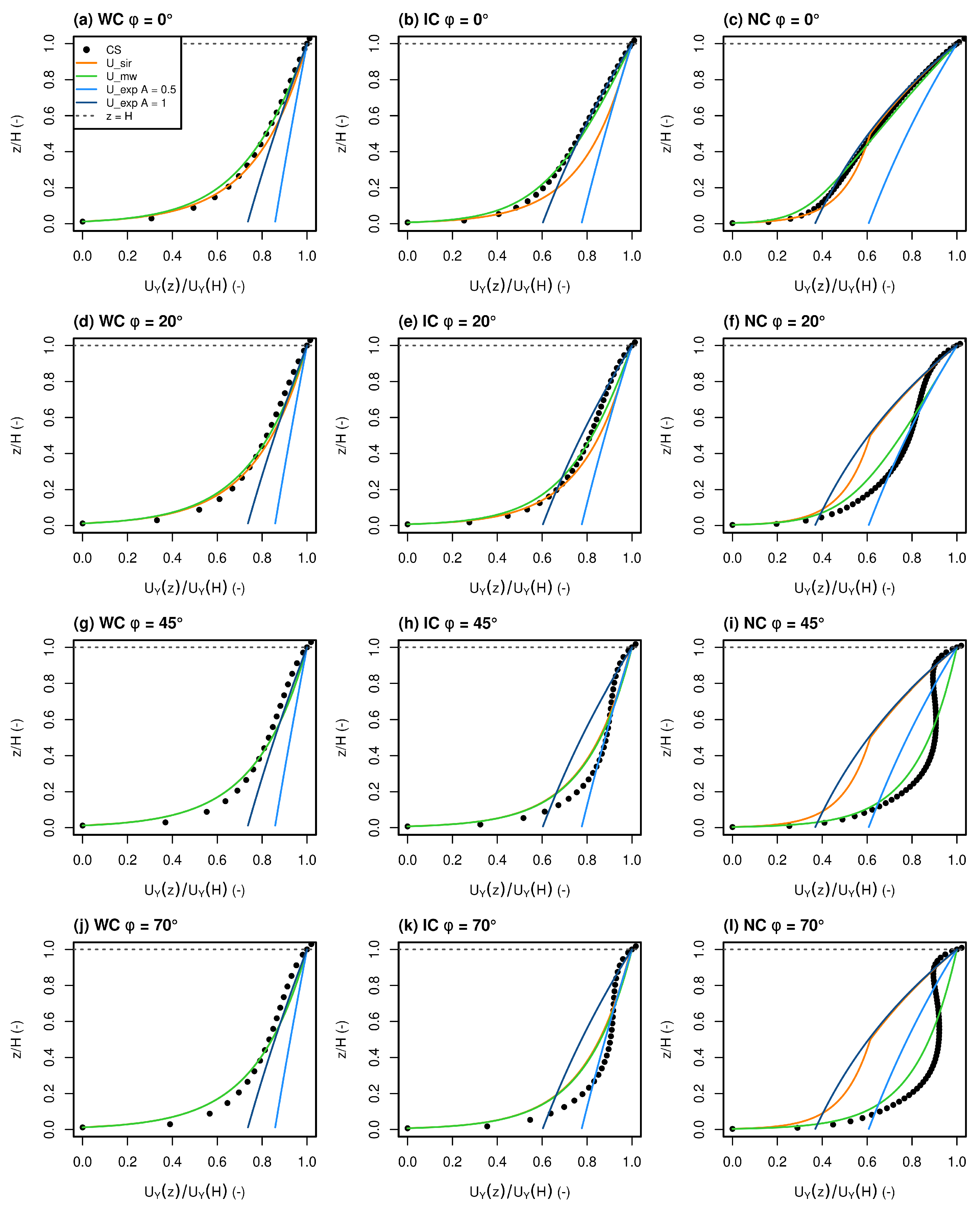
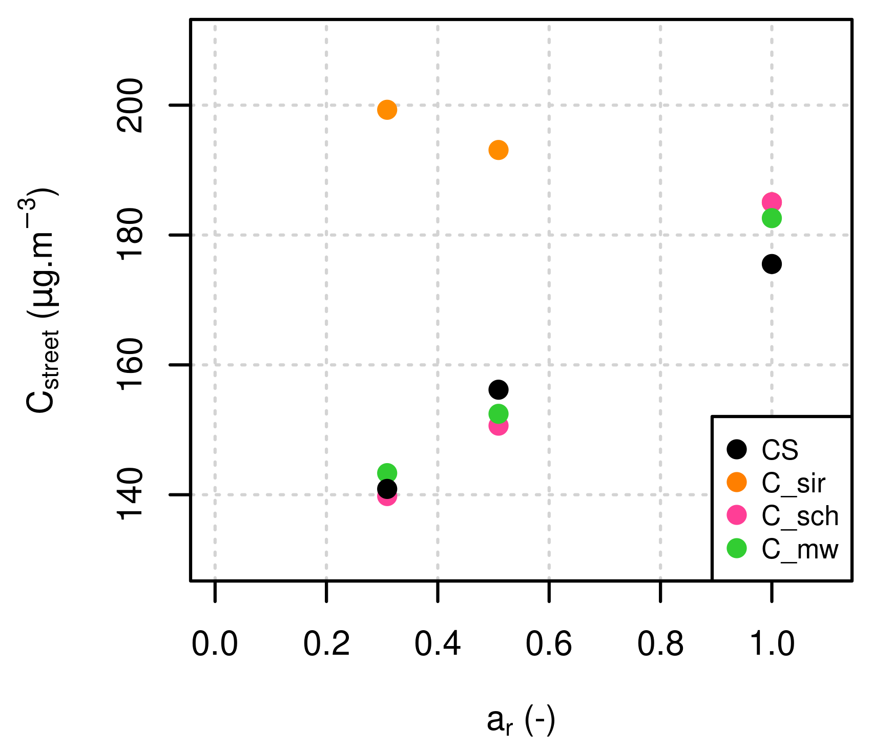
A parametrization that was originally developed for flow in sparse and dense vegetated canopies was adapted to represent the flow in street canyons in the Model of Urban Network of Intersecting Canyons and Highways (MUNICH) based on CFD simulations performed with the Code_Saturne code. The different MUNICH flow parametrizations and Code_Saturne simulations were compared by spatially averaging the wind speed and the passive tracer concentration in the street and the background domains.

The newly adapted parametrization is based on an analytical resolution of the momentum equation within sparse and dense vegetated canopies developed by Wang [37,38]. Assuming a homogeneous canopy, the vertical transfer coefficient profile is proportional to the distance from the ground and depends on the canopy features (the height and frontal area density). The vertical wind speed profile is also a function of the canopy features; this converges to a logarithmic profile in the no-canopy scenario and tends to an exponential profile when the frontal area density of obstacles increases.

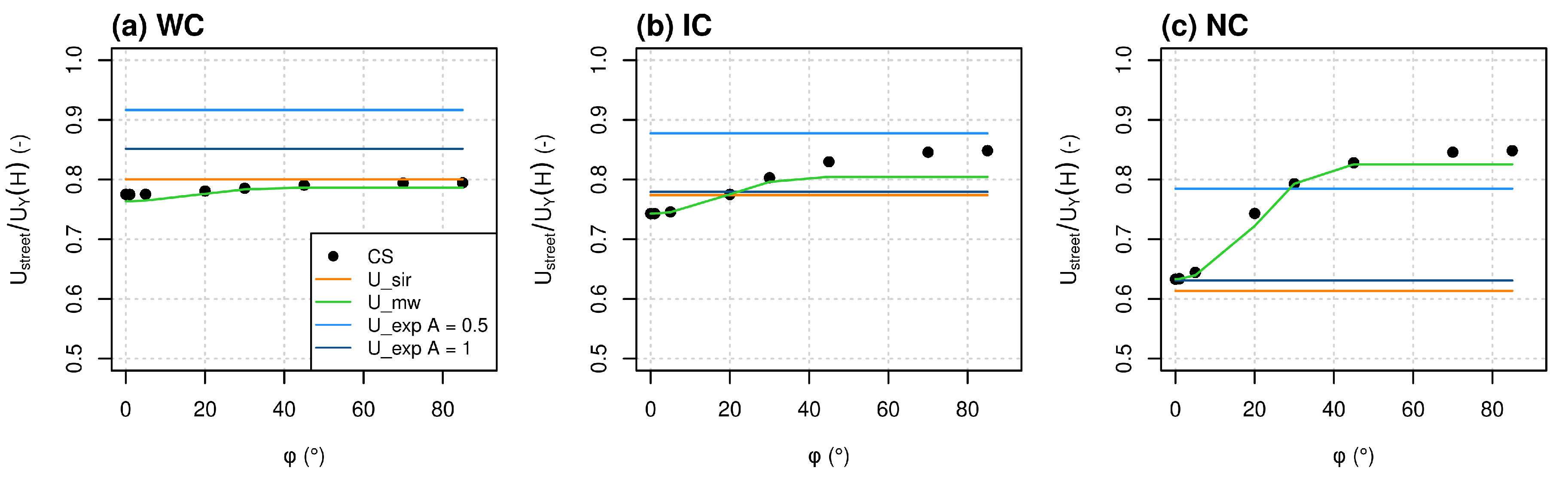
The Wang [37,38] equations were adapted to street canyons by modifying the value of two parameters, one involved in the characteristic length calculation and the other one in the wind speed attenuation coefficient. The street canyon aspect ratio was multiplied by a function of the wind angle to consider the variation of the wind speed in the street with this wind angle (only for horizontal transfers). The modified parameters were determined to maximize the agreement with Code_Saturne simulations: for the average wind speed in the street, the normalized mean absolute error ranged from 1.0% to 1.9%, and the normalized mean bias ranged from −1.0% to −1.9%. For the vertical transfer coefficient, the relative deviation ranged from −4.1% to 2.8%.

Compared to other MUNICH parametrizations, this work added a dependence on the wind angle for the horizontal wind speed in the street. The formulation of the wind speed and vertical transfer coefficient is general and valid for a wide range of street–canyon and wind characteristics. Furthermore, it is simple enough to be easily modified to take new features into account. For example, in further work, the tree effect on air flow in street canyons will be parametrized to consider both building and tree effects on the horizontal wind speed and vertical transfer coefficient. In addition, this parametrization developed for pollutant dispersion could also be used in urban climate models to compute heat and water vapor transfers.

References

1. Faiz, A. Automotive emissions in developing countries-relative implications for global warming, acidification and urban air quality. Transp. Res. Part A Policy Pract. 1993, 27, 167–186. [Google Scholar] [CrossRef]
2. Akimoto, H. Global Air Quality and Pollution. Science 2003, 302, 1716–1719. [Google Scholar] [CrossRef] [PubMed] [Green Version]
3. Yuan, C.; Ng, E.; Norford, L.K. Improving air quality in high-density cities by understanding the relationship between air pollutant dispersion and urban morphologies. Build. Environ. 2014, 71, 245–258. [Google Scholar] [CrossRef] [PubMed]
4. Zhang, Y.; Gu, Z.; Yu, C.W. Impact Factors on Airflow and Pollutant Dispersion in Urban Street Canyons and Comprehensive Simulations: A Review. Curr. Pollut. Rep. 2020, 6, 425–439. [Google Scholar] [CrossRef]
5. Angel, S.; Parent, J.; Civco, D.L.; Blei, A.; Potere, D. The dimensions of global urban expansion: Estimates and projections for all countries, 2000–2050. Prog. Plan. 2011, 75, 53–107. [Google Scholar] [CrossRef]
6. Pascal, M.; Corso, M.; Chanel, O.; Declercq, C.; Badaloni, C.; Cesaroni, G.; Henschel, S.; Meister, K.; Haluza, D.; Martin-Olmedo, P.; et al. Assessing the public health impacts of urban air pollution in 25 European cities: Results of the Aphekom project. Sci. Total Environ. 2013, 449, 390–400. [Google Scholar] [CrossRef]
7. West, J.J.; Cohen, A.; Dentener, F.; Brunekreef, B.; Zhu, T.; Armstrong, B.; Bell, M.L.; Brauer, M.; Carmichael, G.; Costa, D.L.; et al. What We Breathe Impacts Our Health: Improving Understanding of the Link between Air Pollution and Health. Environ. Sci. Technol. 2016, 50, 4895–4904. [Google Scholar] [CrossRef]
8. Borck, R.; Schrauth, P. Population density and urban air quality. Reg. Sci. Urban Econ. 2021, 86, 103596. [Google Scholar] [CrossRef]
9. Demetriou, E.; Hadjistassou, C. Lowering mortality risks in urban areas by containing atmospheric pollution. Environ. Res. 2022, 211, 113096. [Google Scholar] [CrossRef]
10. Harman, I.N.; Barlow, J.F.; Belcher, S.E. Scalar fluxes from urban street canyons. Part II Model. Bound.-Lay. Meteorol. 2004, 113, 387–409. [Google Scholar] [CrossRef]
11. Cai, X.M.; Barlow, J.F.; Belcher, S.E. Dispersion and transfer of passive scalars in and above street canyons—Large-eddy simulations. Atmos. Environ. 2008, 42, 5885–5895. [Google Scholar] [CrossRef]
12. Vardoulakis, S.; Fisher, B.E.; Pericleous, K.; Gonzalez-Flesca, N. Modelling air quality in street canyons: A review. Atmos. Environ. 2003, 37, 155–182. [Google Scholar] [CrossRef] [Green Version]
13. Huang, Y.D.; Hou, R.W.; Liu, Z.Y.; Song, Y.; Cui, P.Y.; Kim, C.N. Effects of Wind Direction on the Airflow and Pollutant Dispersion inside a Long Street Canyon. Aerosol Air Qual. Res. 2019, 19, 1152–1171. [Google Scholar] [CrossRef]
14. Zhang, K.; Chen, G.; Wang, X.; Liu, S.; Mak, C.M.; Fan, Y.; Hang, J. Numerical evaluations of urban design technique to reduce vehicular personal intake fraction in deep street canyons. Sci. Total Environ. 2019, 653, 968–994. [Google Scholar] [CrossRef] [PubMed]
15. Yang, H.; Chen, T.; Lin, Y.; Buccolieri, R.; Mattsson, M.; Zhang, M.; Hang, J.; Wang, Q. Integrated impacts of tree planting and street aspect ratios on CO dispersion and personal exposure in full-scale street canyons. Build. Environ. 2020, 169, 106529. [Google Scholar] [CrossRef]
16. Miao, C.; Yu, S.; Zhang, Y.; Hu, Y.; He, X.; Chen, W. Assessing outdoor air quality vertically in an urban street canyon and its response to microclimatic factors. J. Environ. Sci. 2022. [Google Scholar] [CrossRef]
17. Collett, R.S.; Oduyemi, K. Air quality modelling: A technical review of mathematical approaches. Meteorol. Appl. 1997, 4, 235–246. [Google Scholar] [CrossRef]
18. Zhang, Y.; Sartelet, K.; Wu, S.Y.; Seigneur, C. Application of WRF/Chem-MADRID and WRF/Polyphemus in Europe, Part I: Model description, evaluation of meteorological predictions, and aerosol-meteorology interactions. Atmos. Chem. Phys. 2013, 13, 6845–6875. [Google Scholar] [CrossRef] [Green Version]
19. Mailler, S.; Menut, L.; Khvorostyanov, D.; Valari, M.; Couvidat, F.; Siour, G.; Turquety, S.; Briant, R.; Tuccella, P.; Bessagnet, B.; et al. CHIMERE-2017: From urban to hemispheric chemistry-transport modeling. Geosci. Model Dev. 2017, 10, 2397–2423. [Google Scholar] [CrossRef] [Green Version]
20. Appel, K.W.; Napelenok, S.L.; Foley, K.M.; Pye, H.O.T.; Hogrefe, C.; Luecken, D.J.; Bash, J.O.; Roselle, S.J.; Pleim, J.E.; Foroutan, H.; et al. Description and evaluation of the Community Multiscale Air Quality (CMAQ) modeling system version 5.1. Geosci. Model Dev. 2017, 10, 1703–1732. [Google Scholar] [CrossRef] [Green Version]
21. Berkowicz, R. OSPM—A parameterised street pollution model. Environ. Monit. Assess. 2000, 65, 323–331. [Google Scholar] [CrossRef]
22. Soulhac, L.; Salizzoni, P.; Cierco, F.X.; Perkins, R. The model SIRANE for atmospheric urban pollutant dispersion; part I, presentation of the model. Atmos. Environ. 2011, 45, 7379–7395. [Google Scholar] [CrossRef]
23. Soulhac, L.; Nguyen, C.; Volta, P.; Salizzoni, P. The model SIRANE for atmospheric urban pollutant dispersion. PART III: Validation against NO2 yearly concentration measurements in a large urban agglomeration. Atmos. Environ. 2017, 167, 377–388. [Google Scholar] [CrossRef]
24. Kim, Y.; Wu, Y.; Seigneur, C.; Roustan, Y. Multi-scale modeling of urban air pollution: Development and application of a Street-in-Grid model (v1.0) by coupling MUNICH (v1.0) and Polair3D (v1.8.1). Geosci. Model Dev. 2018, 11, 611–629. [Google Scholar] [CrossRef] [Green Version]
25. Lugon, L.; Sartelet, K.; Kim, Y.; Vigneron, J.; Chrétien, O. Nonstationary modeling of NO2, NO and NOx in Paris using the Street-in-Grid model: Coupling local and regional scales with a two-way dynamic approach. Atmos. Chem. Phys. 2020, 20, 7717–7740. [Google Scholar] [CrossRef]
26. Lugon, L.; Sartelet, K.; Kim, Y.; Vigneron, J.; Chrétien, O. Simulation of primary and secondary particles in the streets of Paris using MUNICH. Faraday Discuss. 2021, 226, 432–456. [Google Scholar] [CrossRef]
27. Li, X.; Liu, C.; Leung, D.; Lam, K. Recent progress in CFD modelling of wind field and pollutant transport in street canyons. Atmos. Environ. 2006, 40, 5640–5658. [Google Scholar] [CrossRef]
28. Tominaga, Y.; Stathopoulos, T. CFD simulation of near-field pollutant dispersion in the urban environment: A review of current modeling techniques. Atmos. Environ. 2013, 79, 716–730. [Google Scholar] [CrossRef] [Green Version]
29. Salim, S.M.; Buccolieri, R.; Chan, A.; Di Sabatino, S. Numerical simulation of atmospheric pollutant dispersion in an urban street canyon: Comparison between RANS and LES. J. Wind Eng. Ind. Aerod. 2011, 99, 103–113. [Google Scholar] [CrossRef]
30. Aliabadi, A.A.; Moradi, M.; Byerlay, R.A.E. The budgets of turbulence kinetic energy and heat in the urban roughness sublayer. Environ. Fluid Mech. 2021, 21, 843–884. [Google Scholar] [CrossRef]
31. Sartelet, K.; Zhu, S.; Moukhtar, S.; André, M.; André, J.M.; Gros, V.; Favez, O.; Brasseur, A.; Redaelli, M. Emission of intermediate, semi and low volatile organic compounds from traffic and their impact on secondary organic aerosol concentrations over Greater Paris. Atmos. Environ. 2018, 180, 126–137. [Google Scholar] [CrossRef]
32. Archambeau, F.; Méchitoua, N.; Sakiz, M. Code Saturne: A finite volume code for the computation of turbulent incompressible flows-Industrial applications. Int. J. Finite Vol. 2004, 1, 1–62. [Google Scholar]
33. Milliez, M.; Carissimo, B. Numerical simulations of pollutant dispersion in an idealized urban area, for different meteorological conditions. Bound.-Lay. Meteorol. 2007, 122, 321–342. [Google Scholar] [CrossRef]
34. Milliez, M.; Carissimo, B. Computational Fluid Dynamical Modelling of Concentration Fluctuations in an Idealized Urban Area. Bound.-Lay. Meteorol. 2008, 127, 241–259. [Google Scholar] [CrossRef]
35. Gao, Z.; Bresson, R.; Qu, Y.; Milliez, M.; de Munck, C.; Carissimo, B. High resolution unsteady RANS simulation of wind, thermal effects and pollution dispersion for studying urban renewal scenarios in a neighborhood of Toulouse. Urban Clim. 2018, 23, 114–130. [Google Scholar] [CrossRef]
36. Zaïdi, H.; Dupont, E.; Milliez, M.; Musson-Genon, L.; Carissimo, B. Numerical Simulations of the Microscale Heterogeneities of Turbulence Observed on a Complex Site. Bound.-Lay. Meteorol. 2013, 147, 237–259. [Google Scholar] [CrossRef]
37. Wang, W. An Analytical Model for Mean Wind Profiles in Sparse Canopies. Bound.-Lay. Meteorol. 2012, 142, 383–399. [Google Scholar] [CrossRef]
38. Wang, W. Analytically Modelling Mean Wind and Stress Profiles in Canopies. Bound.-Lay. Meteorol. 2014, 151, 239–256. [Google Scholar] [CrossRef]
39. Schulte, N.; Tan, S.; Venkatram, A. The ratio of effective building height to street width governs dispersion of local vehicle emissions. Atmos. Environ. 2015, 112, 54–63. [Google Scholar] [CrossRef]
40. Salizzoni, P.; Soulhac, L.; Mejean, P. Street canyon ventilation and atmospheric turbulence. Atmos. Environ. 2009, 43, 5056–5067. [Google Scholar] [CrossRef]
41. Wang, Y.; Sartelet, K.; Bocquet, M.; Chazette, P. Modelling and assimilation of lidar signals over Greater Paris during the MEGAPOLI summer campaign. Atmos. Chem. Phys. 2014, 3511–3532. [Google Scholar] [CrossRef] [Green Version]
42. Kim, Y.; Sartelet, K.; Raut, J.C.; Chazette, P. Influence of an urban canopy model and PBL schemes on vertical mixing for air quality modeling over Greater Paris. Atmos. Environ. 2015, 107, 289–306. [Google Scholar] [CrossRef] [Green Version]
43. Masson, V. A Physically-Based Scheme For The Urban Energy Budget In Atmospheric Models. Bound.-Lay. Meteorol. 2000, 94, 357–397. [Google Scholar] [CrossRef]
44. Lemonsu, A.; Grimmond, C.S.B.; Masson, V. Modeling the Surface Energy Balance of the Core of an Old Mediterranean City: Marseille. J. Appl. Meteorol. 2004, 43, 312–327. [Google Scholar] [CrossRef]
45. Cherin, N.; Roustan, Y.; Musson-Genon, L.; Seigneur, C. Modelling atmospheric dry deposition in urban areas using an urban canopy approach. Geosci. Model Dev. 2015, 8, 893–910. [Google Scholar] [CrossRef] [Green Version]
46. Macdonald, R.W.; Griffiths, R.F.; Hall, D.J. An improved method for the estimation of surface roughness of obstacle arrays. Atmos. Environ. 1998, 32, 1857–1864. [Google Scholar] [CrossRef]
47. Grimmond, C.S.B.; Oke, T.R. Aerodynamic Properties of Urban Areas Derived from Analysis of Surface Form. J. Appl. Meteorol. 1999, 38, 1262–1292. [Google Scholar] [CrossRef]
48. Soulhac, L.; Perkins, R.J.; Salizzoni, P. Flow in a Street Canyon for any External Wind Direction. Bound.-Lay. Meteorol. 2008, 126, 365–388. [Google Scholar] [CrossRef]
49. Castro, I.P. Are Urban-Canopy Velocity Profiles Exponential? Bound.-Lay. Meteorol. 2017, 164, 337–351. [Google Scholar] [CrossRef]
50. Katul, G.G.; Mahrt, L.; Poggi, D.; Sanz, C. ONE- and TWO-Equation Models for Canopy Turbulence. Bound.-Lay. Meteorol. 2004, 113, 81–109. [Google Scholar] [CrossRef] [Green Version]
51. Guimet, V.; Laurence, D. A linearised turbulent production in the k-ε model for engineering applications. In Engineering Turbulence Modelling and Experiments 5; Rodi, W., Fueyo, N., Eds.; Elsevier Science Ltd.: Oxford, UK, 2002; pp. 157–166. [Google Scholar] [CrossRef]
52. Richards, P.J.; Hoxey, R.P. Appropriate boundary conditions for computational wind engineering models using the k-ε turbulence model. J. Wind. Eng. Ind. Aerodyn. 1993, 46–47, 145–153. [Google Scholar] [CrossRef]
53. Wiernga, J. Representative roughness parameters for homogeneous terrain. Bound.-Lay. Meteorol. 1993, 63, 323–364. [Google Scholar] [CrossRef]
54. An, K.; Fung, J.C.H.; Yim, S.H.L. Sensitivity of inflow boundary conditions on downstream wind and turbulence profiles through building obstacles using a CFD approach. J. Wind Eng. Ind. Aerod. 2013, 115, 137–149. [Google Scholar] [CrossRef]
55. Oke, T.R. Boundary Layer Climates (Chapter 8, pp. 262–303), 2nd ed.; Routledge; Methuen: New York, NY, USA, 1987; p. 435. [Google Scholar]
Figure 1. 2D scheme of the canyon geometry with the street and background domain borders, and the boundary conditions.
Atmosphere 13 00527 g001
Figure 2. Comparison of the normalized vertical transfer coefficient ( q v e r t / ( u * H ) ) between Code_Saturne (CS), Soulhac et al. [22] (L_sir), Schulte et al. [39] (L_sch) and modified Wang [37] (L_mw) depending on a r .
Atmosphere 13 00527 g002
Figure 3. Comparison of the Code_Saturne vertical profile of wind speed in the street direction ( U Y ( z ) ) normalized by the wind speed at the roof level ( U H , φ ) for different wind angle ( φ ) and for (a) WC, (b) IC and (c) NC. (d) Comparison of the Code_Saturne average wind speed in the street ( U s t r e e t ) normalized by U H , φ depending on φ and for the three canyons.
Atmosphere 13 00527 g003
Figure 4. Comparison of the wind speed attenuation coefficient ( α ) between Code_Saturne and the modified Wang [37,38] parametrization (U_mw) (a) depending on φ and (b) canyon aspect ratio ( a r ) in the φ = 0 case for the three canyons.
Atmosphere 13 00527 g004
Figure 5. Comparison of U s t r e e t normalized by U H , φ between Code_Saturne and the different MUNICH parametrizations for (a) WC, (b) IC and (c) NC and depending on φ .
Atmosphere 13 00527 g005
Figure 6. Comparison of U Y ( z ) normalized by U H , φ between Code_Saturne and the different MUNICH parametrizations for (a,d,g,j) WC, (b,e,h,k) IC, (c,f,i,l) NC and for (ac) φ = 0 , (df) φ = 20 , (gi) φ = 45 and (j,k,l) φ = 70 .
Atmosphere 13 00527 g006