Article

Wind Speed Statistics from a Small UAS and Its Sensitivity to Sensor Location

School of Mechanical & Aerospace Engineering, Oklahoma State University, Stillwater, OK 74078, USA
*
Author to whom correspondence should be addressed.
Atmosphere 2022, 13(3), 443; https://doi.org/10.3390/atmos13030443
Submission received: 31 December 2021 / Revised: 4 March 2022 / Accepted: 6 March 2022 / Published: 9 March 2022
(This article belongs to the Special Issue Transport Phenomena in the Atmospheric Boundary Layer)

Abstract

:
With the increase in the use of small uncrewed aircraft systems (UAS) there is a growing need for real-time weather forecasting to improve the safety of low-altitude aircraft operations. This will require integration of measurements with autonomous systems since current available sampling lack sufficient resolution within the atmospheric boundary layer (ABL). Thus, the current work aims to assess the ability to measure wind speeds from a quad-copter UAS and compare the performance with that of a fixed mast. Two laboratory tests were initially performed to assess the spatial variation in the vertically induced flow from the rotors. The horizontal distribution above the rotors was examined in a water tunnel at speeds and rotation rates to simulate nominally full throttle with a relative air speed of 0 or 8 m/s. These results showed that the sensor should be placed between rotor pairs. The vertical distribution was examined from a single rotor test in a large chamber, which suggested that at full throttle the sensor should be about 400 mm above the rotor plane. Field testing was then performed with the sensor positioned in between both pairs of rotors at 406, 508, and 610 mm above the rotor plane. The mean velocity over the given period was within 5.5% of the that measured from a fixed mast over the same period. The variation between the UAS and mast sensors were better correlated with the local mean shear than separation distance, which suggests height mismatch could be the source of error. The fluctuating velocity was quantified with the comparison of higher order statistics as well as the power spectral density, which the mast and UAS spectra were in good agreement regardless of the separation distance. This implies that for the current configuration a separation distance of 5.3 rotor diameters was sufficient to minimize the influence of the rotors.

1. Introduction

As the amount of small uncrewed aircraft systems (UAS) increases, better real-time weather forecasting in the lower atmosphere is needed. One way to improve these forecasts is to acquire accurate in situ data with high spatiotemporal resolution. This is what a UAS excels at, and these more accurate forecasts can be used in real-time weather prediction to aid in improving the safety and efficiency of low-altitude aircraft operations. The first in situ measurements of the atmosphere were made using towers (or masts) and ground based measurements of wind speed, wind direction, and temperature. However, a tower can only sample within the surface layer of the atmosphere and has limited ability to provide spatial information (i.e., only can get the local vertical wind shear). The next progression was to use weather balloons, which work extremely well at acquiring vertical profiles of the atmosphere, typically using radiosondes. Balloon-based radiosonde measurements have been performed daily or twice-daily at stations across the globe since the 1940s [1]. A limitation of these measurements is that they rapidly ascend (especially through the atmospheric boundary layer), provide only a single measurement for a given altitude, and lack the ability to control the position of the measurement. A method used to bypass this limitation is the use of tethered balloons. These tethers allow for controlled height and the ability to go up and down multiple times [2,3,4]. UAS-based atmospheric profiles provide a complimentary alternative to these traditional approaches to make direct point measurements. Recently there has been significant work demonstrating the ability to acquire accurate atmospheric measurements from UAS [5,6,7,8,9,10,11,12,13,14]. UAS are broadly divided into two categories, fixed wing and multi-rotor. Fixed wing UAS allow for long duration flights that enable sampling over large areas, but the UAS dynamics limits its mobility and requires larger unobstructed space [15]. However, multi-rotor UAS, like the example shown in Figure 1, excel in the areas where the fixed wings are limited. Particularly due to their ability to hover.
While fixed wing UAS measurements can locate sensors ahead of the leading edge to ensure the measurements are within “clean air”, it is more difficult for multi-rotor systems to separate the atmospheric measurement from the interaction of the rotors. This interaction comes from several mechanisms including rotor outflow (down-wash), in-plane flow, and inflow depending on the location of the sensors and the orientation relative to the flight direction. An investigation of the down-wash was performed by Whyte et al. [16] and indicated that the induced velocity is higher in the outflow region. This indicates that positioning a sensor in or near the down-wash is not optimal. Similarly, positioning sensors inline with the rotors has proven to be sub-optimal as there are large amounts of turbulence in this region. The turbulence is created by the interaction between the tip vortices with each other as well as the body of the UAS [17].
Initial investigations [18,19] indicate that sensor placement in the inflow region (i.e., above the rotors) is the preferred location. Thus, the focus of the current study is on quantifying the rotor induced velocity in the inflow region and then field testing with the sensor positioned as identified in the laboratory tests. The field test measurements are compared against similar measurements from a nearby fixed mast. However, it should also be noted that there are promising new measurement developments in the area of UAS based lidar that would be less sensitive to the previously discussed conditions [20,21]. The remainder of the paper presents the experimental methods in Section 2, results of the various experiments in Section 3, a discussion focused on comparing quad-rotor UAS velocity measurements to mast-based measurements in Section 4, and finally conclusions in Section 5. The results section is divided into two parts, laboratory testing and field testing. The laboratory testing summarizes a series of tests with a variety of configurations where the resulting in-flow velocity field were measured [22]. The conclusions from the laboratory tests were used to position the sensor during the field testing, which explored a subset of sensor positions within the inflow while simultaneously acquiring similar measurements from a nearby mast.

2. Materials and Methods

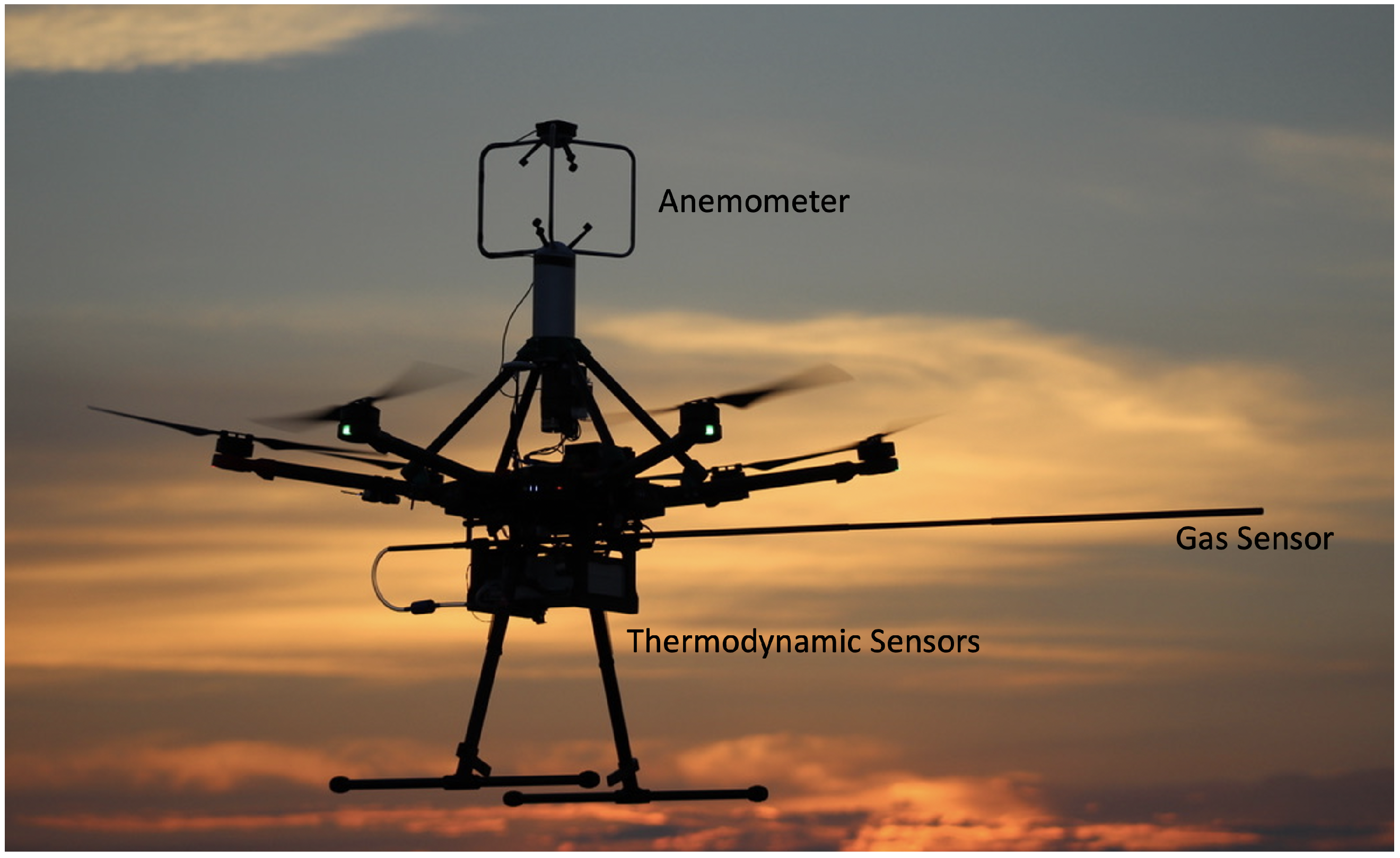
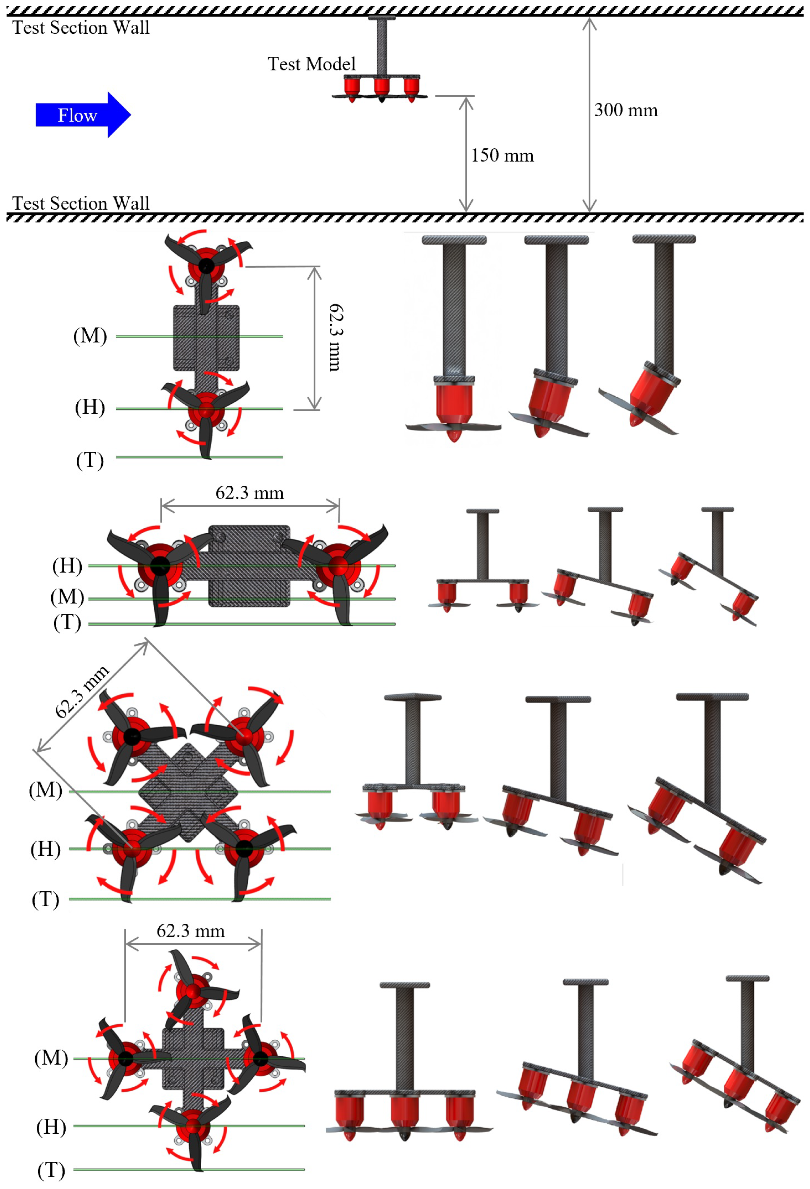
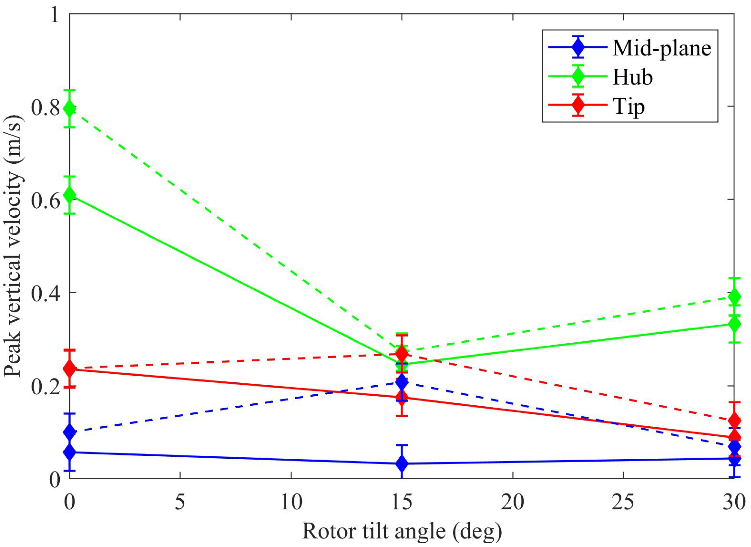
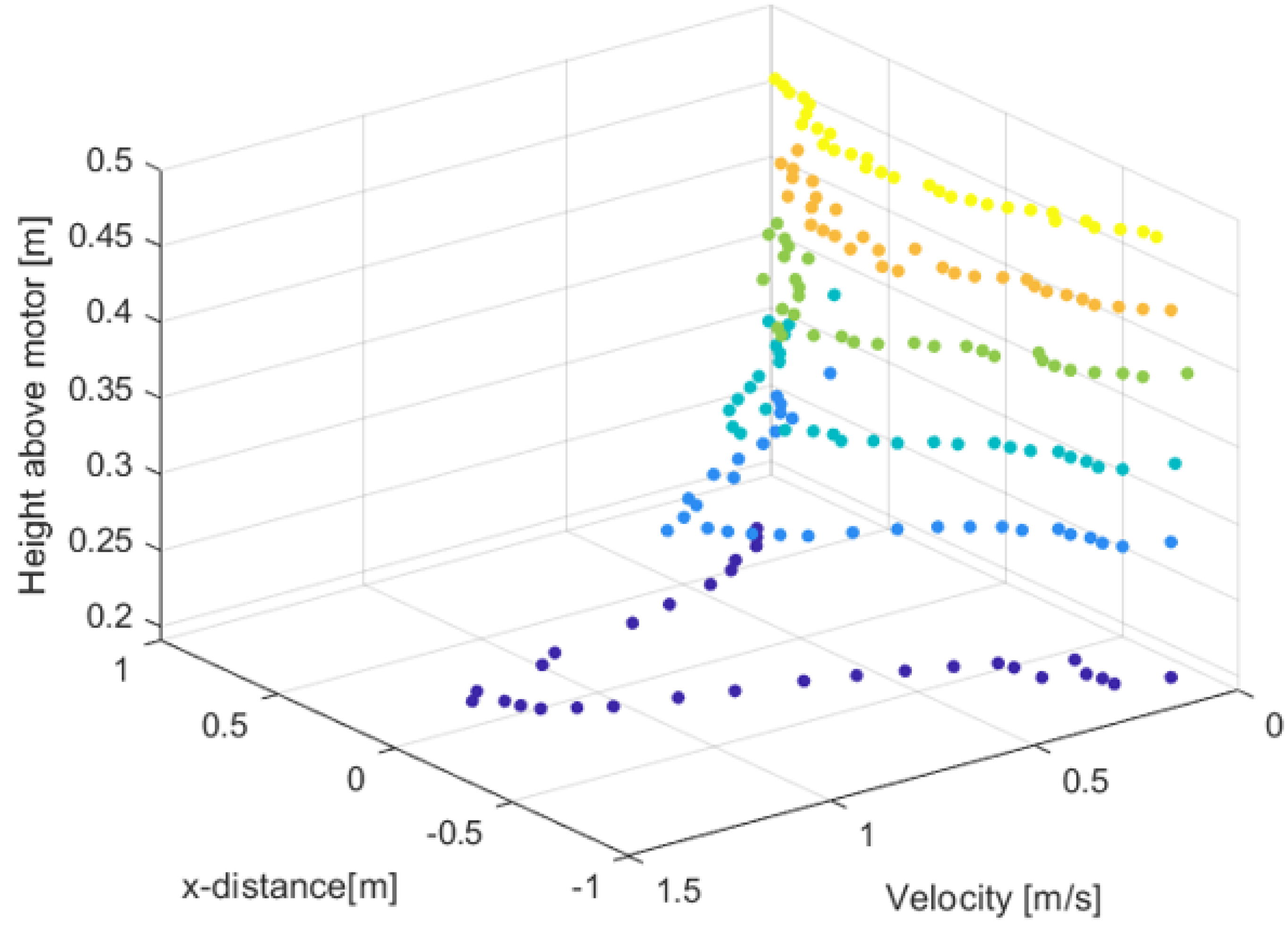
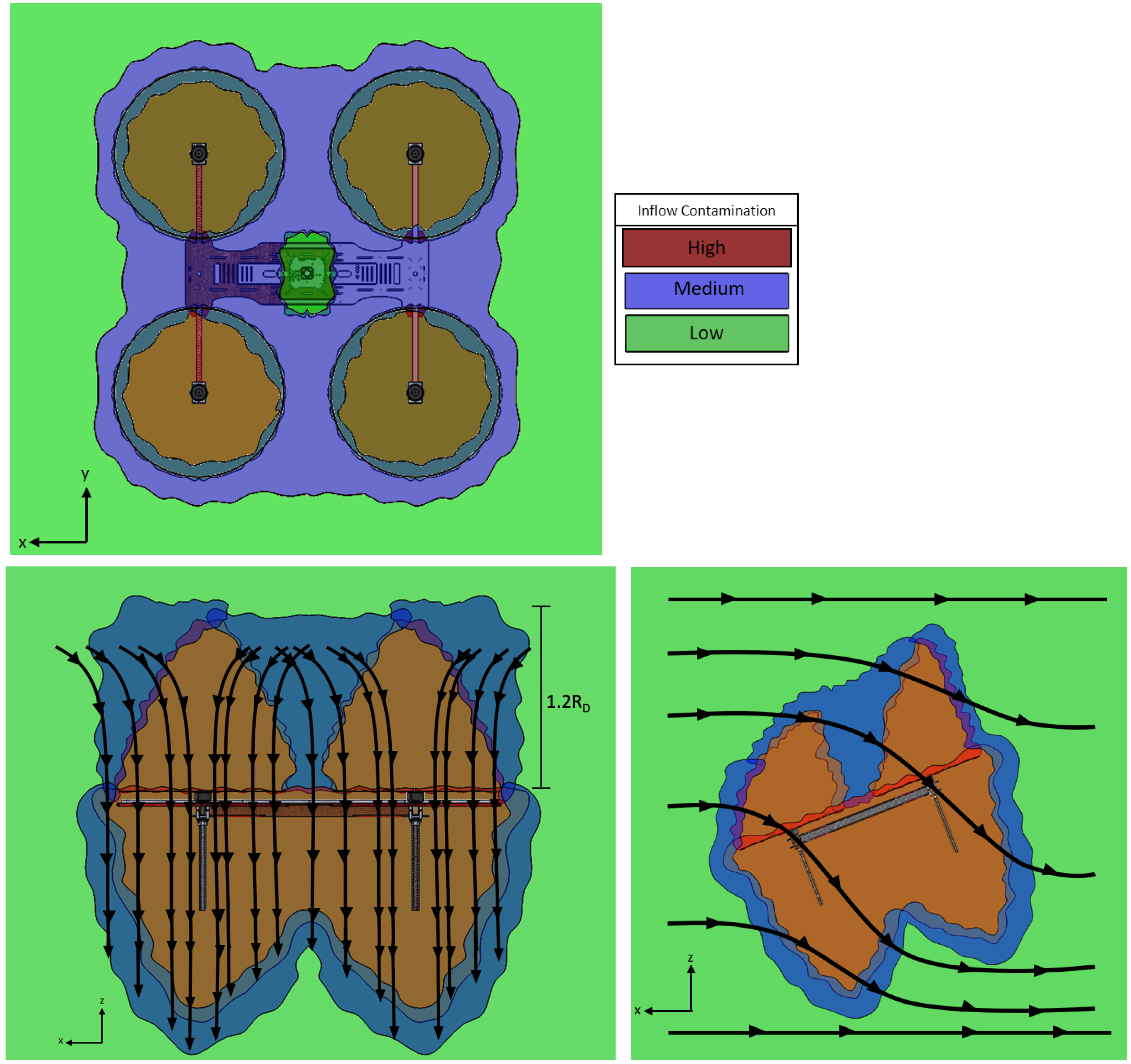
2.1. Laboratory Testing
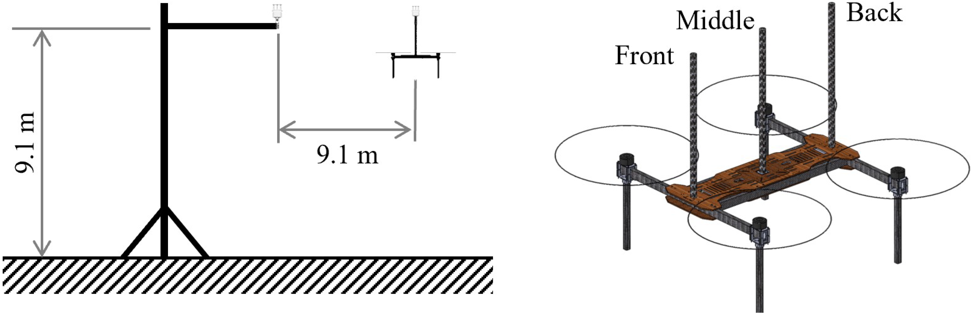
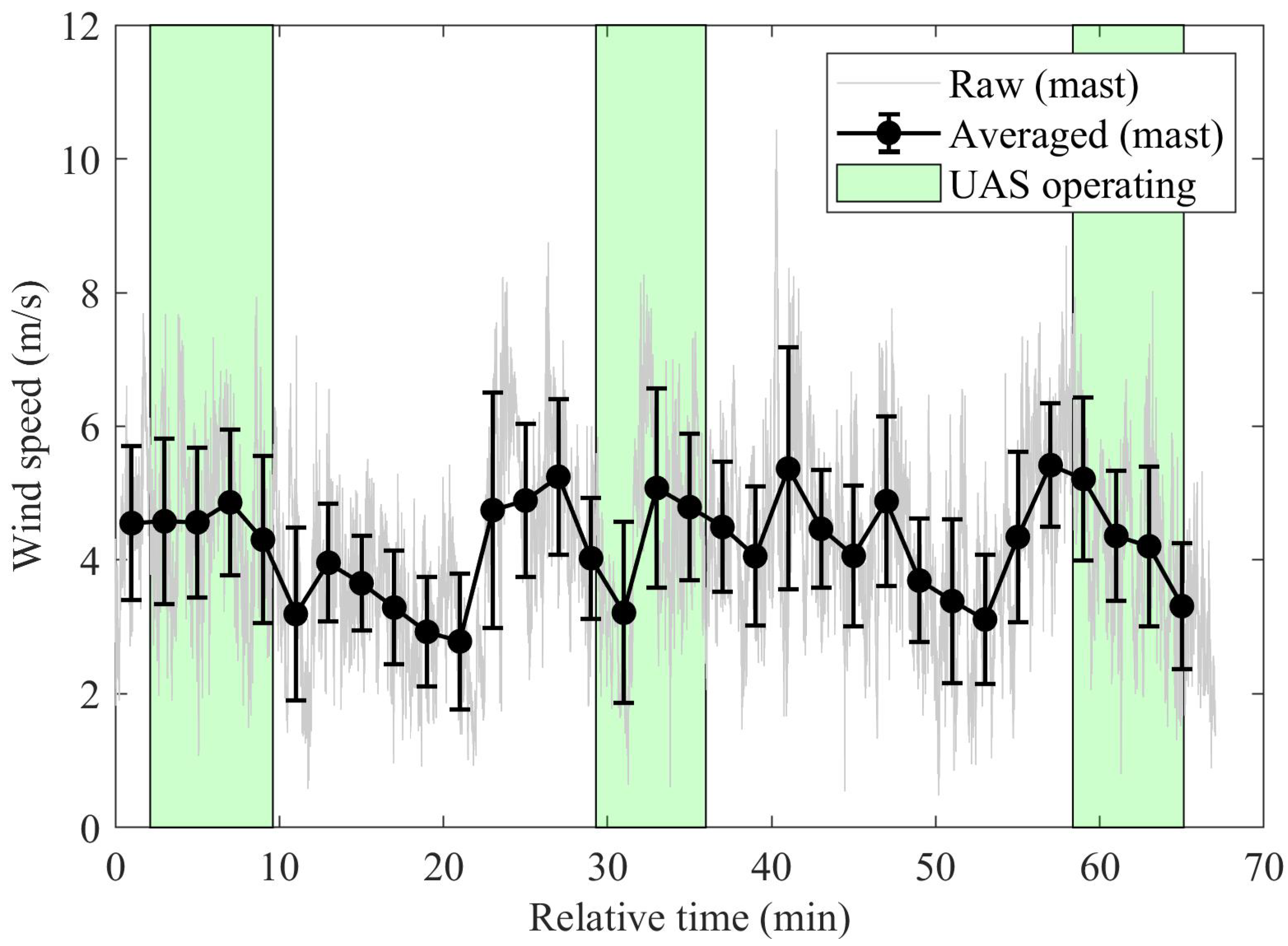
A detailed investigation of the flow-field induced by the multi-rotor system was performed using particle image velocimetry (PIV) in the flow visualization water tunnel (Model 503, Engineering Lab Design, Lake City, MN, USA) at Oklahoma State University (Stillwater, OK, USA). The tests were performed by submerging a custom rotor system into the water tunnel test section. The test section had a cross-sectional area of 300 mm by 300 mm and a length of 1 m. The minimum and maximum operating speeds were 9 mm/s and 1100 mm/s, respectively, which was achieved with two centrifugal pumps that were independently controlled with variable frequency drives. Additional water tunnel details are provided in Lucido et al. [23].
There were four primary rotor configurations (see Figure 2) tested, (i) dual-rotor perpendicular, (ii) dual-rotor parallel, (iii) quad-rotor plus-configuration, and (iv) quad-rotor cross-configuration. Each rotor configuration was selected to observe specific characteristics of multi-rotor systems. Dual-rotor perpendicular has the two rotors positioned at single stream-wise location in the test section and spanning the center portion of the cross-section. This configuration allows the flow to be examined for a single rotor. Dual-rotor parallel has the two rotors centered in the tunnel span and positioned at different downstream locations, which allows the interactions between two rotors to be examined. The quad-rotor configurations were selected since they are the most popular quad-copter systems. The plus-configuration has a single rotor lead the aircraft [24] with a second rotor directly downstream of the leading rotor while the other two are centered between the first two in the dual-rotor perpendicular configuration. Since the quad-rotor configuration is symmetric about 90 degree rotations, the cross-configuration [24] is a 45 degree rotation from the plus-configuration (i.e., two of the rotors now lead the aircraft). A given rotor configuration was installed by mounting the motors upside down within the test section and feeding the wires through the top wall. The wiring, power, and control of the rotors is discussed in detail in Brenner [22]. The rotors (3052, GemFan, Ningbo, China) were 3-bladed with 76.2 mm (3-inch) diameters. Other blade sizes were tested but these were the only ones with sufficient strength to withstand the loading in the water tunnel.
The rotor inflow velocity field was measured with 2D-PIV with the image plane aligned in the streamwise direction. The nominal field-of-view was 300 mm × 290 mm, but the measurement region was limited to a smaller circular region due to significant vignetting. The inflow image plane was illuminated with a pair of Nd:YAG pulsed lasers (Ultra 50, Big Sky Laser Technologies, Bozeman, MT, USA) with a 532 nm wavelength. The scattered light from the image plane was captured with a high-speed camera (Motion Pro X3, Redlake, Woodsville, NH, USA) with a 1280 × 1240 pixel resolution. For each test condition, 500 images were acquired with a 1000 microsecond exposure. Since the various rotor configurations are inherently three dimensional, for each configuration there were three separate laser planes nominally corresponding to locations at the tip, hub, and mid-planes as illustrated in Figure 2. Note that the laser positions are only on one side of a given test configuration, which was to minimize test conditions given that the test configurations were symmetrical about their centerlines. The vector fields were computed using a commercial software package (DaVis 8.2.1, LaVision, Ypsilanti, MI, USA) and masking the rotors. Standard multi-pass cross-correlation with decreasing interrogation window size was used to compute the vector fields. The average vector fields were then exported for further analysis. The uncertainty was calculated to be approximately 3% due to limitations of the PIV processing algorithms and noise. Additional details are provided in Brenner [22].
The projected area of the models varied with configuration and tilt angle producing ratios of solid blockage area to total area ranging from 3.4% (dual parallel at 0° tilt angle) to 9.6% (quad-plus at 30° tilt angle). This range of blockage is comparable to traditional helicopter hub water tunnel experiments with values above 8% [25,26], which those studies reported negligible impact from blockage on the results. Correcting the freestream speed for the solid blockage increases the Reynolds number and advance ratio for the 0.5 m/s condition by less than 7%. More significantly, the current study focuses on vertical induced motions, which the experimental configuration only had 2 rotor diameters separation between the model and the bottom tunnel wall. Consequently, the PIV results focus on horizontal spatial variation and a separate laboratory test was performed to quantify vertical variation.
Testing was performed with the water tunnel inlet speed at 0 m/s (hovering condition) or 0.5 m/s. Correcting for the solid blockage effects, the freestream speed increased from 0.5 m/s at the inlet to between 0.52 m/s (dual parallel at 0° tilt angle) and 0.55 m/s (quad-plus at 30° tilt angle) at the model. The rotor diameter based Reynolds number ( R e = U D / ν ) and advance ratio ( μ = 2 U / ω D ) had ranges of 39,400 to 42,200 and 0.144 to 0.154, respectively. Here D is the rotor diameter (76.2 mm), U is the freestream speed at the model (corrected for blockage), ν is the kinematic viscosity ( 10 6 m 2 / s for water), and ω is the angular rotation speed of the blades. The PIV testing held the angular speed constant at 15 Hz ( ω = 94.2 rad/s). Note that assuming the model was full scale, the corresponding relative air speed for a nominal viscosity of 1.5 × 10 5 m 2 / s would be between 7.8 and 8.3 m/s, which is within the typical operation range. Similarly, the 900 RPM corresponds to a full scale rotor speed in air of 225 Hz, which is comparable to the upper end of a UAS at full throttle. Thus, the Reynolds number and advance ratio varied by less than 7% over all test conditions examined with PIV and these values are comparable to typical UAS flight conditions.
A second laboratory test examined the vertical variation in the inflow above a single rotor within static ambient conditions with the goal of getting a nominal measure of how far above the rotor is required to mitigate the influence of the rotor inflow prior to field testing. The inflow above a single m600 rotor was measured with an ultrasonic anemometer (FT205, FT Technologies, Sunbury-on-Thames, UK). The anemometer was mounted on a 27 mm diameter strut (following the manufacturer recommendations) that was attached to a movable boom arm that could vary the vertical position of the sensor from 200 to 480 mm above the rotor. Note that the strut was in the same horizontal plane as the boom such that the traversing boom was not above the rotor. The rotor was mounted on a single DJI m600 arm within a high ceiling chamber and operated at 1300 pwm. The rotor system consisted of DJI’s 2170 carbon fiber folding propeller, 2200 mah 3c lithium polymer (LiPo) battery, and a servo tester. Measurements of the flow field were taken by acquiring horizontal profiles above the rotor. This was done by traversing the rotor horizontally for each vertical position of the boom. The rotor was traversed a total of 2 m horizontally (1 m in each direction) to generate velocity profiles.

2.2. Field Testing

Field testing was performed with a heavy lift quad-copter UAS hovering 9.1 m above the ground and 9.1 m horizontally separated in the cross-wind direction from a fixed mast as illustrated in Figure 3 (left). The wind direction during these tests was coming from the north. Therefore, the UAS was flown to the west and slightly upstream (northward) of the mast’s position. This positioning was done to prevent wake effects from the mast on the drone. The deployable mast (BlueSky Mast, Largo, FL, USA) had an ultrasonic anemometer (ResponseONE 92000, Young, Traverse City, MI, USA) attached that could measure wind speed and direction at speeds up to 70 m/s. The sensor was mounted on a boom that was approximately 1 m long, to offset it from the center of the mast. This anemometer had an uncertainty of ± 0.3 m/s for speeds below 30 m/s, which the current study measured speeds below 10 m/s. This sensor is also capable of measuring atmospheric pressure, humidity, and temperature. The quad-copter UAS had a ultrasonic anemometer (Trisonica Mini Wind, Anemoment, Longmont, CO, USA) mounted above the rotors. The UAS anemometer was selected because it was lightweight (50 g) and had a similar resolution to that used on the mast (Model 92000, Young). The UAS anemometer can measure two-components of wind speed up to 50 m/s at a maximum rate of 4 Hz as well as measure temperature and relative humidity. The UAS anemometer could be mounted along the UAS centerline in the front, middle, or back (see Figure 3) at a height (H) above the rotors of 406, 508, or 610 mm. The current study only focused on measurements from the middle position as recommended from the results of the laboratory testing, but Brenner [22] provides results from all positions.
The UAS (SKB-1000, USRI, Stillwater, OK, USA) was a custom built electric powered quad-copter in the H-configuration. It was fabricated from carbon fiber and plywood and designed to carry heavy sensitive payloads. It was selected for this experiment due to its lift capabilities and its ease of mounting and integrating sensors. The payload consisted of the anemometer, a LiPo battery, data acquisition, and a flight controller (Pixhawk, Auterion, Zurich Switzerland) to get a GPS time stamp. The data acquisition system consisted of development board (Teensy, Arduino, Somerville, MA, USA) that logged the UAS anemometer signal and stored it on a micro SD card. The UAS anemometer was mounted on a 2-axis gimbal that was mounted on the top of the UAS platform. The gimbal was composed of two 9g servo motors that were controlled with an autopilot (Pixhawk Orange Cube, Hex Technology, Austin, TX, USA) using a “camera gimbal” mission planner plugin. The gimbal balances the UAS movement to keep the sensor level during flight. The UAS was flown such that the anemometer was at the same height as the mast anemometer. While the autopilot could precisely hold the UAS at a fixed height above the ground, the setting of the height to match that of the mast was done by manual inspection of the operator. The resulting height difference between the mast and UAS sensor was estimated to be approximately 0.3 m.
There were several other sources of uncertainty for this experiment that should be mentioned. First, the sensors were not identical, though comparable. Since the sensors were different between the mast and the UAS, two fixed ground tests were performed with both sensors next to each other. The mast sensor (92000, Young) was mounted on a tripod at the same height as the UAS sensor (Trisonica Mini), which had the UAS on the ground in the same configuration as it was flown. The difference in the means during each 5 min test window was approximately 0.06 m/s even though the second test was more than double the wind speed. The standard deviation was 10% to 13% higher with the UAS sensor (Trisonica Mini). These results show a nominal bias error between the sensors of 0.06 m/s with the UAS sensor being slightly noisier. Second, the two-axis gimbal system used to balance the UAS mounted sensor could introduce errors in the recorded data, which is especially true during sudden gusts of wind. There were also concerns about the operation conditions during testing including concerns about how rigid the mast anemometer was fixed to the mast, the UAS had unavoidable drift of about 0.1 m in position during a measurement period due to control limitations, and the natural variability of the surface layer combined with the inability to co-locate the two sensors.

3. Results

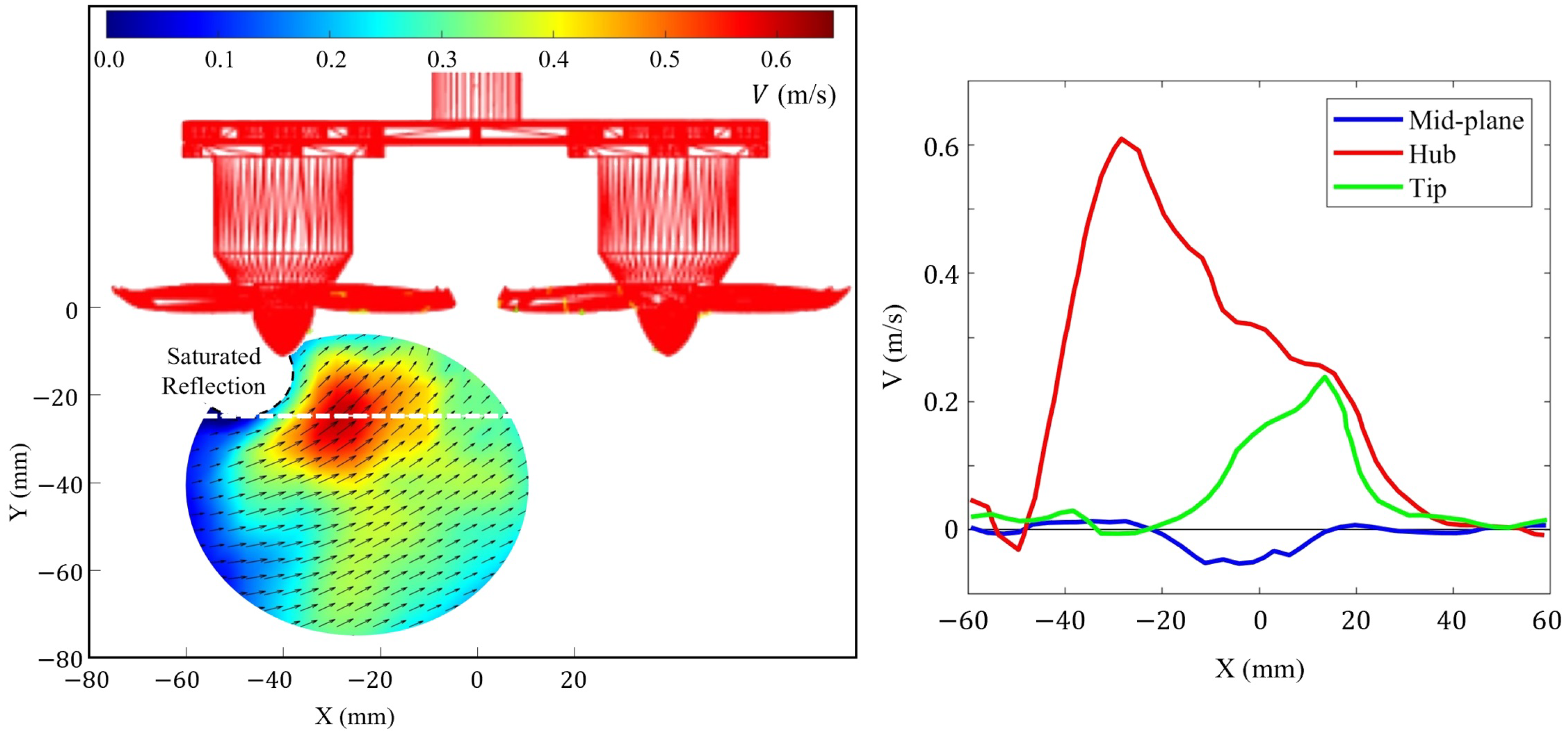
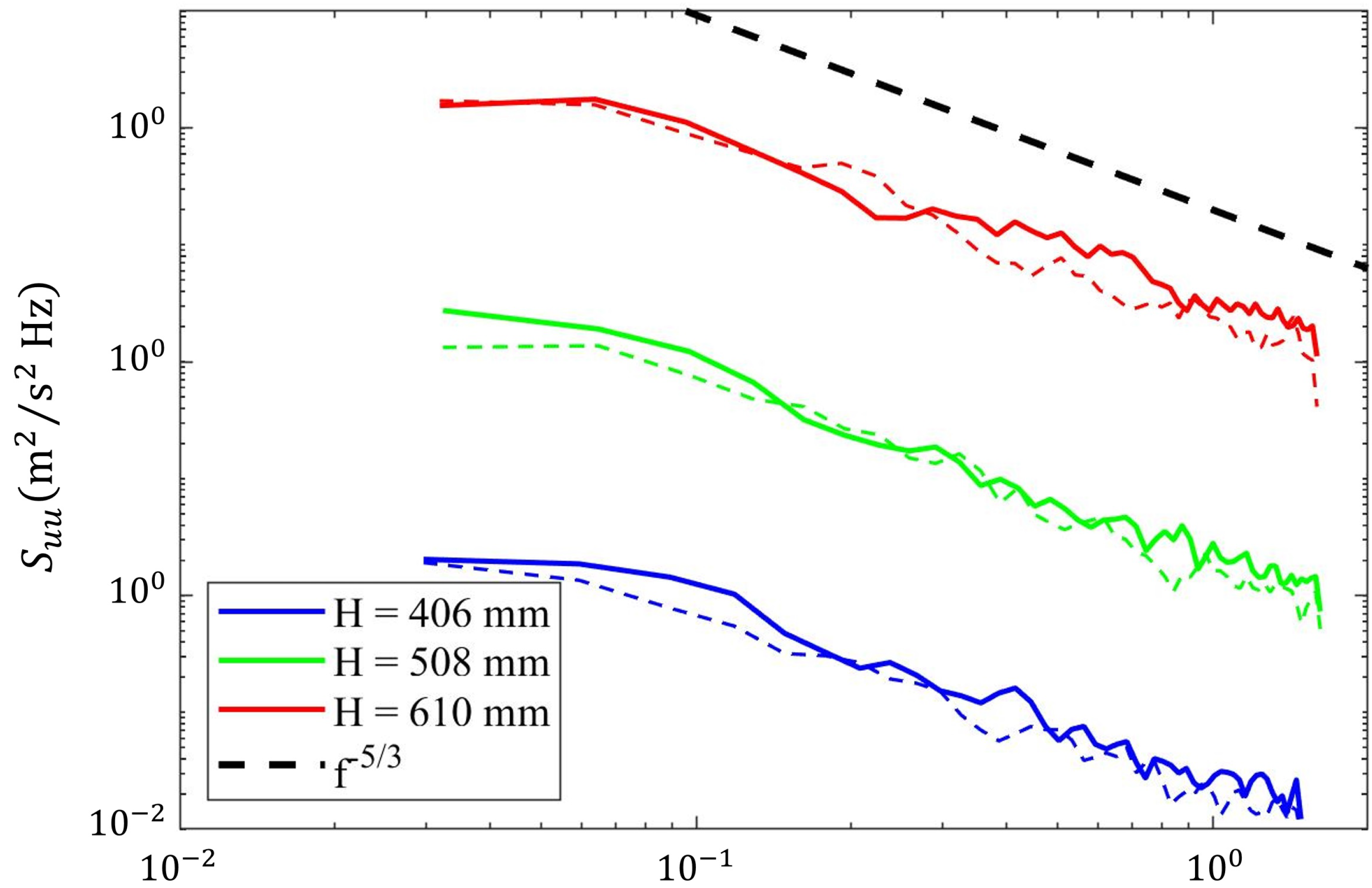
3.1. Laboratory Results
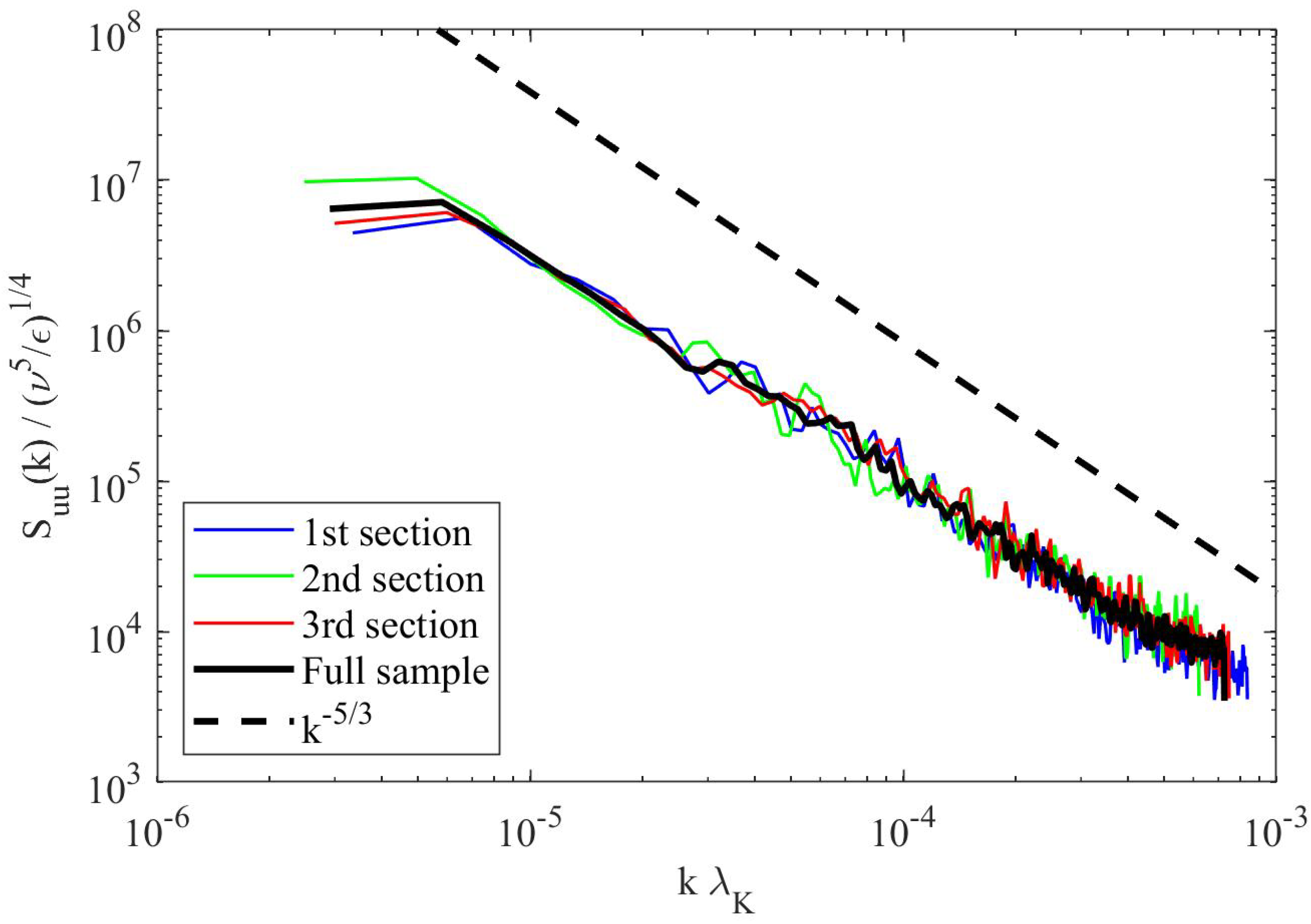
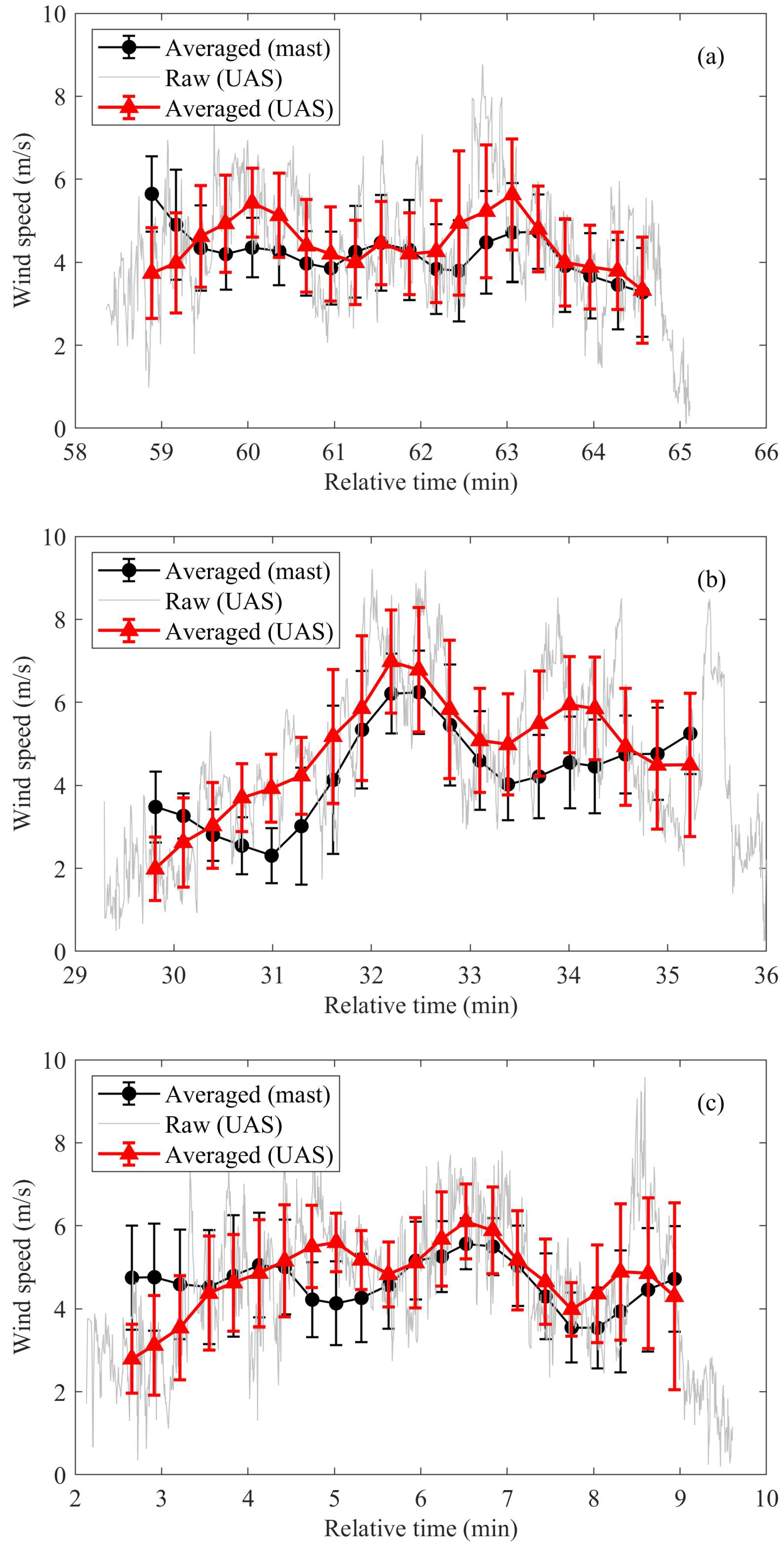
As previously discussed, the laboratory tests used PIV measurements in a water tunnel to examine the velocity field above (or below for the current test configuration) various rotor configurations. For each test configuration (dual parallel, dual perpendicular, quad-X, quad-plus) the velocity field was measured at three planes, two tunnel speeds (0 and 0.5 m/s), and three inclination angles (0, 15, and 30 deg). A complete presentation of each of these individual tests is provided in Brenner [22]. However, here a representative condition is examined and a summary of observations from individual test conditions is provided. Figure 4 shows the vector field from the quad-X configuration with 0 deg tilt and the laser aligned with the hub (see Figure 2). Overlaid with the velocity vector field is a sketch showing the side view of the rotor, which the rotors are downward facing following the laboratory testing orientation. Here a mean flow of 0.5 m/s was observed away from the rotor, while a significant vertical velocity component was induced by the rotors. The peak vertical component was 120% of the inlet streamwise (i.e., horizontal) velocity. It should be noted that the PIV measurements at 0.5 m/s matched the established tunnel performance within measurement uncertainty for nearly every case (there were two conditions where deviations were noted and these conditions were not used in subsequent analysis).
Since the rotor induced velocity would primarily be the vertical component, streamwise (X) profiles of the vertical velocity were extracted for further analysis. The corresponding profile for the vector field example is also provided in Figure 4 along with the profiles for the mid-plane and hub positions. The profiles are an average of the 3 rows of vectors centered on the dashed line going through the vector field in Figure 4. Consistent with the vector field, there is a very large peak in vertical velocity into the rotors near the rotor center for the hub plane. The profile extracted from the tip location also has a significant spike in vertical velocity into the rotor, though significantly reduced relative to the hub location. Conversely, the mid-plane shows much weaker velocity in the center with only a weak outward (i.e., away from the rotor) velocity component.
In general, tilting of the rotor for a given configuration simply shifted the velocity variations (peaks and valleys in the profiles) without having significant impact on the trends. The highest vertical velocities were observed over the rotors with a significant decrease in between rotors. The dual perpendicular configuration was initially quite informative. It showed that the vertical velocity was the lowest in the mid-plane while producing large peaks over the rotors. This gave an indication that between rotors is a region of relatively low velocity induction by the rotors. The quad-plus configuration results were consistent with this assessment, though it was more difficult to identify due to the center region also being aligned in the streamwise direction with the leading and trailing rotors. The quad-X results are more apparent with the mid-plane showing only weak vertical rotor induced velocity. This is shown in Figure 5 where the peak magnitude of vertical velocity is plotted versus rotor angle for each plane with the water tunnel speed set at 0 and 0.5 m/s. The peak vertical velocity was located within one rotor diameter above the model. The error bars are set at nominally twice the standard deviation of the uncertainty. Figure 5 also shows that the mid-plane peak velocity is lower than all other conditions besides one ( 0.5 m/s tip at 15 deg). However, the difference between these two conditions was within the measurement uncertainty. The overall maximum velocities were lower with the quad-X configuration than the dual perpendicular despite the presence of two additional rotors. This gives additional support to the value of locating measurements between rotors as the behavior suggests that the pairing mitigates the induced velocity. It should also be noted that for some configurations, the hub and tip measurements also produced negligible vertical velocity variation (sometimes even weaker than that between rotors). However, the low induced vertical velocities for the hub and tip locations would have steep spatial velocity gradients that make them extremely sensitive to the operation condition. Meaning this result was not consistent when operating conditions were varied (i.e., a change in rotor angle). Conversely, the spatial gradients in vertical velocity for regions between rotors were weaker and thus resulting in these regions being relative insensitive to the operating conditions (i.e., low induced velocity regardless of configuration, speed, or tilt).
Prior to field testing, a single rotor experiment was also performed in an ambient chamber. Here an anemometer was traversed across the rotor at various distances above it (rotor now oriented upward facing like traditional flight). Profiles were acquired at 200, 280, 330, 390, 430, and 480 mm above the rotor. The resulting velocity profiles at each height are shown in Figure 6. Each data point is an average from a 30 s period. Consistent with the PIV study, the highest velocities occur directly above the rotor hub. These results show a significant drop in the induced velocity at approximately 280 m above the rotor. The peak velocity continues to decrease with increasing height, but at a slower rate until the peak has decayed to 0.2 m/s at 480 mm above the rotor. Based on this asymptotic behavior, it was decided that fielding testing should have at least ∼400 mm standoff above the rotor plane. Field testing would then focus on increasing the height beyond 400 mm to assess the trade-off between decreasing rotor influence and decreasing platform stability.

3.2. Field Results

3.2.1. Mast Data

Field testing was performed near Stillwater, Oklahoma on three separate days in 2021 (10 May, 12 May, and 13 May). The current study focuses primarily on the data acquired on 10 May 2021, which was when data were acquired with the ultrasonic anemometer mounted in the center region above the four rotors (i.e., the preferred position as determined from the laboratory testing). The interested reader is referred to Brenner [22] to review field data acquired from the other days with the anemometer positioned at less ideal locations. The full 67 min time trace of the wind speed data acquired on the mast is shown in Figure 7. The average sample rate from the ultrasonic anemometer during the hour long period was 3.8 Hz. It should be noted that there were minor variations in the sample rate through the test, however, every data point was individually time stamped. The time is measured relative to the start of data acquisition on the mast, which was at 20:16:41 UTC (15:16:41 CDT) on 10 May 2021. Figure 7 includes the raw data as well as the average from a 2 min non-overlapping window. The averaging period was identified using the trial-and-error method for nonstationary single records [27], which identifies the period sufficiently large to reduce random error without creating significant bias error. The error bars are set at ± 1 standard deviation, with the standard deviation of each window varying between 0.71 and 1.81 m/s. The average wind speed for the entire period was 4.19 m/s, but there was significant fluctuations in wind speed during the measurement period with the minimum and maximum speeds being 0.48 and 10.4 m/s. However, the average from within any 2 min window only varied between 2.78 and 5.42 m/s with an average standard deviation 1.12 m/s.
The fluctuating (turbulence) statistics were then analyzed by dividing the mast time trace into three equal intervals of 1340 s (22.3 min). Each interval was segmented into 500 s windows with 75% overlap. The windowed segment was detrended with a linear fit to create a zero-mean time trace while mitigating the impact of temporal variation in the mean. A Hann window function was applied to the windowed segment to minimize the impact of truncating the time segment on the spectral content. Then the single-sided power spectral density was computed using the fast Fourier transform of the windowed time series. All of the power spectral densities for the window segments within a given 22.3 min interval were then averaged together to produce the mean power spectral density for the given interval. The temporal spectrum was converted to a spatial spectrum by invoking Taylor’s frozen turbulence hypothesis ( k U ω ; S u u ( k ) U S u u ( ω ) ). Here k ( = 2 π / λ ) is the wavenumber, λ is the wavelength, U is the mean wind speed, ω ( = 2 π f ) is the angular frequency, f is the temporal frequency, and S u u is the power spectral density of the wind speed ( u ) .
The conversion to a spatial spectrum allows the use of the K41 theory [28,29,30] to scale the spectra. K41 [28,29,30] uses physical reasoning to conclude that if the turbulence is locally homogeneous, isotropic, and stationary then the turbulent kinetic energy (TKE) at a given scale should only depend on the kinematic viscosity ( ν ) and the dissipation rate per unit mass ( ϵ ). Dimensional reasoning then leads to characteristic time, velocity, and length ( λ k = ( ν 3 / ϵ ) 1 / 4 ) scales. Consequently, the scaling of the spatial turbulence spectrum leads to S u u ( k ) / ( ν 5 / ϵ ) 1 / 4 being a function of k λ k . This scaling has been applied to the current mast spatial spectra and presented in Figure 8. The dissipation rate is difficult to determine, but it must be proportional to the rate that energy is supplied to the turbulence, ϵ U 3 / H m . Here U is the mean wind speed and H m is the height of the mast (i.e., it is being assumed that the largest eddies are proportional to the distance from the ground). In the current work, ϵ was set to be equal to 0.1 U 3 / H m , where the proportionality constant (0.1) was selected based on previous experimental observations [31]. The air temperature at 9-m measured from the Stillwater Oklahoma Mesonet station [32,33] was 15.1   ±   0.6 C, which sets the nominal kinematic viscosity at 1.5 × 10 5 m 2 / s. Each of the three scaled intervals collapse on nominally the same curve, which for comparison the spectra was also computed for the entire 67 min.
For eddies that are large compared to viscous scales and small compared to production scales (i.e., inertial scales) the energy dissipation rate should be independent of viscosity. This leads to the famous 5 / 3 law that states S u u ( k ) ϵ 2 / 3 k 5 / 3 . The dashed line in Figure 8 has a k 5 / 3 slope, which the current results do not follow this curve having a slope of k 4 / 3 . While the measurements are at very large Reynolds numbers, the sample rate ( 3.8 Hz) is relatively low. Consequently, it is informative to investigate where it is expected that these measurements should be in the inertial subrange. Saddoughi and Veeravalli [34] examine the scaling of high Reynolds number turbulent flows and show that even at very high Reynolds numbers the spectra deviate from the k 5 / 3 curve when k λ k < 10 4 . Thus, the current results having a slope below k 5 / 3 indicates that they are slightly outside of the inertial range, which is consistent with laboratory turbulence results in the literature.
While the current study focuses on the measurements acquired on 10 May 2021, for completeness the statistics from all three test days are also included here. The mean, variance, skewness, and kurtosis from the mast for each test day is provided in Table 1. The mean wind speeds varied between days, which is expected since local atmospheric conditions vary daily. While there was significant variation in the mean and fluctuations (variance) between days, the ratio of the fluctuating to mean velocity ( σ / U ) had less variation. Similarly, the higher order statistics (skewness and kurtosis) have negligible day to day variation. Each day appears to have slightly positive skewness, which indicates that the distribution is weakly skewed towards lower values. The kurtosis ( κ 2.8 ) is close to a normal distribution ( κ = 3 ).
The correlation function is also commonly used to define two turbulence scales, the integral and Taylor time (or spatial) scales. There is insufficient resolution to quantify the Taylor scale, which is a measure of how long the flow remains correlated with itself. The integral time scale is a measure of how long it takes for the flow to become uncorrelated with itself. The correlation of the fluctuating velocity signal is defined as R i j ( τ ) = u i ( t ) u j ( t + τ ) ¯ , where u i ( t ) and u j ( t ) are the velocity of the i th and j th, respectively, velocity components, t is the time, τ is the shifted time, and the overbar denotes the ensemble average. The autocorrelation ( R i i ) is used to define the integral time scale ( Λ t ),
Λ t = 1 R i i ( 0 ) 0 R i i ( τ ) d τ ,
where R i i ( 0 ) is equal to the sample variance. The computed integral time scales are also included in Table 1. While the integral time scale is difficult to quantify given the unsteadiness within the surface layer, the general trend shows increasing integral scales with decreasing mean wind speeds. This is consistent with expectations given higher Reynolds numbers (i.e., higher speeds) would have finer scales.

3.2.2. UAS Data

Data was acquired on the UAS from the front, back, and middle positions at all of the test heights (406, 508, 610 mm) above the rotors, but as stated previously the focus of the current study is on results from the middle position. These data were acquired on 10 May 2021, but the interested reader is referred to Brenner [22] for results from the additional conditions. The periods of time when the UAS was acquiring data are marked with the shaded regions in Figure 7. The 610, 508, and 406 mm heights began recording at 2.1, 29.3, and 58.4 min relative to 10 May 2021 20:16:41 UTC. The individual raw time traces of the wind speeds measured on the UAS are shown in Figure 9. Figure 9 also includes the average wind speed from the UAS and the mast for a 1 min window with 70% overlap between windows. The shorter window and increased overlap relative to that shown in Figure 7 is due to the shorter sampling period of the UAS. The error bars are set at ± 1 standard deviation for the given window. The overall average (standard deviation) from the UAS for the 406, 508, and 610 mm heights above the rotor are 4.22 m/s (1.23 m/s), 4.33 m/s (1.51 m/s), and 4.56 m/s (1.22 m/s), respectively. The comparison between the mast and UAS as well as the trends in the data are provided subsequently in Section 4.
The power spectral density was computed from the UAS measurements for each anemometer height (406, 508, and 610 mm). The spectrum for each height are plotted in Figure 10 with the origin shifted for each spectra to make comparison between each height and the corresponding mast data more apparent. Each spectral curve (UAS at various heights and the corresponding mast data) was produced by first segmenting the given interval into 100-s windows with 75% overlap. The windowed segment was detrended with a linear fit, and then a Hann function was applied. The power spectral density for each window was computed and then the average of all windowed segments is plotted in Figure 10. Unlike the presentation of the mast data, the spectra are not scaled following K41 theory, this was done so that the direct comparison between mast and UAS data is more readily interpreted. However, a reference curve with a slope of 5 / 3 power is still included as a reference. Similar to the mast data, the slope of the UAS measurements are slightly lower than the 5 / 3 power curve, which is expected given the scaled frequency/wavenumber (see Figure 8). Fitting of the power spectral density points when k λ k 10 4 for each measurement height shows that the spectral slope was 1.42 ± 0.08 , which shows that the fluctuating spectral content was relatively consistent between segments even though there was nearly 20 min between UAS samples.

4. Discussion

A summary of the wind speed statistics acquired from the mast and the UAS with the anemometer positioned in the middle of the rotors is provided in Table 2. Table 2 also includes a percent difference of each statistic, which is defined as the difference between UAS-based statistic and the mast-based statistic divided by the mast-based statistic (i.e., the trusted measurement). The variation in the mean wind speeds can be compared by examining the averaged data plotted in Figure 9. This shows that for each measurement period there are segments where the trends are in good agreement between the two sensors, such as at a height of 508 mm (Figure 9b) from 31 t r 33 min and at a height of 610 mm (Figure 9c) from 6 t r 8 min. However, it is apparent that over these same segments there is a bias error between the UAS and mast based sensors. To better quantify the deviation in measurements, the absolute difference between the mast based and UAS based 1 min averages, | u m ¯ u u a s ¯ | , was computed, where the -brackets indicate average over the entire measurement period and the overbar indicates average over the 1 min window. These values are also listed in Table 2. Both the percent difference and the absolute difference show that the largest deviation occurred at a height of 508 mm. A likely source of error in these measurements is due to wind shear because the height was manually matched by the operator on the ground, which there was estimated to be about 0.3 m difference. Use of a Mesonet tower [32,33] 1.6 km from the test site showed that the average wind shear during testing was 0.111 s 1 ± 0.047 s 1 , which would create average deviations in the wind speed of up to 0.05 m/s over a 0.3 m separation. This percent difference for 508 mm condition corresponds to a speed difference of 0.24 m/s, which is too large to be explained simply by the mean wind shear. However, the Mesonet wind shear measurements are 5 min averages and the above estimate was for the entire duration of testing, but point by point measurements show that the wind shear spiked at the same time of the 508 mm measurement. This conjecture is further supported by the observation that the deviations in the mean do not decrease with increasing separation distance. There are other segments within each measurement period in Figure 9 when the trends do not appear to be in agreement, such as the first and last minute at a height of 508 mm (Figure 9b) where the slopes are opposite between the mast and the UAS sensors. The source for such discrepancies cannot be assessed from this data set due to the relatively short sample period with the UAS and the fact that the two measurements could not be at the same physical location (i.e., there is a reasonable chance that both were correct and this is a measure of the spatial variability over the 9.1 m separation).
The wind speed fluctuations (standard deviation in Table 2) were consistently larger with the UAS-based measurements relative to the mast-based measurements. This is expected since some of the UAS motions will cause an increase in measurement variability combined with the side-by-side comparison that showed the UAS anemometer was ∼10% larger. Of note, there is a trend of increasing percent difference in standard deviation scaled with the mean wind speed, σ / U , between the mast and the UAS with increasing sensor height. This could be due to the increasing separation distance having an impact on the UAS stability, but over the range of test conditions this impact was weak. The power spectral density is a means of separating the frequency content of the variance ( σ 2 ), which when applying Taylor’s frozen turbulence hypothesis allows it to be interpreted as a spatial distribution of eddies of various sizes. Figure 10 allows the UAS-based (solid curves) and mast-based (dashed curves) spectral content to be compared. This shows that the H = 610 mm condition had the largest variation between the mast and the UAS sensors, but overall all three measurements produces very similar results. Higher order statistics are also compared in Table 2. The percent differences for skewness are large, but this is more an indication that both measurements show negligible skewness (i.e., the distribution is nearly symmetric with a skewness close to zero) in the data. The kurtosis is close between the mast and the UAS data with the exception of the measurement 406 mm above the rotors. The UAS based measurement with the 406 mm offset is the outlier relative to all other kurtosis measurements as it was 3.21 compared to 2.41 ± 0.26 for all other measurements from the UAS and the mast.

5. Conclusions

This study further analyzed data originally presented in Brenner [22], which includes laboratory and field testing. The majority of the laboratory testing used PIV to examine the horizontal distribution of vertical velocity above various rotor configurations with and without a mean flow applied. These results showed that the rotor tilting shifted the results but had minimal impact on the observed trends. The rotors generally had the weakest influence on the measured flow-field in the region in between pairs of rotors. There were other locations (hub and tip) that observed low disturbances, but these locations had steep spatial gradients, which would make the resulting measurements very sensitive to variations in operational conditions. Consequently, it was concluded that positioning sensors on quad-copters near the center of the UAS above the rotors would be ideal. There was also a simple single rotor test to examine the vertical variation in the disturbed velocity field since the PIV testing was constrained in the vertical direction. The single rotor test indicates that within 280 mm (3.7 rotor diameters) there are large induced velocities by the rotor. Measurements were extended to 480 mm above the rotor, which the profiles indicate a relatively weak disturbance beyond ∼400 mm. A sketch of the preferred location for wind speed measurements from a quad-copter UAS based on the laboratory testing is provided in Figure 11.
Field testing was performed with a quad-copter UAS hovering 9.1 m above the ground and 9.1 m separation between it and a mast with an ultrasonic anemometer 9.1 m above the ground. The UAS had a lightweight ultrasonic anemometer mounted at various heights (406, 508, 610 mm) above the rotors. Brenner [22] varied the mounting position, but the current study only focused on the data acquired with the sensor mounted in between both pairs of rotors. Analysis of the mean, variance, and higher order statistics show that the UAS-based wind speed measurements produced similar results to that acquired on a fixed mast. The difference in the mean values are conjectured to be the product of mean shear coupled with poor precision in positioning the UAS height during the test. This was true regardless of the separation height above the UAS, thus indicating that 406 mm (5.3 rotor diameters) was sufficient separation to have minimal impact from the rotors on the mean wind speed measurements when positioned between rotors. The results compare well with similar studies, such as Ingenhorst et al. [35], which found very good agreement with reference data, including both mean wind speeds and wind directions during position-controlled hovering. Though rotor influences were not evaluated in Ingenhorst et al. [35], they determined that turbulence intensity estimation was ‘reasonably good’. These results are promising preliminary results but requires additional field measurements. It is recommended that future tests directly quantify the local shear, GPS be used to precisely locate the UAS relative to the mast or tower, acquire multiple measurement periods for each configuration, and examine sensitivity to platform design (i.e., rotor sizing, spacing, etc.).

Author Contributions

Conceptualization, J.B. and J.D.J.; Formal analysis, T.C.W., Z.M. and B.R.E.; Funding acquisition, J.D.J. and B.R.E.; Investigation, T.C.W., J.B., J.D.J. and B.R.E.; Methodology, J.B. and J.D.J.; Project administration, J.D.J.; Resources, J.D.J.; Supervision, J.D.J. and B.R.E.; Visualization, J.B. and B.R.E.; Writing—original draft, J.B. and J.D.J.; Writing—review and editing, T.C.W., Z.M. and B.R.E. All authors have read and agreed to the published version of the manuscript.

Funding

This research was funded in part by the National Aeronautics and Space Administration (NASA) University Leadership Initiative (ULI) program under grant number 80NSSC20M0162, Weather Intelligent Navigation Data and Modeling for Aviation Planning (WINDMAP) and the National Science Foundation (USA) under grant number 1925147, NRI: INT: Safe Wind-Aware Navigation for Collaborative Autonomous Aircraft in Low Altitude Airspace.

Institutional Review Board Statement

Not applicable.

Informed Consent Statement

Not applicable.

Data Availability Statement

The data presented in this study are available on request from the corresponding author.

Acknowledgments

The authors would like to acknowledge Andrew Quinton and Kyle Hickman for their assistance with PIV experiments and flight testing of sensors and aircraft, respectively.

Conflicts of Interest

The authors declare no conflict of interest.

References

  1. Durre, I.; Vose, R.S.; Wuertz, D.B. Overview of the Integrated Global Radiosonde Archive. J. Clim. 2006, 19, 53–68. [Google Scholar] [CrossRef] [Green Version]
  2. Nambiar, M.K.; Byerlay, R.A.; Nazem, A.; Nahian, M.R.; Moradi, M.; Aliabadi, A.A. A Tethered Air Blimp (TAB) for Observing the Microclimate over a Complex Terrain. Geosci. Instrum. Methods Data Syst. 2020, 9, 193–211. [Google Scholar] [CrossRef]
  3. Byerlay, R.A.E.; Nambiar, M.K.; Nazem, A.; Nahian, M.R.; Biglarbegian, M.; Aliabadi, A.A. Measurement of Land Surface Temperature from Oblique Angle Airborne Thermal Camera Observations. Int. J. Remote Sens. 2020, 41, 3119–3146. [Google Scholar] [CrossRef]
  4. Nahian, M.R.; Nazem, A.; Nambiar, M.K.; Byerlay, R.; Mahmud, S.; Seguin, A.M.; Robe, F.R.; Ravenhill, J.; Aliabadi, A.A. Complex Meteorology over a Complex Mining Facility: Assessment of Topography, Land Use, and Grid Spacing Modifications in WRF. J. Appl. Meteorol. Climatol. 2020, 59, 769–789. [Google Scholar] [CrossRef]
  5. Hemingway, B.; Frazier, A.E.; Elbing, B.R.; Jacob, J.D. Vertical sampling scales for atmospheric boundary layer measurements from small unmanned aircraft systems (sUAS). Atmosphere 2017, 8, 176. [Google Scholar] [CrossRef] [Green Version]
  6. Smith, S.W.; Chilson, P.B.; Houston, A.L.; Jacob, J.D. Catalyzing collaboration for multi-disciplinary UAS development with a flight campaign focused on meteorology and atmospheric physics. In Proceedings of the AIAA Information Systems, Grapevine, TX, USA, 9–13 January 2017; AIAA-2017-1156. [Google Scholar]
  7. Jacob, J.D.; Chilson, P.B.; Houston, A.L.; Smith, S.W. Considerations for atmospheric measurements with small unmanned aircraft systems. Atmosphere 2018, 9, 252. [Google Scholar] [CrossRef] [Green Version]
  8. Koch, S.E.; Fengler, M.; Chilson, P.B.; Elmore, K.L.; Argrow, B.; Andra, D.L., Jr.; Lindley, T. On the Use of unmanned aircraft for sampling mesoscale phenomena in the preconvective boundary layer. J. Atmos. Ocean. Technol. 2018, 35, 2265–2288. [Google Scholar] [CrossRef]
  9. Barbieri, L.; Kral, S.T.; Bailey, S.C.C.; Frazier, A.E.; Jacob, J.D.; Reuder, J.; Brus, D.; Chilson, P.B.; Crick, C.; Detweiler, C.; et al. Intercomparison of small unmanned aircraft system (sUAS) measurements for atmospheric science during the LAPSE-RATE campaign. Sensors 2019, 19, 2179. [Google Scholar] [CrossRef] [Green Version]
  10. González-Rocha, J.; Woolsey, C.A.; Sultan, C.; De Wekker, S.F.J. Sensing wind from quadrotor motion. J. Guid. Control Dyn. 2019, 42, 836–852. [Google Scholar] [CrossRef]
  11. Greene, B.R.; Segales, A.R.; Bell, T.M.; Pillar-Little, E.A.; Chilson, P.B. Environmental and sensor integration influences on temperature measurements by rotary-wing unmanned aircraft systems. Sensors 2019, 19, 1470. [Google Scholar] [CrossRef] [PubMed] [Green Version]
  12. Natalie, V.A.; Jacob, J.D. Experimental observations of the boundary layer in varying topography with unmanned aircraft. In Proceedings of the AIAA Aviation Forum, Dallas, TX, USA, 17–21 June 2019; AIAA-2019-3404. [Google Scholar]
  13. Frew, E.W.; Argrow, B.; Borenstein, S.; Swenson, S.; Hirst, C.A.; Havenga, H.; Houston, A. Field observation of tornadic supercells by multiple autonomous fixed-wing unmanned aircraft. J. Field Robot. 2020, 37, 1077–1093. [Google Scholar] [CrossRef]
  14. Hemingway, B.; Frazier, A.E.; Elbing, B.R.; Jacob, J.D. High-resolution estimation and spatial interpolation of temperature structure in the atmospheric boundary layer using a small unmanned aircraft system. Bound.-Layer Meteorol. 2020, 175, 397–416. [Google Scholar] [CrossRef]
  15. Elston, J.; Argrow, B.; Stachura, M.; Weibel, D.; Lawrence, D.; Pop, D. Overview of Small Fixed-Wing Unmanned Aircraft for Meteorological Sampling. J. Atmos. Ocean. Technol. 2015, 32, 97–115. [Google Scholar] [CrossRef]
  16. Whyte, S.; Jacob, J. Experimental Measurement of Flow Field Around a Rotary Wing Unmanned Aircraft. Bull. Am. Phys. Soc. 2018, 63, E14-2. [Google Scholar]
  17. Yoon, S.; Diaz, P.V. High-Fidelity Computational Aerodynamics of Multi-Rotor Unmanned Aerial Vehicles. In Proceedings of the AIAA SciTech, Kissimmee, FL, USA, 8–12 January 2018; AIAA-2018-1266. [Google Scholar]
  18. Anke Rau, G. Two New Technologies to Measure the Turbulent Wind Vector Aboard Small Research UAV. Master’s Thesis, Eberhard Karls University Tübingen, Tübingen, Germany, 2016. [Google Scholar]
  19. Bruschi, P.; Piotto, M.; Dell’Agnello, F.; Ware, J.; Roy, N. Wind Speed and Direction Detection by Means of Solid-State Anemometers Embedded on Small Quadcopters. Procedia Eng. 2016, 168, 802–805. [Google Scholar] [CrossRef]
  20. Vasiljevic, N.; Harris, M.; Tegtmeier Pedersen, A.; Rolighed Thorsen, G.; Pitter, M.; Harris, J.; Bajpai, K.; Courtney, M. Wind sensing with drone-mounted wind lidars: Proof of concept. Atmos. Meas. Tech. 2020, 13, 521–536. [Google Scholar] [CrossRef] [Green Version]
  21. Leuenberger, D.; Haefele, A.; Omanovic, N.; Fengler, M.; Martucci, G.; Calpini, B.; Fuhrer, O.; Rossa, A. Improving high-impact numerical weather prediction with lidar and drone observations. Bull. Am. Meteorol. Soc. 2020, 101, E1036–E1051. [Google Scholar] [CrossRef] [Green Version]
  22. Brenner, J. Inflow Analysis for Multi-Rotors and the Impact on Sensor Placement. Master’s Thesis, Oklahoma State University, Stillwater, OK, USA, 2021. [Google Scholar]
  23. Lucido, N.A.; KC, R.J.; Wilson, T.C.; Jacob, J.D.; Alexander, A.S.; Elbing, B.R.; Ireland, P.; Black, J.A., III. Laminar boundary layer scaling over a conformal vortex generator. In Proceedings of the AIAA SciTech Forum, San Diego, CA, USA, 7–11 January 2019; AIAA2019-1135, pp. 1–11. [Google Scholar]
  24. Niemiec, R.; Gandhi, F. A comparison between quadrotor flight configurations. In Proceedings of the 42nd European Rotorcraft Forum, Lille, France, 5–7 September 2016. [Google Scholar]
  25. Reich, D.; Sinding, K.; Schmitz, S. Visualization of a helicopter rotor hub wake. Exp. Fluids 2018, 59, 116. [Google Scholar] [CrossRef]
  26. Petrin, C.E.; Jayaraman, B.; Elbing, B.R. Characterization of a canonical helicopter hub wake. Exp. Fluids 2019, 60, 9. [Google Scholar] [CrossRef] [Green Version]
  27. Bendat, J.S.; Piersol, A.G. Random Data: Analysis and Measurement Procedures, 3rd ed.; John Wiley & Sons, Inc.: Hoboken, NJ, USA, 2000; pp. 457–477. [Google Scholar]
  28. Kolmogorov, A.N. The local structure of turbulence in incompressible viscous fluid for very large Reynolds numbers. Dokl. Akad. Nauk. SSSR 1941, 30, 9–13. [Google Scholar]
  29. Kolmogorov, A.N. On degeneration (decay) of isotropic turbulence in an incompressible viscous liquid. Dokl. Akad. Nauk. SSSR 1941, 31, 538–540. [Google Scholar]
  30. Kolmogorov, A.N. Dissipation of energy in locally isotropic turbulence. Dokl. Akad. Nauk. SSSR 1941, 32, 16–18. [Google Scholar]
  31. Friehe, C.A.; Van Atta, C.W.; Gibson, C.H. Jet Turbulence: Dissipation rate measurements and correlations. AGARD Turbul. Shear. Flows 1971, CP-93, 18. [Google Scholar]
  32. Brock, F.V.; Crawford, K.C.; Elliott, R.L.; Cuperus, G.W.; Stadler, S.J.; Johnson, H.L.; Eilts, M.D. The Oklahoma Mesonet: A technical overview. J. Atmos. Ocean. Technol. 1995, 12, 5–19. [Google Scholar] [CrossRef]
  33. McPherson, R.A.; Fiebrich, C.; Crawford, K.C.; Elliott, R.L.; Kilby, J.R.; Grimsley, D.L.; Martinez, J.E.; Basara, J.B.; Illston, G.G.; Morris, D.A.; et al. Statewide monitoring of the mesoscale environment: A technical update on the Oklahoma Mesonet. J. Atmos. Ocean. Technol. 2007, 24, 301–321. [Google Scholar] [CrossRef] [Green Version]
  34. Saddoughi, S.; Veeravalli, S. Local isotropy in turbulent boundary layers at high Reynolds number. J. Fluid Mech. 1994, 268, 333–372. [Google Scholar] [CrossRef]
  35. Ingenhorst, C.; Jacobs, G.; Stößel, L.; Schelenz, R.; Juretzki, B. Method for airborne measurement of the spatial wind speed distribution above complex terrain. Wind Energy Sci. 2021, 6, 427–440. [Google Scholar] [CrossRef]
Figure 1. Example of common multi-rotor system operated by the Unmanned Systems Research Institute (USRI, Stillwater, OK, USA) with an instrumentation suite that includes sensors for pressure, humidity, temperature, wind speed, and gas concentration.
Atmosphere 13 00443 g001
Figure 2. (top) Sketch of the test section layout for the water tunnel testing. Below the sketch from top to bottom is the test orientations for the dual perpendicular, dual parallel, quad-X, and quad-plus configurations. In each configuration the left column is a bottom view, right are the three angles tested, and the flow is left to right. The three horizontal green lines mark in each configuration the laser planes termed the (T) tip, (H) hub, and (M) mid-plane.
Atmosphere 13 00443 g002
Figure 3. (left) Layout for fielding testing with the SKB-1000 relative to the Blue Sky Mast. (right) Model of the SKB-1000 with the front, middle, and back post positions. The post length was also varied during testing.
Atmosphere 13 00443 g003
Figure 4. (left) PIV vector field from 0.5 m/s condition using the quad-X configuration with the laser plane aligned with the hub and the model oriented with 0 deg tilt. The color map corresponds the vertical velocity (V) and the black arrows are the measured vectors. (right) The vertical velocity (V) profile extracted from the condition on the left marked with a thin dashed white line through the vector field as well as the same condition at the mid and tip planes.
Atmosphere 13 00443 g004
Figure 5. Peak magnitude vertical velocity into the rotor for the Quad-X configuration with the flow at (dashed) 0 m/s or (solid) 0.5 m/s and varying rotor angles at the hub, mid, and tip planes.
Atmosphere 13 00443 g005
Figure 6. Profiles (vertical and horizontal) of the average vertical velocity induced by a single stationary rotor. Each data point was the average from a 30 s period.
Atmosphere 13 00443 g006
Figure 7. Time trace of wind speed measured on the fixed mast on 10 May 2021. The averaged mast data (thick black curve) is the average from a 2 min non-overlapping window. The error bars are equal to the standard deviation from the given window. Shaded green windows indicate the period of time when UAS data were acquired.
Atmosphere 13 00443 g007
Figure 8. The turbulence spectral density scaled following the K41 theory [28,29,30]. The dashed curve has a slope of k 5 / 3 for reference.
Atmosphere 13 00443 g008
Figure 9. Time trace of the raw and average wind speed measurements from the UAS in the field near the mast with the anemometer located (a) 406 mm, (b) 508 mm, and (c) 610 mm above the rotors. The corresponding mast data with the same window (60 s) and overlap (70%) are included for reference. Error bars are ± 1 standard deviation for each 60-s window. All times are shown relative to the start of the mast data acquisition at 20:16:41 UTC on 10 May 2021.
Atmosphere 13 00443 g009
Figure 10. The power spectral density from the UAS with the anemometer positioned at 406, 508, or 610 mm above the rotors. Dashed curves are the power spectral density measured on the mast for the same time interval as the corresponding UAS measurements. The origin of each curve has been shifted by two orders of magnitude to make the comparison more apparent.
Atmosphere 13 00443 g010
Figure 11. Sketch of the (upper) top view and (lower) side view illustrating the different regions observed in the laboratory testing to determine the ideal positioning of the wind speed sensors to mitigate the impact of the rotors on the measurement. The lower figures conceptualize comparative regions for a typical system in hovering flight in a (left) quiescent atmosphere and with a (right) cross-flow. The “clean” region above the in wash is shown by the approximate distance above the rotor plane of approximately 1.2 times the rotor diameter, R D .
Atmosphere 13 00443 g011
Table 1. Comparison of wind speed statistics from data acquired during May of 2021 from the ultrasonic anemometer on the fixed mast.
DateMean (U)Variance ( σ 2 ) σ / U Skewness (s)Kurtosis ( κ ) Λ t
(m/s)(m 2 / s 2 )(–)(–)(–)(s)
May 104.191.880.330.262.8217
May 122.581.160.420.282.8268
May 131.800.780.490.262.7493
Table 2. Comparison of wind speed statistics measured from the UAS or the fixed mast. The “Diff” is the percent difference between the UAS and mast statistic and divided by the mast value. In addition, absolute error is provided for each measurement with the angle bracket and overbar being averages over the entire measurement period and the 1 min window, respectively.
HeightSourceU σ σ / U s κ
(mm) (m/s)(m/s)(–)(–)(–)
406UAS, u u a s 4.251.400.330.103.21
Mast, u m 4.221.230.290.072.45
Diff0.7%13.8%13.8%42.9%31.0%
| u u a s ¯ u m ¯ | 0.54
508UAS, u u a s 4.571.960.430.232.23
Mast, u m 4.331.510.350.162.43
Diff5.5%29.8%22.9%43.8%−8.2%
| u u a s ¯ u m ¯ | 0.86
610UAS, u u a s 4.481.620.36−0.112.58
Mast, u m 4.561.220.270.132.35
Diff−1.8%32.8%33.3%184.6%9.8%
| u u a s ¯ u m ¯ | 0.64
Publisher’s Note: MDPI stays neutral with regard to jurisdictional claims in published maps and institutional affiliations.

