Article

Evaluation of Technology for the Analysis and Forecasting of Precipitation Using Cyclostationary EOF and Regression Method

1
Chinese Research Academy of Environmental Sciences, No. 8 Dayangfang, Anwai Beiyuan, Chaoyang District, Beijing 100012, China
2
Department of Civil Engineering, Kyungpook National University, Daegu 702701, Korea
*
Authors to whom correspondence should be addressed.
Atmosphere 2022, 13(3), 500; https://doi.org/10.3390/atmos13030500
Submission received: 15 January 2022 / Revised: 15 March 2022 / Accepted: 19 March 2022 / Published: 21 March 2022

Abstract

:
Precipitation time series exhibit complex fluctuations and statistical changes. Existing research stops short of a simple and feasible model for precipitation forecasting. In this article, the authors investigate and forecast precipitation variations in South Korea from 1973 to 2021 using cyclostationary empirical orthogonal function (CSEOF) and regression methods. First, empirical orthogonal function (EOF) and CSEOF analyses are used to examine the periodic changes in the precipitation data. Then, the autoregressive integrated moving average (ARIMA) method is applied to the principal component (PC) time series derived from the EOF and CSEOF precipitation analyses. The fifteen leading EOF and CSEOF modes and their corresponding PC time series clearly reflect the spatial distribution and temporal evolution characteristics of the precipitation data. Based on the PC forecasts of the EOF and CSEOF models, the EOF–ARIMA composite model and CSEOF–ARIMA composite model are used to obtain quantitative precipitation forecasts. The comparison results show that both composite models have good performance and similar accuracy. However, the performance of the CSEOF–ARIMA model is better than that of the EOF–ARIMA model under various measurements. Therefore, the CSEOF–ARIMA composite forecast model can be considered an efficient and feasible technology representing an analytical approach for precipitation forecasting in South Korea.

1. Introduction

Global climate and environmental changes have become major worldwide issues in recent years. In particular, interactions between the atmosphere and slowly changing oceans will have profound and long-term effects on humans. Because agricultural production and hydrological management are heavily influenced by the climate, meteorologists are interested in the effects of climate and environmental changes, such as variations in periodic meteorological phenomena [1].
Precipitation is an important variable in climate change research and significant in hydrological processes [2,3]. It is the main component of the water cycle and has a great influence on surrounding environments and hydrological systems. Changes in the timing and amount of precipitation in a given area can lead to serious flood hazards or agricultural failures due to floods and droughts. Because human-induced climate change accelerates the hydrological cycle of the ecosystem, forecasting precipitation on the decadal scale is becoming increasingly important for long-term water resource management [4,5]. Advanced precipitation forecasting technologies and timely precipitation diagnoses can help improve the operation of water storage facilities and prevent potential flood disasters. The latest Intergovernmental Panel on Climate Change report indicated that there is growing concern in the scientific community regarding the significant increases observed in the amount and intensity of precipitation and regarding the corresponding variations [6].
Much research has been conducted regarding forecasting precipitation, with many studies highlighting that the trends observed in the annual and monthly precipitation of different regions depend on the region of interest and the time period examined [7,8,9]. Several studies have focused on seasonal predictions of precipitation at the regional level using different technologies, such as regional climate models [10], in conjunction with other climate variables [11,12]. Some studies have improved the approaches used to forecast climate index values, such as projections with teleconnection indices [13] and the development of other ensemble forecasting models [14,15]. In addition, many studies have closely investigated the various trends and spatiotemporal characteristics of precipitation in South Korea [16,17,18,19].
Precipitation is measured by various observation systems on the ground and in space. Therefore, understanding the nature of measurement data is the basis for understanding uncertainty and reliability [20]. Weather radar provides the spatial distribution of precipitation estimation, but due to various natural factors, it will also be limited in estimating accurate precipitation [21]. The rain gauge data is considered to be real ground data because of its high quality, resolution and availability [22]. From this point of view, the research of rain gauge data and precipitation data set has many advantages, so it has a wide application prospect.
In general, traditional statistical methods are typically used for long-range forecasting, with the incorporation of dynamical methods contributing improvements. Some successful approaches have involved performing climate forecasting using multiple regression and correlation analysis methods. The Dynamical Climate Models have been used in SST Forecasts from 1997 to 1998 with precisely enough verification [23]. Seasonal prediction of coastal ocean conditions in the Atlantic have been evaluated by a higher skill Linear Inverse Model (LIM) [24]. The evolution and dynamic predictability of Madden–Julian oscillation (MJO) have been exploited and estimated in achieving the likely forecast potential in their own research [25,26].
Many climatic variables, such as precipitation, surface temperature, and solar flux, are known to exhibit periodic (annual, monthly, daily, etc.) variations in their statistical features. Analyses of such datasets performed using stationary approaches often yield meaningless statistical characteristics, representing the weak error correction performance of these methods and their inaccuracy in obtaining long-term predictions. Therefore, it is both appropriate and advantageous to adopt a cyclostationary methodology for statistical analyses of climatic phenomena that display strong cyclical trends.
Precipitation has typical cyclical variations with statistical fluctuations and seasonal tendencies. Particularly when a precipitation dataset covers several weather stations or spans different seasons, stationary methods can be used to obtain only the most obvious statistical trends. In climate studies, empirical orthogonal function (EOF) analyses are often used to study possible spatial patterns of variability and how these patterns change with time. Some studies have used EOF models to analyze precipitation data. Cahalan analyzed monthly precipitation data over the US and Canada based on EOFs and their variances [27]. Singh compared major rainfall patterns using the main modes of OLR data [28]. Svensson showed that most of the variance observed in rainfall in four periods could be explained by an elongated spatial rainfall pattern [29]. As such, EOF analyses are sometimes classified as multivariate statistical techniques. However, EOF analyses are not based on physical principles. Thus, to adequately analyze a comprehensive dataset, we use a cyclostationary empirical orthogonal function (CSEOF) analysis technique; this approach is useful for extracting evolving spatial patterns.
The existing scholarship in this field, however, tends to use complex system model or more input data and stays short of generalizing a simple and easy-to-use method for precipitation forecasting. This study primarily focuses on the analysis of the most dominant component of the seasonal cycle of precipitation in South Korea. Empirical orthogonal function (EOF) and CSEOF analyses are conducted to extract individual modes in the observed precipitation data to obtain the temporal and spatial evolution of individual synoptic fields. We use EOF and CSEOF analyses as the primary techniques to analyze the temporal evolution of the variability in precipitation and demonstrate the physical mechanism associated with each mode of precipitation variability. The autoregressive integrated moving average (ARIMA) model is used to examine and forecast the evolution of the temporal modes of precipitation variability derived from the EOF and CSEOF. Precipitation forecasts are generated from the regressed temporal and spatial patterns. The present study provides a detailed explanation of the observed changes in precipitation variables and explores a feasible statistical methodology for forecasting precipitation in a monsoon climate.
The data used in this study are described in Section 2. The EOF and CSEOF analysis methods used to analyze precipitation variability and the ARIMA model are also explained in Section 2. The cyclical seasonal characteristics of precipitation variability are presented in Section 3. The forecasting performance and related mechanisms are discussed in Section 4. Conclusions are presented in Section 5.

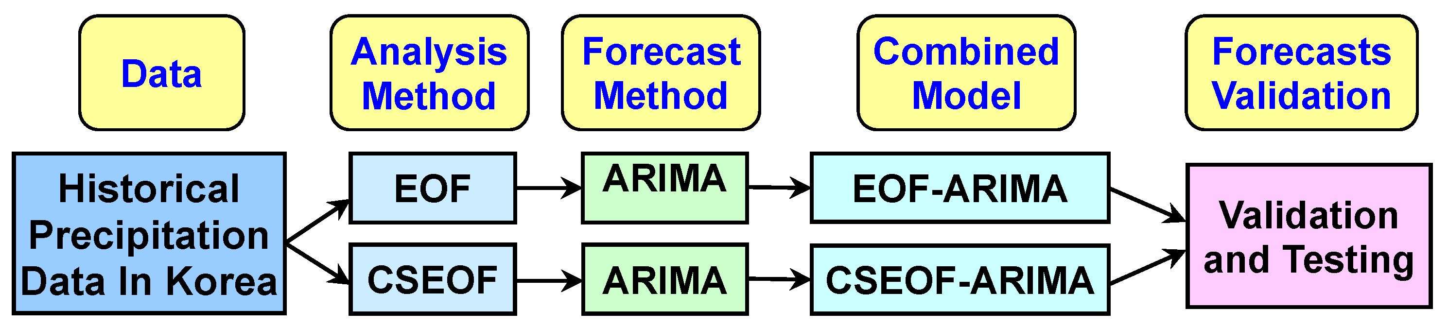
2. Data and Methodology

2.1. Data

The primary data used in the present study were precipitation measurements taken over South Korea by the Korea Meteorological Administration (KMA). A realtime quality control system was developed for meteorological data measured by integrated meteorological sensors based on a comparison of quality control procedures developed for meteorological data by the World Meteorological Organization and the KMA. The 56 weather stations from which the data analyzed in this study were collected are generally well distributed across the mainland, as shown in Figure 1, while data from Jejudo and Ulleungdo as well as some missing data were excluded from the analysis. The dataset represents the longest and most consistent precipitation observations available in South Korea, spanning 49 years (1973–2021). In this study, the data from the first 44 years (1973–2016) of the time series are used to generate the forecasting model, while the last five years (2017–2021) of precipitation records are used to validate the model.

2.2. Methodology

The statistical techniques used in this study are EOFs and CSEOFs for decomposing the data and ARIMA models for forecasting.

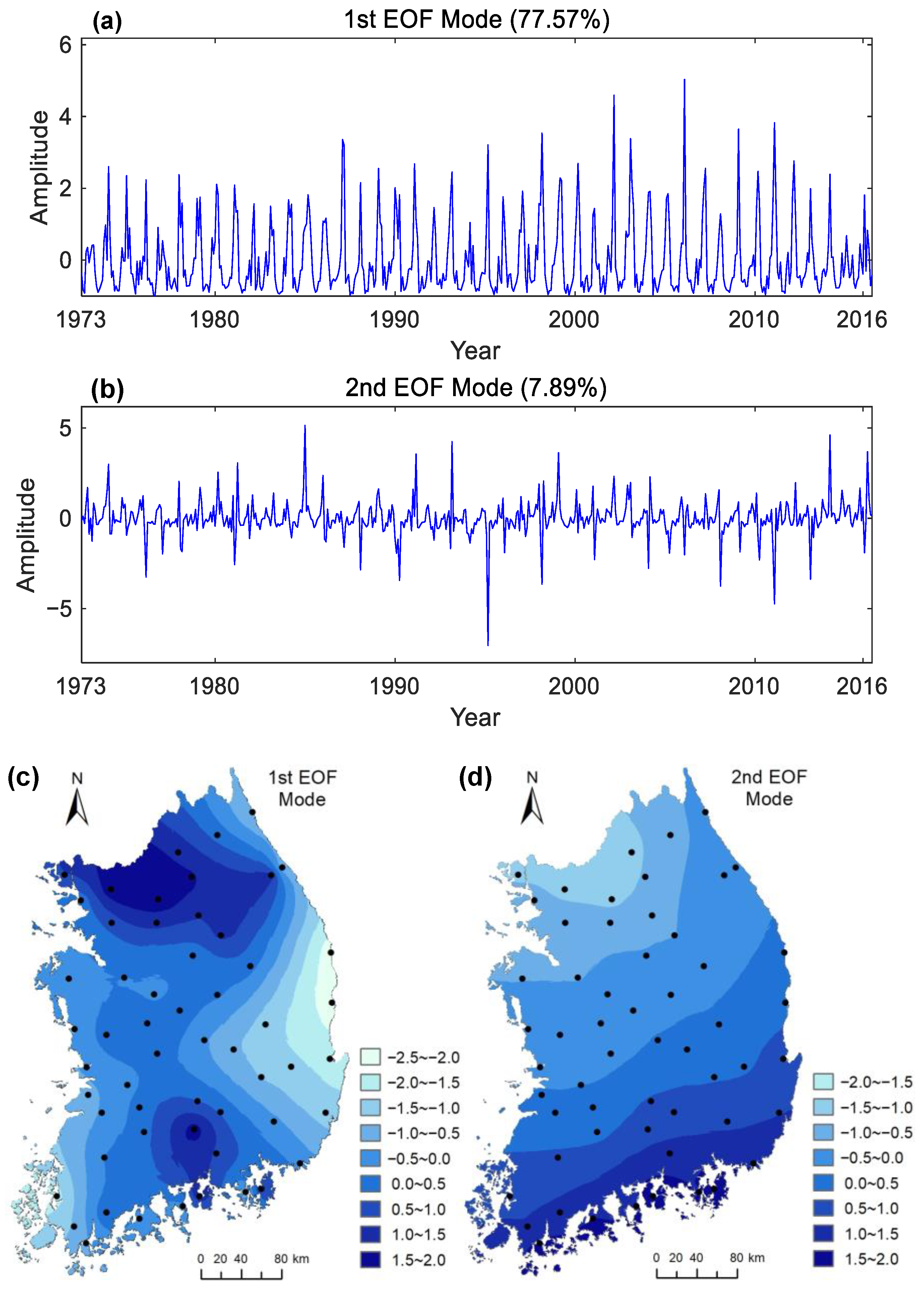
2.2.1. Empirical Orthogonal Function

Empirical orthogonal function analyses [30] are among the most widely applied techniques in oceanography and atmospheric science research. In this method, a spatiotemporal dataset is decomposed into orthogonal basis functions determined by the data. The method is similar to principal component analysis; however, EOFs can detect both temporal and spatial patterns.
In EOF analyses, spatiotemporal data X(r,t) are represented in terms of loading vectors (L) and their principal component (PC) time series, as follows:
X ( r , t ) = n P C n ( t ) L n ( r )
where Ln(r) represents a specific spatial pattern and PCn(t) represents the temporal evolution of Ln(r).
This equation signifies a decomposition of a given dataset into a number of spatial and temporal patterns. The spatial patterns are orthogonal to each other and are ordered by magnitude; the temporal patterns oscillate over time. The loading vectors represent the independent patterns of variability in the dataset and are often interpreted as a physical model of the system from which the data were derived [31].

2.2.2. Cyclostationary Empirical Orthogonal Function

A CSEOF is the basic function in a cyclostationary process and is a cyclostationary analog of an EOF obtained using a stationary approach [32]. The CSEOF analysis method is described in detail by Kim and North [33]. In CSEOF analyses, spatiotemporal data are represented as follows:
X ( r , t ) = k = 0 d 1 c k ( r , t ) e 2 π i k t / d
where d is the nested period representing the inherent periodicity in the data.
By calculating the covariance function and the Bloch function, the space–time CSEOFs can be obtained using the following equation:
X ( r , t ) = n P C n ( t ) C L n ( r , t )
where CLn(r,t) is a cyclostationary loading vector (CSLV) and PCn(t) is the corresponding PC time series.
In contrast to EOF analyses, the CSLVs are time-dependent. The temporal evolution of a spatial pattern also depends on periodic data with period d, calculated as follows:
C L n ( r , t ) = C L n ( r , t + d )
Thus, CSLVs are periodic, time-dependent eigenfunctions of the covariance statistics.
An essential component in CSEOF analyses is determining the nested period. Selecting a proper nested period requires an adequate understanding of the physical and statistical characteristics of the dataset being analyzed [34].
The CSEOF technique is conceptually similar to the EOF technique in that both extract sequences of spatial patterns as eigenfunctions based on the spatiotemporal structure of the covariance function. However, the major difference between EOF and CSEOF is that in CSEOF analyses, each CSLV represents a set of spatial patterns. The critical motivation for the temporal dependence of CSLVs is that the spatial patterns of many known phenomena in climate science and geophysics evolve over time with recognizable periods while exhibiting slow fluctuations over longer time scales. A comparison of studies that used EOF and CSEOF techniques can be found in Kim and Wu [35]. Recent studies have demonstrated the efficacy of CSEOFs in extracting robust modes representing climate variabilities [36,37].

2.2.3. Autoregressive Integrated Moving Average (ARIMA)

An autoregressive integrated moving average (ARIMA) was introduced by Box and Jenkins [38]. It is a statistical analysis model that uses time series data to either better understand the data set or to forecast future tendency. This model is usually applied to estimate related values in a time series; it is autoregressive if it predicts future values based on past values
An ARIMA(p,d,q) model can be understood by outlining each of its components as follows. Autoregression (AR): refers to a model that shows a changing variable that regresses on its own lagged, or prior, values. Integrated (I): represents the differencing of raw observations to allow for the time series to become stationary. Moving average (MA): incorporates the dependency between an observation and a residual error from a moving average model applied to lagged observations. Thus, the model can be written as follows:
( 1 i = 1 p α i L i ) ( 1 L ) d X t = ( 1 + j = 1 q β j L j ) ε t
where Xt is the time series value, p is order of the autoregressive part, d degree of first differencing involved, q is order of the moving average part, α and β are the parameters of the model, ε is white noise and L is Lag operator.
The key difficulty in applying the ARIMA model is identifying the orders of the model. Numerous available tests can be used to determine the orders of an ARIMA model. Two common proposed methods include the Akaike information criterion (AIC) and the Bayesian information criterion (BIC) [39,40].
The scheme of the forecasting approaches is shown in Figure 2.

3. Results and Discussion

3.1. Seasonal Cycle of Precipitation

The spatial distribution of mean precipitation in South Korea from 1973 to 2021 is shown in Figure 3, where the distribution represents the precipitation interpolation at each weather station. The means of precipitation in Figure 3 indicate the primary variabilities in precipitation. As expected, the mean is more in the north and south and less in the middle because of seasonal fluctuations in precipitation in the summer.
The annual precipitation is approximately 11,250 mm (1973–2021 average), with more than 60% of the annual rainfall occurring between June and August. Boxplots of the monthly precipitation from 1973 to 2021 are plotted in Figure 4. The annual periodicity involves obvious precipitation increases in the summer, with maximums occurring in July and August corresponding to the summer monsoon in Asia; precipitation is lower at other times of the year.
The precipitation data are decomposed into individual modes using EOF and CSEOF analyses. The main motivation for using these techniques is to investigate the mechanisms associated with changes in the variability of precipitation. A scree plot of the accumulated percentages obtained in the EOF and CSEOF analyses is shown in Figure 5 to show how they cumulatively rise. We present the two leading EOF and CSEOF modes to illustrate the temporal and spatial variations in precipitation.
Therefore, Figure 6 shows the first and second EOF modes, which explain 77.57% and 7.89% of the total variance, respectively. The PCs and loading patterns corresponding to the two leading modes are described in Figure 6a,b by normalized homogeneous correlation maps. The loading patterns in Figure 6c,d come from interpolation based on dispersion points.
The PC time series of the first and second modes of the EOF analysis (Figure 6a,b) both represent special cycles with slight fluctuations over longer time scales than those seen in the CSEOF modes. The amplitude of the first PC (Figure 6a) fluctuates over an annual cycle, similar to the original precipitation data. The loading patterns of the first EOF mode (Figure 6c) exhibit obvious symmetry between the north and south regions, and those of the second mode (Figure 6d) exhibit an increase from north to south.
The advantage of the CSEOF analysis is demonstrated by the PC time series. The nested period d is set to 12 months in the CSEOF analysis because the seasonal cycle is to be extracted. The first CSEOF mode of precipitation explains 73.86% of the total variance (Figure 7). The PC time series of the first mode (Figure 7a) and the cyclostationary loading patterns (Figure 7b) are shown for 12 months, from January to December. The loading patterns are interpolated based on the dispersion points. This mode denotes the seasonal cycle. The most pronounced feature of the CSLVs is the slowly varying precipitation throughout the year: the vectors indicate low rainfall from January to May, plenty of rainfall from June to September, and decreasing rainfall from October to December. The corresponding PC time series exhibits interannual and decadal variations in the seasonal cycle, as well as an increasing trend that is significant but not conspicuous, with stronger natural variability.
The second CSEOF mode shown in Figure 8 explains 5.05% of the total variance after omitting the seasonal cycle (the first mode) and adjusting for the seasonal cycle. The precipitation diminishes in April and then increases until July, decreases significantly in August and then increases until December. The PC time series of the second mode shows a positive phase shift in approximately 2006. Compared with the years before 2006, more recent precipitation tends to be more extensive. Thus, the second mode indicates slightly less precipitation in August and relatively large increases in precipitation in July.
In the EOF and CSEOF analyses, the thirteen leading EOF modes and fifteen leading CSEOF modes account for 95.15% and 95.22% of the total variance, respectively; these modes are statistically significant and distinct from the other modes; thus, they are selected for forecasting according to the rule of thumb [41]. The 13 leading temporal modes from the EOF and 15 modes form the CSEOF can account above 95% of total variance are interpreted as the primary conditions for the formation of precipitation, with the remaining modes considered as noise of data.

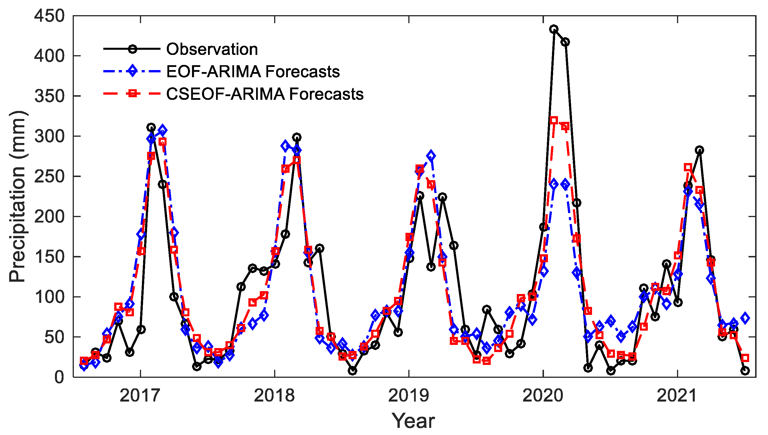
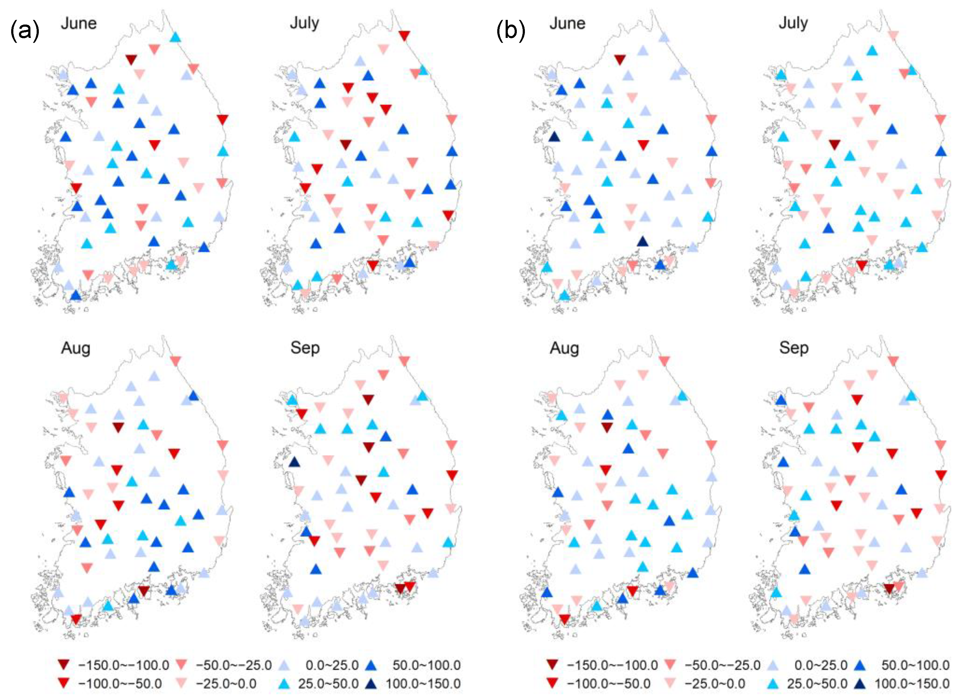
3.2. Forecasting of Precipitation

Once the precipitation data are decomposed into EOF and CSEOF modes, an ARIMA model is applied in the EOF and CSEOF space to derive precipitation variations in the PC time series. This composition of analysis and regression method results in two combined forecasting models: a combined EOF–ARIMA model and a combined CSEOF–ARIMA model.
Forecasts of the temporal patterns and timescales of the PCs can be estimated using these combined models. Figure 9 shows the forecasts for the four leading PCs of the precipitation data. The forecasts for the first PC obtained using the EOF–ARIMA model adequately capture the annual fluctuations, and the forecasts for the other PCs also exhibit cyclical fluctuations (Figure 9a) with smaller amplitudes. The forecasts obtained using the CSEOF–ARIMA model continue the interannual and decadal trends observed in the CSEOF analysis (Figure 9b). The amplitudes of the fluctuations are continuations of the past PCs; this is the goal of the CSEOF–ARIMA model.
Based on the PC forecasts, precipitation forecasts can be easily extrapolated using the loading vectors (spatial patterns) of the EOF and CSEOF. Quantitative precipitation forecasts are calculated for 56 weather stations over five years using the EOF–ARIMA and CSEOF–ARIMA models, and the results are then checked against the observed precipitation data. Figure 10 shows scatter plots of the observations and the forecasts resulting from the two models. The points corresponding to forecasts from EOF–ARIMA and observation partly dotted around above and below the y = x line divided by observation as 400 mm (Figure 10a). It means that the forecasts are slightly overestimated when less than 400 mm but underestimated when greater than 400 mm. In contrast, the points corresponding to forecasts from CSEOF–ARIMA and observation clustered around the y = x line (Figure 10b). It looks more evenly distributed and to have higher dispersion.
The mean monthly values of the precipitation forecasts obtained from the two combined models are compared with the observations, as shown in Figure 11. Because of the effect of the Asian monsoon, rainfall is uneven, with most rainfall occurring in the summer. The EOF–ARIMA forecasts are not particularly good, especially for the summer months. However, the CSEOF–ARIMA forecasts not only capture the seasonal variations in precipitation but also give confident quantitative predictions of the precipitation amounts.
The mean deviations of the forecasts obtained for the summer monsoon season (June, July, August and September) at each weather station are shown in Figure 12. The EOF–ARIMA model gives higher forecasts in June and September but relatively low forecasts in July and August (Figure 12a). In contrast, the mean deviation of the forecasts obtained from the CSEOF–ARIMA model are much smaller, with small overestimations in June and July and small underestimations in August and September (Figure 12b).
When the EOF method is used to analyze precipitation time series data, it cannot provide temporal variation responses in the spatial domain when decomposing the time components; thus, some errors result in the distribution analysis. The use of the CSEOF method can make up for this deficiency.
In the spatial distribution of the mean deviation (Figure 12a,b), the errors spread over in June are higher than those in July of the study area. We considered that the reason for this result is that precipitation increases obviously and the distribution changes greatly in July, leading to increased errors and causing the June and July deviation characteristics in both methods.
Several statistical measures are used to evaluate the performance of the forecasting methods: the mean absolute error (MAE), the root mean squared error (RMSE) and the coefficient of determination (R2). We use these standards to measure the error between the observed value and simulated value of our model so as to measure the applicability and practicability of our model as a whole. Table 1 provides a comparison of these measures applied for the two combined models. The results show that both models achieve good performance and that their accuracies are similar. However, the performance of the CSEOF–ARIMA model is better than that of the EOF–ARIMA model under every measure. The overall results indicate that the CSEOF–ARIMA model is an effective approach for precipitation forecasting.

4. Discussion

Many scholars have adopted a wide range of methods for studying the precipitation prediction work in South Korea, such as using the Weather Research and Forecasting (WRF) and Very-Short-Range Forecast of Precipitation (VSRF) system models for precipitation forecasting in individual basins of South Korea [42,43,44]. In addition, some academics focused on monthly precipitation forecasting over south Korea by combining the superensemble procedure with eigenvector analysis and correlation analysis [45,46]. Based on three different Bayesian Regression Models, other researchers investigated the precipitation forecasting of summer season in a region around Korea [47].
In order to better describe the performance of our model, we compare our model to the published research about precipitation forecasting in Korea. The results are shown in Table 2.
Table 2 shows the comparison between our model and several published characteristic models on their study area input, datasets, time scale period and performance evaluation.
From the table, we can see that the study areas of these models are all or part of South Korea, which provides comparability in this paper. In terms of data sources, the precipitation data used in each model were basically station, satellite and radar observation data. Data selection mainly depends on the characteristics and requirements of each model The SVDA and CSEOF models all used station data, and others used satellite and radar data. In the comparison of predictors, all models used some ocean variables as predictors except ours; our model used its own station data as a predictor. Therefore, our model is relatively simple in the composition architecture. From the analysis of time scale, the WRF model system could forecast precipitation on multiple hour scale, which is the advantage of these models. While other statistical models (include ours) could only do precipitation forecasting on monthly scale. In terms of time period, some models are only aimed at the forecast of concentrated rainfall in summer, while statistical models are aimed at the precipitation forecast of long-time series throughout the year. From the analysis of model performance, although there are differences in time scale, these models had obtained accurate and reliable results.
We can see that our model only uses its own data as input data and does not have as much data as other models. This is the characteristic of our model that is different from other models.
In our work, we provide a relatively simple method based on statistics for precipitation forecasting in South Korea. The required data are only the rainfall observation data of each station without complex data requirements. In terms of accuracy, it may not be more accurate than other complicated methods, but it has strong applicability and can be applied to station rainfall prediction in various or specific areas.

5. Conclusions

This study extends research and provides a simple and feasible method for precipitation forecasting that only relies on stations’ precipitation data. We investigated the spatiotemporal variability in precipitation data in South Korea using EOF and CSEOF analyses and proposed an effective methodology for precipitation forecasting. Of the total variance in the spatial distribution and temporal evolution of the studied precipitation data, the 13 leading EOF modes accounted for 95.15%, and the 15 leading CSEOF modes accounted for 95.22%. The EOF modes represented cycles with longer time scales than the CSEOF modes; the CSEOF modes represented interannual and decadal variations in the seasonal cycle with stronger natural variabilities than those seen in the EOF modes.
We estimated precipitation forecasts using a regression method. The PC forecasts obtained from the EOF–ARIMA model exhibited clear cyclical fluctuations, and those obtained from the CSEOF–ARIMA model represented extensions of the interannual and decadal variations observed in the CSEOF analysis. Based on the PC forecasts, quantitative precipitation forecasts were calculated for 56 stations over five years using the EOF–ARIMA and CSEOF–ARIMA models; these forecasts were then checked against the observed precipitation data.
In this article, we combined the EOF and CSEOF models with the ARIMA model, respectively, for precipitation forecasting. Based on the comparison between the simulated values of the two models and the observed values, through the statistical measured values (MAE, RMSE, R2), we preliminarily draw this conclusion: For these two models, the CSEOF–ARIMA combined model performed better than the EOF–ARIMA combined model. Because in the CSEOF analysis part, the precipitation data are decomposed into monthly spatial distribution. That means the CSEOF model can fully take into account the seasonal variation characteristics of rainfall data within the year, which shows the advantages over the EOF model.
The finding suggests that the combined CSEOF–ARIMA forecasting model gave the better approximation performance and that it captured the variational trends, temporal evolution and recurrent seasonal cycles in the precipitation data. These results indicate that the use of the CSEOF–ARIMA model is an accurate and efficient approach for precipitation forecasting in Korea.

Author Contributions

Conceptualization, M.S.; methodology, G.K. and Y.W.; validation and resources, M.S. and K.L. All authors have read and agreed to the published version of the manuscript.

Funding

This research was funded by Key Techniques for the Pollutant Source Apportionment and Water Quality Management and their application in the typical contaminated zone of Bohai Sea, grant number 2018YFC140707604.

Institutional Review Board Statement

Not applicable.

Informed Consent Statement

Not applicable.

Data Availability Statement

Not applicable.

Acknowledgments

We are thankful to all those who contributed to this study.

Conflicts of Interest

The authors declare no conflict of interest.

References

  1. Trenberth, K.E. Recent Observed Interdecadal Climate Changes in the Northern Hemisphere. Bull. Am. Meteorol. Soc. 1990, 71, 377–390. [Google Scholar] [CrossRef] [Green Version]
  2. Alijanian, M.; Rakhshandehroo, G.R.; Mishra, A.K.; Dehghani, M. Evaluation of satellite rainfall climatology using CMORPH, PERSIANN-CDR, PERSIANN, TRMM, MSWEP over Iran. Int. J. Climatol. 2017, 37, 4896–4914. [Google Scholar] [CrossRef]
  3. Yao, J.; Chen, Y.; Yu, X.; Zhao, Y.; Yang, L. Evaluation of multiple gridded precipitation datasets for the arid region of northwestern China. Atmos. Res. 2020, 236, 104818. [Google Scholar] [CrossRef]
  4. Huntington, T.G. Evidence for intensification of the global water cycle: Review and synthesis. J. Hydrol. 2006, 319, 83–95. [Google Scholar] [CrossRef]
  5. Oki, T.; Kanae, S. Global hydrological cycles and world water resources. Science 2006, 313, 1068–1072. [Google Scholar] [CrossRef] [Green Version]
  6. Nicholls, N.; Alexander, L. Has the climate become more variable or extreme? Progress 1992–2006. Prog. Phys. Geogr. 2007, 31, 77–87. [Google Scholar] [CrossRef]
  7. Becker, S.; Gemmer, M.; Jiang, T. Spatiotemporal analysis of precipitation trends in the Yangtze River catchment. Stoch. Environ. Res. Risk Assess. 2006, 20, 435–444. [Google Scholar] [CrossRef]
  8. Lim, Y.K.; Kim, K.Y. A New Perspective on the Climate Prediction of Asian Summer Monsoon Precipitation. J. Clim. 2006, 19, 4840–4853. [Google Scholar] [CrossRef]
  9. Zhou, B.T.; Wang, H. Relationship between the boreal spring Hadley circulation and the summer precipitation in the Yangtze River valley. J. Geophys. Res. Atmos. 2006, 111, 275. [Google Scholar] [CrossRef]
  10. Kim, J.; Miller, N.L.; Farrara, J.D.; Hong, S.Y. A Seasonal Precipitation and Stream Flow Hindcast and Prediction Study in the Western United States during the 1997/98 Winter Season Using a Dynamic Downscaling System. J. Hydrometeorol. 2000, 1, 311–329. [Google Scholar] [CrossRef]
  11. Higgins, R.W.; Kim, H.K.; Unger, D. Long-Lead Seasonal Temperature and Precipitation Prediction Using Tropical Pacific SST Consolidation Forecasts. J. Clim. 2004, 17, 3398–3414. [Google Scholar] [CrossRef]
  12. Wang, H.; Ting, M.; Ji, M. Prediction of seasonal mean United States precipitation based on El Niño sea surface temperatures. Geophys. Res. Lett. 1999, 26, 1341–1344. [Google Scholar] [CrossRef]
  13. Silverman, D.; Dracup, J.A. Artificial Neural Networks and Long-Range Precipitation Prediction in California. J. Appl. Meteor 2010, 39, 57–66. [Google Scholar] [CrossRef]
  14. Block, P.; Rajagopalan, B. Interannual Variability and Ensemble Forecast of Upper Blue Nile Basin Kiremt Season Precipitation. J. Hydrometeorol. 2007, 8, 327. [Google Scholar] [CrossRef] [Green Version]
  15. Peel, S.; Wilson, L.J. A Diagnostic Verification of the Precipitation Forecasts Produced by the Canadian Ensemble Prediction System. Weather. Forecast. 2008, 23, 1. [Google Scholar] [CrossRef]
  16. Chang, H.; Kwon, W.T. Spatial variations of summer precipitation trends in South Korea, 1973–2005. Environ. Res. Lett. 2007, 2, 45012–45019. [Google Scholar] [CrossRef] [Green Version]
  17. Jin, Y.H.; Kawamura, A.; Jinno, K.; Berndtsson, R. Detection of ENSO-influence on the monthly precipitation in South Korea. Hydrol. Processes 2005, 19, 4081–4092. [Google Scholar] [CrossRef]
  18. Kim, K.Y.; Kim, Y.Y. Investigation of tropical Pacific upper-ocean variability using cyclostationary EOFs of assimilated data. Ocean Dyn. 2004, 54, 489–505. [Google Scholar] [CrossRef] [Green Version]
  19. Wang, B.; Ding, Q.; Jhun, J.G. Trends in Seoul (1778–2004) summer precipitation. Geophys. Res. Lett. 2006, 33, 292–306. [Google Scholar] [CrossRef] [Green Version]
  20. Aghakouchak, A. Evaluation of satellite-retrieved extreme precipitation rates across the central United States. J. Geophys. Res. Atmos. 2011, 116, 1–11. [Google Scholar] [CrossRef]
  21. Stampoulis, D.; Anagnostou, E.N. Evaluation of Global Satellite Rainfall Products over Continental Europe. J. Hydrometeorol. 2012, 13, 588–603. [Google Scholar] [CrossRef]
  22. Gaona, M.; Overeem, A.; Brasjen, A.M.; Meirink, J.F.; Leijnse, H.; Uijlenhoet, R. Evaluation of Rainfall Products Derived From Satellites and Microwave Links for The Netherlands. IEEE Trans. Geosci. Remote Sens. 2017, 55, 6849–6859. [Google Scholar] [CrossRef]
  23. Barnston, A.G.; He, Y.; Glantz, M.H. Predictive Skill of Statistical and Dynamical Climate Models in SST Forecasts during the 1997–98 El Niño Episode and the 1998 La Niña Onset. Bull. Am. Meteorol. Soc. 1999, 80, 217–243. [Google Scholar] [CrossRef] [Green Version]
  24. Vautard, R.; Plaut, G.; Wang, R.; Brunet, G. Seasonal Prediction of North American Surface Air Temperatures Using Space-Time Principal Components. J. Clim. 1999, 12, 380–394. [Google Scholar] [CrossRef]
  25. Waliser, D.E.; Jones, C.; Schemm, J.K.E.; Graham, N.E. A Statistical Extended-Range Tropical Forecast Model Based on the Slow Evolution of the Madden-Julian Oscillation. J. Clim. 1999, 12, 1918–1939. [Google Scholar] [CrossRef] [Green Version]
  26. Waliser, D.E.; Lau, K.M.; Stern, W.; Jones, C. Potential Predictability of the Madden-Julian Oscillation. Bull. Am. Meteorol. Soc. 2003, 84, 33–50. [Google Scholar] [CrossRef] [Green Version]
  27. Cahalan, R.F.; Wharton, L.E.; Wu, M.L. Empirical orthogonal functions of monthly precipitation and temperature over the United States and homogeneous stochastic models. J. Geophys. Res. Atmos. 1996, 101, 26309–26318. [Google Scholar] [CrossRef]
  28. Singh, C.V. Empirical Orthogonal Function (EOF) analysis of monsoon rainfall and satellite-observed outgoing long-wave radiation for Indian monsoon: A comparative study. Meteorol. Atmos. Phys. 2004, 85, 227–234. [Google Scholar] [CrossRef]
  29. Svensson, C. Empirical Orthogonal Function Analysis of Daily Rainfall in the Upper Reaches of the Huai River Basin, China. Theor. Appl. Climatol. 1999, 62, 147–161. [Google Scholar] [CrossRef]
  30. Lorenz, E.N. Empirical Orthogonal Functions and Statistical Weather Prediction; Scientific Report No. 1; MIT: Cambridge, MA, USA, 1956; pp. 1–49. [Google Scholar]
  31. Hannachi, A.; Jolliffe, I.T.; Stephenson, D.B. Empirical orthogonal functions and related techniques in atmospheric science: A review. Int. J. Climatol. 2007, 27, 1119–1152. [Google Scholar] [CrossRef]
  32. Kim, K.; North, G.R.; Huang, J. EOFs of One-Dimensional Cyclostationary Time Series: Computations, Examples, and Stochastic Modeling. J. Atmos. Sci. 1996, 53, 1007–1017. [Google Scholar] [CrossRef] [Green Version]
  33. Kim, K.; North, G.R. EOFs of Harmonizable Cyclostationary Processes. J. Atmos. Sci. 1997, 54, 2416–2427. [Google Scholar] [CrossRef]
  34. Kim, K.; Chung, C. On the Evolution of the Annual Cycle in the Tropical Pacific. J. Clim. 2001, 14, 991–994. [Google Scholar] [CrossRef]
  35. Kim, K.; Wu, Q. A Comparison Study of EOF Techniques: Analysis of Nonstationary Data with Periodic Statistics. J. Clim. 1999, 12, 185–199. [Google Scholar] [CrossRef]
  36. Kim, K.; Roh, J. Physical Mechanisms of the Wintertime Surface Air Temperature Variability in South Korea and the near-7Day Oscillations. J. Clim. 2010, 23, 2197–2212. [Google Scholar] [CrossRef]
  37. Kim, Y.; Kim, K.-Y.; Kim, B.-M. Physical mechanisms of European winter snow cover variability and its relationship to the NAO. Clim. Dyn. 2013, 40, 1657–1669. [Google Scholar] [CrossRef]
  38. Box, G.E.P.; Jenkins, G.M. Time Series Analysis: Forecasting and Control; Holden-Day: San Francisco, CA, USA, 1971. [Google Scholar]
  39. Akaike, H. A New Look at the Statistical Model Identification. IEEE Trans. Autom. Control 1974, 19, 716–723. [Google Scholar] [CrossRef]
  40. Schwarz, G. Estimating the Dimension of a Model. Ann. Stat. 1978, 6, 461–464. [Google Scholar] [CrossRef]
  41. North, G.R.; Bell, T.L.; Cahalan, R.F.; Moeng, F.J. Sampling Errors in the Estimation of Empirical Orthogonal Functions. Mon. Weather Rev. 1982, 110, 699. [Google Scholar] [CrossRef]
  42. Jabbari, A.; So, J.-M.; Bae, D.-H. Precipitation Forecast Contribution Assessment in the Coupled Meteo-Hydrological Models. Atmosphere 2020, 11, 34. [Google Scholar] [CrossRef] [Green Version]
  43. Jee, J.B.; Ki, S. Sensitivity Study on High-Resolution WRF Precipitation Forecast for a Heavy Rainfall Event. Atmosphere 2017, 8, 96. [Google Scholar] [CrossRef] [Green Version]
  44. Kim, H.; Choi, J.; Nam, K.-Y.; Chang, K.; Oh, S. The Operational Very Short Range Forecast of Precipitation and its Hydrological Applications in South Korea. In Proceedings of the 33rd Conference on Radar Meteorology, Cairns, Australia, 5–10 August 2007. [Google Scholar]
  45. Kim, M.K.; Kang, I.S.; Park, C.K.; Kim, K.M. Superensemble prediction of regional precipitation over Korea. Int. J. Climatol. 2004, 24, 777–790. [Google Scholar] [CrossRef]
  46. Sun, M.; Kim, G. Quantitative Monthly Precipitation Forecasting Using Cyclostationary Empirical Orthogonal Function and Canonical Correlation Analysis. J. Hydrol. Eng. 2016, 21, 123–145. [Google Scholar] [CrossRef]
  47. Jo, S.; Lim, Y.; Lee, J.; Kang, H.S.; Oh, H.S. Bayesian regression model for seasonal forecast of precipitation over Korea. Asia-Pac. J. Atmos. Sci. 2012, 48, 205–212. [Google Scholar] [CrossRef]
Figure 1. Location of 56 precipitation stations in South Korea.
Atmosphere 13 00500 g001
Figure 2. Scheme of the analysis and forecasting.
Atmosphere 13 00500 g002
Figure 3. Spatial distribution of mean monthly precipitation data totals from 1973–2021 in South Korea.
Atmosphere 13 00500 g003
Figure 4. Boxplots of monthly precipitation data totals from 1973 to 2021 in South Korea. The upper and lower boundaries of each box indicate the upper and lower quartiles of the distribution; the median values are shown by the cross and line within the box, and the extreme upper data values are shown by dots above and below the box.
Atmosphere 13 00500 g004
Figure 5. The scree plot of the accumulated percentage of EOF and CSEOF analysis, with 13 leading modes from the EOF, 15 modes from the CSEOF can account for more than 95% of total variance.
Atmosphere 13 00500 g005
Figure 6. First and second EOF modes of precipitation: (a) principal component time series of 1st EOF mode, (b) principal component time series of 2nd EOF mode, (c) loading vectors of 1st EOF mode, (d) loading vectors of 2nd EOF mode.
Atmosphere 13 00500 g006
Figure 7. First CSEOF modes of precipitation: (a) principal component time series, (b) cyclostationary loading vectors (CSLV).
Atmosphere 13 00500 g007
Figure 8. Second CSEOF modes of precipitation: (a) principal component time series, (b) cyclostationary loading vectors (CSLV).
Atmosphere 13 00500 g008
Figure 9. Forecasts of principal component time series based on EOF and CSEOF analysis. (a) PC forecasts of EOF–ARIMA, (b) PC forecasts of CSEOF–ARIMA.
Atmosphere 13 00500 g009
Figure 10. Scatter plots on observation and forecasts of EOF–ARIMA and CSEOF–ARIMA: (a) EOF–ARIMA forecasts, (b) CSEOF–ARIMA forecasts.
Atmosphere 13 00500 g010
Figure 11. Temporal mean of observation with EOF–ARIMA and CSEOF–ARIMA forecasts.
Atmosphere 13 00500 g011
Figure 12. Mean deviation distribution of forecasts of EOF–ARIMA and CSEOF–ARIMA in June, July, August and September, (a) EOF–ARIMA forecasts mean deviation distribution, (b) CSEOF–ARIMA forecasts mean deviation distribution.
Atmosphere 13 00500 g012
Table 1. Quantitative statistical verification measures of forecasts.
IndexMAE (mm)RMSE (mm)R2CC
EOF–ARIMA57.8674.440.790.68
CSEOF–ARIMA49.4167.710.870.76
Table 2. Comparison of several precipitation forecasting models in Korea.
Model or SystemStudy AreaPrecipitation Source TypePredictorTime ScaleTime PeriodPerformance Evaluation
RMSECCR2
Bayesian Regression Models [47]Over South KoreaStations and GridsGDAPSMonthly (Average JJA)1979–20071.09--
Meteorological Model of WRF [42]Imjin River Basin of Korea peninsulaStations and Grids-6 h2007–201159.67–212.80--
WRF Model [43]Seoul & suburban in South KoreaGridsSST Data3 h26–29 July 20112.54–13.180.2–0.59-
VSRF model [44]Kyoungan River basin of South KoreaStations and Radar Reflectivity-Hourly 5.77–7.67-0.7–0.8
SVDA and CCA [45]Over South KoreaStationsSLP DataMonthly1954–2003-0.11–0.87-
Cyclostationary EOF and CCA [46]Over South KoreaStationsSSTMonthly1973–201354.17–63.850.69–0.730.55–0.67
Cyclostationary EOF and ARIMAOver South KoreaStationsPrecipitationMonthly1973–202167.71–74.440.79–0.870.68–0.76
Publisher’s Note: MDPI stays neutral with regard to jurisdictional claims in published maps and institutional affiliations.

