
The Relationship between PM2.5 and PM10 in Central Italy: Application of Machine Learning Model to Segregate Anthropogenic from Natural Sources

 , , and
Abstract
:1. Introduction
2. Methodology
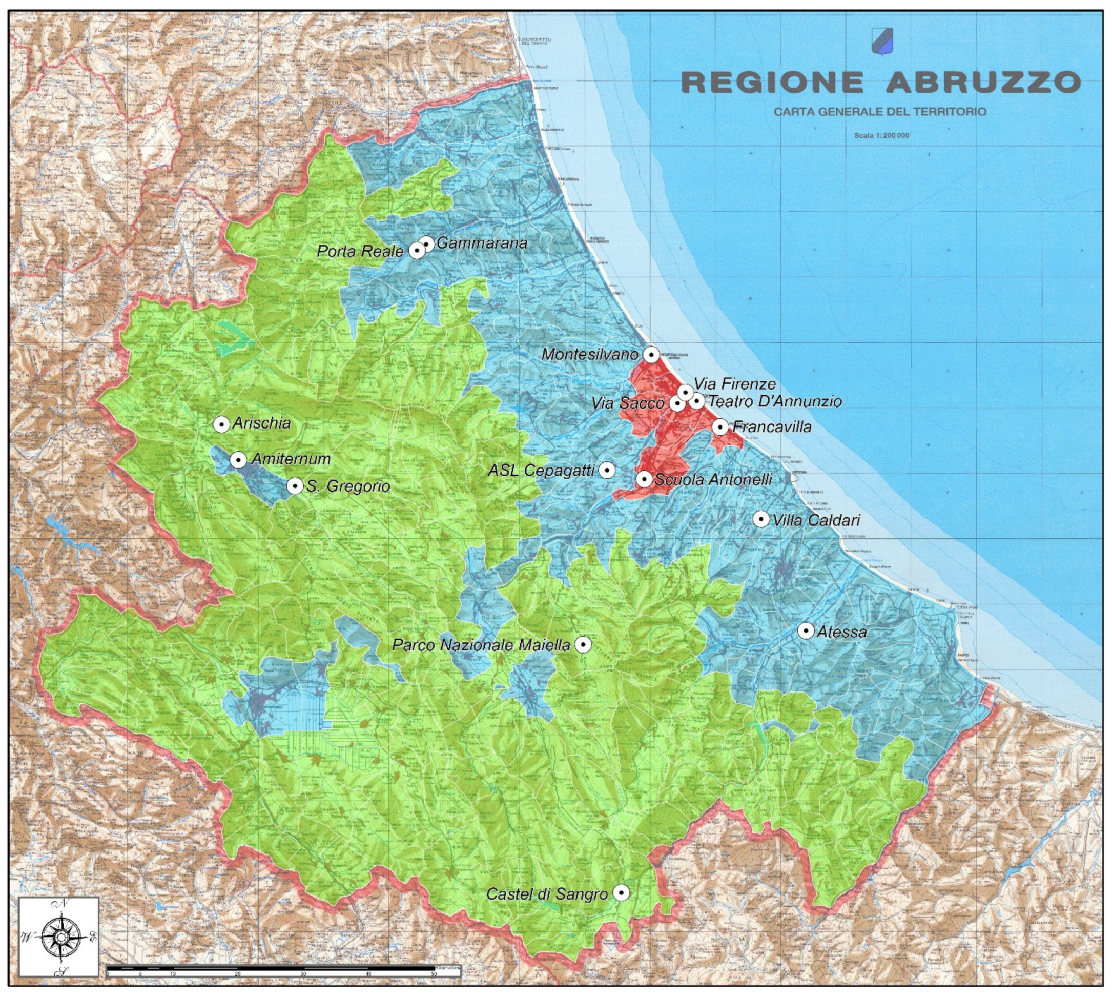
2.1. Study Area
2.2. Model Analysis
2.3. Sampling and Data Analysis
2.4. Lin and Pearson Coefficient
3. Results and Discussion
4. Conclusions
Author Contributions
Funding
Institutional Review Board Statement
Informed Consent Statement
Data Availability Statement
Acknowledgments
Conflicts of Interest
References
- Liu, Y.; Zhou, Y.; Lu, J. Exploring the relationship between air pollution and meteorological conditions in China under environmental governance. Nat. Res. Sci. Rep. 2020, 10, 14518. [Google Scholar] [CrossRef] [PubMed]
- Kayes, I.; Shahriar, S.A.; Hasan, K.; Akhter, M.; Kabir, M.M.; Sala, M.A. The relationships between meteorological parameters and air pollutants in an urban environment Global. J. Environ. Sci. Manag. 2019, 5, 265–278. [Google Scholar]
- Li, C.; Huang, Y.; Guo, H.; Wu, G.; Wang, Y.; Li, W.; Cui, L. The Concentrations and Removal Effects of PM10 and PM2.5 on a Wetland in Beijing. Sustainability 2019, 11, 1312. [Google Scholar] [CrossRef] [Green Version]
- Arhami, M.; Kamali, N.; Rajabi, M.M. Predicting hourly air pollutant levels using artificial neural networks coupled with uncertainty analysis by Monte Carlo simulations. Environ. Sci. Pollut. 2013, 20, 4777–4789. [Google Scholar] [CrossRef] [PubMed]
- Biancofiore, F.; Verdecchia, M.; Di Carlo, P.; Tomassetti, B.; Aruffo, E.; Busilacchio, M.; Bianco, S.; Di Tommaso, S.; Colangeli, C. Analysis of surface ozone using a recurrent neural network. Sci. Total Environ. 2015, 514, 379–387. [Google Scholar] [CrossRef] [PubMed]
- Biancofiore, F.; Busilacchio, M.; Verdecchia, M.; Tomassetti, B.; Aruffo, E.; Bianco, S.; Di Tommaso, S.; Colangeli, C.; Rosatelli, G.; Di Carlo, P. Recursive neural network model for analysis and forecast of PM10 and PM2.5. Atmos. Pollut. Res. 2017, 8, 652–659. [Google Scholar] [CrossRef]
- Aruffo, E.; Di Carlo, P.; Cristofanelli, P.; Bonasoni, P. Neural Network Model Analysis for Investigation of NO Origin in a High Mountain Site. Atmosphere 2020, 11, 173. [Google Scholar] [CrossRef] [Green Version]
- Chen, J.; De Hoogh, K.; Gulliverd, J.; Ho-Manne, B.; Hertelf, O.; Ketzel, M.; Bauwelinckh, M.; van Donkelaari, A.; Hvidtfeldtj, U.A.; Katsouyannik, K. Comparison of linear regression, regularization, and machine learning algorithms to develop Europe-wide spatial models of fine particles and nitrogen dioxide. Environ. Int. 2019, 130, 104934. [Google Scholar] [CrossRef] [PubMed]
- Cortina-Januchs, M.G.; Quintanilla-Dominguez, J.; Vega-Corona, A.; Andina, D. Development of a model for forecasting of PM10 concentrations in Salamanca, Mexico. Atmos. Pollut. Res. 2015, 10, 5094. [Google Scholar]
- Gardner, M.W.; Dorling, S.R. Neural network modeling and prediction of hourly NOx and NO2 concentrations in urban air in London. Atmos. Environ. 1999, 33, 709–719. [Google Scholar] [CrossRef]
- Mclean Cabanerosa, S.; Calautitb, J.K.; Hughesa, B.R. A review of artificial neural network models for ambient air pollution prediction. Environ. Model. Softw. 2019, 119, 285–304. [Google Scholar] [CrossRef]
- Grimes, D.I.F.; Coppola, E.; Verdecchia, M.; Visconti, G. A neural network approach to real-time rainfall estimation for Africa using satellite data. J. Hydrometeorol. 2003, 4, 1119–1133. [Google Scholar] [CrossRef]
- Shahraiyni, H.T.; Sodoudi, S. Statistical Modeling Approaches for PM10 Prediction in Urban Areas; A Review of 21st-Century Studies. Atmosphere 2016, 2, 15. [Google Scholar] [CrossRef] [Green Version]
- Abdullah, S.; Ismail, M.; Ahmed, A.N.; Abdullah, A.M. Forecasting Particulate Matter Concentration Using Linear and Non-Linear Approaches for Air Quality Decision Support. Atmosphere 2019, 10, 667. [Google Scholar] [CrossRef] [Green Version]
- May Tzuc, O.; Bassam, A.; Ricalde, L.J.; Cruz May, E. Sensitivity Analysis With Artificial Neural Networks for Operation of Photovoltaic Systems. In Artificial Neural Networks for Engineering Applications; Alanis, A.Y., Arana-Daniel, N., López-Franco, C., Eds.; Academic Press: Cambridge, MA, USA, 2019; Volume 10, pp. 127–138. [Google Scholar]
- Sairamya, N.J.; Susmitha, L.; Thomas George, S.; Subathra, M.S.P. Hybrid Approach for Classification of Electroencephalographic Signals Using Time-Frequency Images With Wavelets and Texture Features. In Intelligent Data Analysis for Biomedical Applications; Hemanth, D.J., Gupta, D., Balas, V.E., Eds.; Academic Press: Cambridge, MA, USA, 2019; Volume 12, pp. 253–273. [Google Scholar]
- Castro, W.; Oblitas, J.; Santa-Cruz, R.; Avila-George, H. Multilayer perceptron architecture optimization using parallel computing techniques. PLoS ONE 2017, 12, 0189369. [Google Scholar] [CrossRef] [PubMed] [Green Version]
- Guo, Z.; Chai, Q.; Maskell, D.L. FCMAC-AARS: A Novel FNN Architecture for Stock Market Prediction and Trading. In Proceedings of the IEEE International Conference on Evolutionary Computation, Vancouver, BC, Canada, 16–21 July 2006; pp. 2375–2381. [Google Scholar]
- Cattani, G.; Di Menno Di Bucchianico, A.; Gaeta, A.; Gandolfo, G.; Leone, G. Qualità dell’ambiente urbano. XIV Rapporto ISPRA Stato dell’Ambiente 82/18. Riv. Ital. di Econ. Demogr. e Stat. 2018, 5, 375–441. Available online: https://www.isprambiente.gov.it/it/pubblicazioni/stato-dellambiente/xiv-rapporto-qualita-dell2019ambiente-urbano-edizione-2018 (accessed on 20 January 2022).
- Zauli Sajani, S.; Scotto, F.; Lauriola, P.; Galassi, F.; Montanari, A. Urban Air Pollution Monitoring and Correlation Properties between Fixed-Site Stations. J. Air Waste Manag. Assoc. 1994, 54, 1236–1241. [Google Scholar] [CrossRef] [PubMed] [Green Version]
- Biggeri, A.; Baccini, M.; Accetta, G.; Bellini, A.; Grechi, D. Valutazione di qualità delle misure di concentrazione degli inquinanti atmosferici nello studio dell’effetto a breve termine dell’inquinamento sulla salute. Epidemiol. Prev. 2003, 27, 365–375. [Google Scholar] [PubMed]
- Palermi, S.; Polidoro, M.; Di Tommaso, S.; Colangeli, C.; Bianco, S. Omogeneità spaziale delle concentrazioni di Benzo(a)Pirene misurate presso due stazioni nell’area urbana di Pescara. Boll. Degli Esperti Ambient. 2016, 3, 45–58. [Google Scholar]
- Lawrence, I.; Lin, K. A Concordance Correlation Coefficient to Evaluate Reproducibility. Biometrics 1989, 45, 255–268. [Google Scholar]


| Area | Municipality | Station Name | Station ID | Latitude | Longitude | Type | PM10 | PM2.5 |
|---|---|---|---|---|---|---|---|---|
| Agglomerate Chieti-Pescara (AGG) | Pescara | T.D’annunzio | TH | N 4,700,733 m | E 437,102 m | UB | X | X |
| Pescara | Via Sacco | SA | N 4,700,366 m | E 434,150 m | UB | X | ||
| Pescara | Via Firenze | FI | N 4,702,020 m | E 435,376 m | UT | X | X | |
| Montesilvano | Montesilvano | MO | N 4,707,801 m | E 430,126 m | UT | X | X | |
| Chieti Scalo | Scuola Antonelli | CH | N 4,688,783 m | E 429,050 m | UB | X | X | |
| Francavilla al Mare | Francavilla | FR | N 4,697,015 m | E 429,050 m | UB | X | X | |
| Greater Anthropic Pressure (MAXP) | L’aquila | Amiternum | AQ | N 4,691,713 m | E 366,938 m | UB | X | X |
| L’aquila | S. Gregorio | SG | N 4,687,738 m | E 375,604 m | SB | |||
| Teramo | Gammanara | GA | N 4,724,660 m | E 395,690 m | UB | X | ||
| Teramo | Porta Reale | PR | N 4,723,748 m | E 394,297 m | UT | X | ||
| Cepagatti | ASL Cepagatti | CE | N 460,147 m | E 423,332 m | RB | |||
| Ortona | Villa Caldari | OR | N 4,682,708 m | E 446,950 m | SB | X | X | |
| Atessa | Atessa | AT | N 4,665,673 m | E 453,840 m | I | X | ||
| Lower Anthropic Pressure (minp) | Castel di Sagro | Castel di Sangro | CS | N 4,625,609 m | E 425,526 m | SB | X | X |
| Arischia | Arischia | AR | N 4,697,123 m | E 364,389 m | RB | |||
| S. Eufemia A Majella | Parco Nazionale Maiella | PNM | N 4,663,534 m | E 419,701 m | RB |
| Period | Statistic | TH | FI | MO | CH | FR | OR | AQ | CS |
|---|---|---|---|---|---|---|---|---|---|
| winter sem. | mean | 20.2 | 19.7 | 20.0 | 20.5 | 16.2 | 14.5 | 12.9 | 9.2 |
| median | 18 | 18 | 18 | 19 | 14 | 13 | 12 | 9 | |
| st.dev. | 11.8 | 10.7 | 9.4 | 10.9 | 9.1 | 8.1 | 7.1 | 4.6 | |
| min | 3 | 3 | 3 | 3 | 3 | 2 | 2 | 1 | |
| max | 59 | 50 | 47 | 53 | 43 | 46 | 43 | 29 | |
| summer sem. | mean | 11.5 | 11.9 | 11.9 | 11.9 | 10.3 | 11.0 | 9.3 | 8.5 |
| median | 11 | 12 | 12 | 12 | 10 | 11 | 9 | 8 | |
| st.dev. | 4.1 | 4.2 | 3.8 | 4.4 | 4.1 | 4.4 | 4.0 | 3.9 | |
| min | 3 | 4 | 4 | 4 | 3 | 2 | 2 | 2 | |
| max | 31 | 30 | 27 | 29 | 28 | 25 | 45 | 30 | |
| year | mean | 15.9 | 15.8 | 15.9 | 16.3 | 13.2 | 12.7 | 11.1 | 8.8 |
| median | 13 | 13 | 14 | 14 | 11 | 12 | 10 | 8 | |
| st.dev. | 9.9 | 9.0 | 8.2 | 9.4 | 7.6 | 6.7 | 6.0 | 4.3 | |
| min | 3 | 3 | 3 | 3 | 3 | 2 | 2 | 1 | |
| max | 59 | 50 | 47 | 53 | 43 | 46 | 43 | 45 | |
| data av% | 95.1 | 97.0 | 96.3 | 91.1 | 96.7 | 96.0 | 97.9 | 91.9 |
| Period | Statistic | TH | FI | MO | CH | FR | OR | AQ | CS |
|---|---|---|---|---|---|---|---|---|---|
| winter sem. | mean | 28.1 | 28.4 | 28.2 | 26.8 | 21.7 | 19.0 | 18.4 | 12.7 |
| median | 27 | 27 | 27 | 26 | 20 | 17 | 18 | 12 | |
| st.dev. | 12.6 | 12.4 | 11.2 | 13.0 | 10.0 | 9.6 | 9.0 | 6.2 | |
| min | 6 | 6 | 7 | 5 | 6 | 4 | 3 | 2 | |
| max | 65 | 65 | 68 | 80 | 62 | 53 | 47 | 38 | |
| summer sem. | mean | 23.7 | 20.8 | 20.3 | 19.1 | 17.7 | 17.0 | 15.3 | 13.4 |
| median | 23 | 20 | 20 | 18 | 17 | 16 | 14 | 12 | |
| st.dev. | 8.7 | 6.5 | 6.0 | 6.8 | 6.3 | 7.0 | 6.9 | 6.8 | |
| min | 5 | 6 | 6 | 7 | 5 | 4 | 4 | 4 | |
| max | 86 | 48 | 46 | 53 | 64 | 61 | 58 | 60 | |
| year | mean | 25.9 | 24.6 | 24.3 | 23.1 | 19.7 | 18.0 | 16.8 | 13.1 |
| median | 24 | 22 | 22 | 21 | 18 | 16.5 | 13 | 12 | |
| st.dev. | 10.8 | 10.4 | 9.6 | 10.9 | 8.4 | 8.3 | 8.0 | 6.5 | |
| min | 5 | 6 | 6 | 5 | 5 | 4 | 3 | 2 | |
| max | 86 | 65 | 68 | 80 | 64 | 61 | 58 | 60 | |
| data av% | 94.8 | 96.9 | 96.9 | 92.5 | 97.1 | 96.0 | 98.1 | 91.5 |
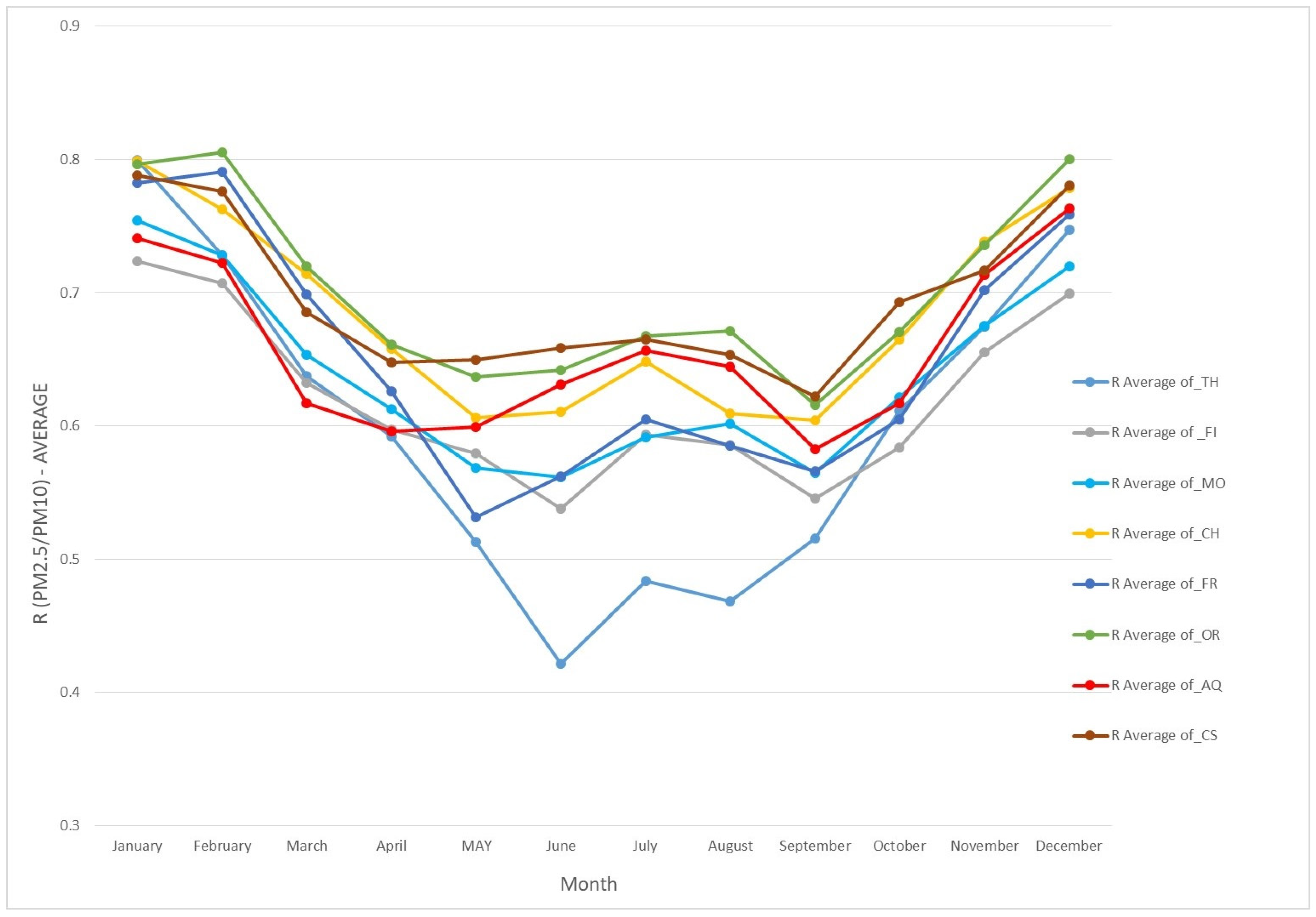
| Period | TH | FI | MO | CH | FR | OR | AQ | CS |
|---|---|---|---|---|---|---|---|---|
| April–September | 0.50 | 0.57 | 0.58 | 0.62 | 0.58 | 0.65 | 0.62 | 0.65 |
| October–March | 0.70 | 0.67 | 0.69 | 0.74 | 0.72 | 0.75 | 0.69 | 0.74 |
| year | 0.60 | 0.62 | 0.64 | 0.66 | 0.65 | 0.70 | 0.66 | 0.69 |
| PM2.5 | TH | FI | MO | CH | FR | OR |
|---|---|---|---|---|---|---|
| TH | 0.934 | 0.904 | 0.857 | 0.922 | 0.872 | |
| FI | 0.953 | 0.954 | 0.902 | 0.926 | 0.902 | |
| MO | 0.885 | 0.943 | 0.882 | 0.925 | 0.898 | |
| CH | 0.923 | 0.913 | 0.847 | 0.874 | 0.875 | |
| FR | 0.930 | 0.948 | 0.912 | 0.905 | 0.891 | |
| OR | 0.851 | 0.893 | 0.847 | 0.883 | 0.914 |
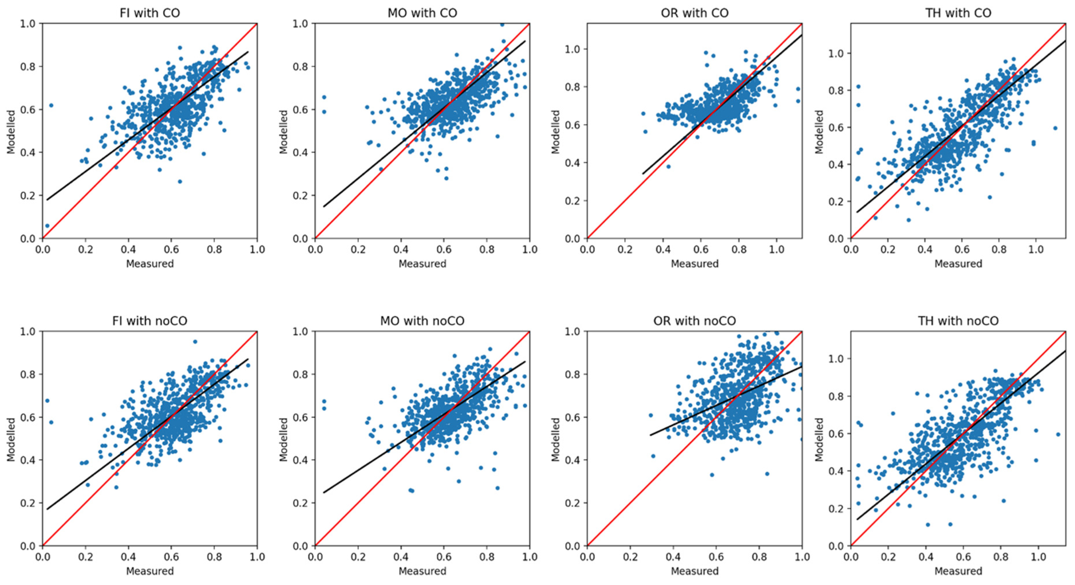
| CO | ||||||
|---|---|---|---|---|---|---|
| Station | R | NMSE | FB | FA2 | Slope | Intercept |
| CS | 0.45 | 0.04 | 0.02 | 1.03 | 0.58 | 0.30 |
| FI | 0.63 | 0.03 | 0.00 | 1.01 | 0.74 | 0.16 |
| MO | 0.57 | 0.03 | 0.00 | 1.01 | 0.82 | 0.11 |
| OR | 0.55 | 0.02 | −0.01 | 0.99 | 0.87 | 0.08 |
| TH | 0.74 | 0.05 | 0.02 | 1.02 | 0.82 | 0.11 |
| noCO | ||||||
| Station | R | NMSE | FB | FA2 | Slope | Intercept |
| CS | 0.36 | 0.04 | 0.02 | 1.03 | 0.60 | 0.28 |
| FI | 0.60 | 0.03 | 0.00 | 1.01 | 0.75 | 0.15 |
| MO | 0.51 | 0.03 | 0.00 | 1.01 | 0.65 | 0.22 |
| OR | 0.44 | 0.03 | 0.00 | 1.01 | 0.45 | 0.38 |
| TH | 0.70 | 0.06 | 0.00 | 1.03 | 0.81 | 0.11 |
| PM2.5 | FI-MO | MO-FR | FI-TH | FI-FR | TH-FR | TH-MO | TH-CH | CH-OR | TH-OR |
|---|---|---|---|---|---|---|---|---|---|
| April–September | 0.951 | 0.857 | 0.930 | 0.862 | 0.884 | 0.899 | 0.851 | 0.855 | 0.863 |
| October–March | 0.934 | 0.841 | 0.947 | 0.879 | 0.836 | 0.861 | 0.919 | 0.708 | 0.685 |
Publisher’s Note: MDPI stays neutral with regard to jurisdictional claims in published maps and institutional affiliations. |
© 2022 by the authors. Licensee MDPI, Basel, Switzerland. This article is an open access article distributed under the terms and conditions of the Creative Commons Attribution (CC BY) license (https://creativecommons.org/licenses/by/4.0/).
Share and Cite
Colangeli, C.; Palermi, S.; Bianco, S.; Aruffo, E.; Chiacchiaretta, P.; Di Carlo, P. The Relationship between PM2.5 and PM10 in Central Italy: Application of Machine Learning Model to Segregate Anthropogenic from Natural Sources. Atmosphere 2022, 13, 484. https://doi.org/10.3390/atmos13030484
Colangeli C, Palermi S, Bianco S, Aruffo E, Chiacchiaretta P, Di Carlo P. The Relationship between PM2.5 and PM10 in Central Italy: Application of Machine Learning Model to Segregate Anthropogenic from Natural Sources. Atmosphere. 2022; 13(3):484. https://doi.org/10.3390/atmos13030484
Chicago/Turabian StyleColangeli, Carlo, Sergio Palermi, Sebastiano Bianco, Eleonora Aruffo, Piero Chiacchiaretta, and Piero Di Carlo. 2022. "The Relationship between PM2.5 and PM10 in Central Italy: Application of Machine Learning Model to Segregate Anthropogenic from Natural Sources" Atmosphere 13, no. 3: 484. https://doi.org/10.3390/atmos13030484