Regional VOCs Gathering Situation Intelligent Sensing Method Based on Spatial-Temporal Feature Selection

Abstract

As VOCs pose a threat to human health, it is important to accurately capture changes in VOCs concentrations and sense VOCs concentrations in relevant areas. Therefore, it is necessary to improve the accuracy of VOCs concentration prediction and realise the VOCs aggregation situation sensing. Firstly, on the basis of regional grid division, the inverse distance spatial interpolation method is used for spatial interpolation to collect regional VOCs data information. Secondly, extreme gradient boosting (XGBoost) is used for spatio-temporal feature selection, combined with graph convolutional neural network (GCN) to construct regional spatial relationships of VOCs, and multiple linear regression (MLR) to process VOCs time series data and predict the VOCs concentration in the grid. Finally, the aggregation potential values of VOCs are calculated based on the prediction results, and the potential perception results are visualised. A VOCs aggregation perception method based on concentration prediction is proposed, using the XGBoost-GCN-MLR method with a scenario-aware approach for VOCs to perceive the VOCs aggregation in the relevant region. VOCs concentration prediction and VOCs aggregation trend perception were carried out in Xi’an, Baoji, Tongchuan, Weinan and Xianyang. The results show that compared with the GCN model, XGBoost model, MLR model and GCN-MLR model, the XGBoost-GCN-MLR model reduces the input variables, achieves the optimisation of the input parameters of the VOCs concentration prediction model, reduces the complexity of the prediction model and improves the prediction accuracy. Intelligent sensing of VOCs aggregation can visualise the regional VOCs. The intelligent sensing of VOCs aggregation can visualise the development trend and status of regional VOCs aggregation and convey more information, which has practical value.

1. Introduction

VOCs are very important trace components in the atmospheric troposphere and can react photochemically with nitrogen oxides (NOX) under ultraviolet light irradiation conditions and are important precursors to ozone (O₃) and fine particulate matter (PM_2.5). VOCs have a significant impact on the formation of secondary organic matter, ozone pollution [1]. In terms of human health risks, there may be a risk of cancer in people exposed to VOCs for long periods of time [2]. For example, VOCs are potentially carcinogenic, teratogenic, mutagenic and cause other adverse health effects in various organs and systems of the human body [3,4,5]. VOCs can cause chronic or acute damage to the human respiratory, haematopoietic and nervous systems, and may even induce symptoms such as asthma [6] and leukaemia [7]. VOCs are an important cause of increased concentrations of pollutants such as ozone in the atmosphere and their conversion to secondary organic particulate matter and ultimately to PM_2.5 [8]. In this aspect of environmental pollution, the emission of VOCs in the environment is characterised by regional aggregation. The migration of VOCs is temperature dependent, the higher the temperature, the higher the migration rate of VOCs [9]. When air pollution is severe and PM₁₀ and PM_2.5 concentrations are high, VOCs concentrations are also high. This means that when meteorological conditions are unfavourable for dispersion, atmospheric VOCs also accumulate and are not dispersed, resulting in peak concentrations. Higher concentrations of VOCs are more likely to form organic aerosols under certain conditions, resulting in more fine particles and increased atmospheric pollution [10]. Unreasonable emissions of pollutants have led to unusually high levels of air pollution, and the air pollution situation is becoming increasingly serious [11,12]. By predicting trends in VOCs concentrations and sensing the aggregation of VOCs in associated areas, it helps to capture the regional variation process of VOCS in time and space. This paper attempts to simulate the distribution of VOCs clustering potential in an attempt to better understand the trend and status of regional VOCs clustering and to promote the management of regional environmental conditions and pollution early warning. VOCs aggregation sensing can provide theoretical support to government departments in formulating air pollution control policies and pollutant reduction countermeasures and is of great significance in combating environmental pollution and safeguarding public health.

Many scholars are currently conducting research on the prediction of VOCs concentrations and they have used machine learning algorithms and deep learning algorithms to predict the changes in VOCs concentrations. Zhang et al. used a typical machine learning approach to predict the emission behaviour of furniture VOCs using artificial neural networks (ANN) [13]. Nkeshita et al. used ANN to predict the potential of total volatile organic compounds (TVOCs) released from local food waste decomposition [14]. Zhang utilised a deep neural network regression prediction model to achieve multi-component VOCs concentration inversion [15]. Ren et al. developed a prediction model for VOCs in industrial parks based on genetic algorithm and BP neural network [16]. Zhao applied the extreme learning machine (ELM) method to predict the concentration of each component in a mixed gas sample with four components fixed [17]. Chen provided BP neural network output nodes to give continuous prediction of the concentration of each VOC in the target analytes and to complete the quantitative analysis of the VOC gas mixture components within a certain error range [18]. Many scholars are currently conducting research on the prediction of VOCs concentrations and they have used machine learning algorithms and deep learning algorithms to predict the changes in VOCS concentrations. Compared to traditional BP neural network algorithms, the ELM method has the advantage of faster learning. However, in terms of factors influencing VOCS, these prediction studies have not been able to take into account the influence of meteorological factors on the variability of VOCS. In terms of VOCs study areas, these studies also focus on small regional sample data and do not predict VOCs aggregation in the region, while lacking a gridded, fine-scale study to get a sense of VOCs aggregation dynamics. In terms of prediction models for VOCs, these studies still lack the exploration of optimal combinations of prediction models, and the prediction accuracy needs to be improved.

More machine learning algorithms and deep learning algorithms are being used in the study of atmospheric pollutants, which brings more references to carry out trend prediction and aggregation sensing of VOCs, such as k-nearest neighbour (KNN) [19], random forest (RF) [20], multilayer perceptron (MLP) [21], long short-term memory (LSTM) [22,23], convolutional neural networks (CNN) [24] and chemical transport models (CTMs) [25]. PM_2.5, PM₁₀, O₃, NO₂, SO₂ and CO have more research results as common air pollutants. Al-Qaness et al. showed an improved version of the Adaptive Neuro-Fuzzy Inference System (ANFIS) to predict the air quality index in Wuhan, China [26]. Prihatno et al. developed a single dense layer bi-directional long and short-term memory (BiLSTM) model to predict PM_2.5 concentrations in indoor environments using time series data [27]. Guo et al. suggested a hybrid decomposition-integrated learning paradigm for PM_2.5 prediction based on variational pattern decomposition (VMD) and an improved whale optimisation algorithm (IWOA) [28]. Huang et al. developed an empirical modal decomposition (EMD-GRU) based gated recurrent unit neural network integration method for predicting PM_2.5 concentrations [29]. Photphanloet et al. presented a new model for predicting PM₁₀ concentrations based on a combination of a genetic algorithm, MLP and an improved depth-first search algorithm [30]. Durao et al. combined meteorological, air quality and industrial emissions data to predict O₃ levels in the Portuguese region through classification and regression trees combined with a multilayer perceptron model [31]. Liu et al. used an autoregressive integrated moving average (ARIMA) numerical forecasting model (ARIMAX) to predict air pollutants such as NO₂ [32]. Zhu et al. developed a support vector regression (SVR) model combined with the cuckoo search algorithm (CS) and the grey wolf optimisation algorithm (GWO) to model high and low frequency sequences to predict NO₂ or SO₂ in central China [33]. Nourani et al. produced an effective model using ANN and ANFIS to predict CO pollutant concentrations [34]. Wong et al. combined the Land Use Regression (LUR) model with XGBoost to predict PM_2.5 concentrations in Taiwan [35]. Just et al. applied the XGBoost model for recursive feature selection to predict daily PM_2.5 concentrations in 13 northeastern US states from 2000–2015 [36]. Muthukum et al. used GCN and convolutional long and short-term memory (ConvLSTM) to learn the spatial and temporal characteristics of PM_2.5 and predicted PM_2.5 concentrations in Los Angeles using meteorological data and ground-based observations and remote sensing satellite big data [37]. Qi et al. proposed a hybrid GCN and LSTM-based model (GC-LSTM) to model and predict the spatial and temporal variation in PM_2.5 concentrations [38]. Ren et al. developed and applied a daily average PM_2.5 prediction model for northern China by combining back propagation artificial neural network (BPANN) and MLR [39]. Kim et al. used aerosol optical depth (AOD) values from ground-based and satellite remote sensing observations to estimate PM_2.5 in Seoul based on the MLR model [40]. Studies related to these atmospheric pollutants have shown that effective meteorological characteristics can enhance the accuracy of prediction models in the process of predicting changes in pollutants.

The following shortcomings have been identified through the existing research:

(1)

In the process of VOCs prediction, due to practical conditions, data is mainly obtained through specific monitoring stations and by reference to pollutant emission inventories, and the study area is rarely divided into grids for fine-grained studies.

(2)

Most of the joint prevention and control of VOCs pollution is through the method of numerical simulation, which requires the collection of topographical and geographical data information that is difficult to obtain, and the simulation of the dispersion process is complicated. At the same time, the existing VOCs prediction is mainly reflected in small-scale studies, which fail to predict VOCs from the perspective of regional correlation considerations.

(3)

VOCs prediction mainly focuses on quantity prediction, and the prediction process takes less account of the influence of factors such as meteorological indicators on the accuracy of prediction results. Existing studies have not screened for relevant characteristics. Existing studies of air pollutants have failed to provide aggregated sensing of air pollutants in associated areas.

(4)

When there are many influencing factors, the model construction efficiency and prediction performance will be reduced. The existing VOCs prediction model lacks consideration of complex influencing factors, and the focus is mostly on model optimisation and accuracy.

In summary, studies on concentration prediction for pollutants are less fine-grained to each grid and subjective input feature variables are used to make concentration predictions. There are fewer existing studies that perceive the aggregation of VOCs in a temporal and spatial dimension and systematically assess the dynamics of VOCs when aggregation occurs. No studies have systematically assessed the regional environmental dynamics of VOCs concentrations on the basis of concentration predictions. Current research on air pollutant concentration prediction is dominated by time-series prediction, with less consideration of the spatial and temporal correlation between pollutants.

The main contributions of this paper are as follows:

(1)

In terms of the research object, the five cities of Xi’an, Baoji, Tongchuan, Weinan and Xianyang have poorer haze and air quality problems compared to other regions in China, so it is representative to perceive and predict VOCs concentrations in the cities where the region is located. In order to visualise the regional VOC pollution situation, regional gridding and modelling of the aggregation pattern, which enables the perception of the VOCs aggregation phenomenon in the associated areas, is of great importance for the environmental management of the atmosphere.

(2)

In terms of the prediction model, the aim of this paper is to develop a concentration-based prediction method for sensing the aggregation of VOCs from a correlation area perspective and taking into account spatial and temporal characteristics. Combining the advantages of the three algorithms XGBoost, GCN and MLR, XGBoost can solve the traditional feature redundancy problem by eliminating redundant features according to their importance. The GCN extracts multi-scale spatial information from the associated regions and fuses it to construct feature representations. The MLR model handles complex samples with high-dimensional features well and can be targeted for migration and application in different scenarios. The features of VOCs are selected by applying XGBoost to the features, then the GCN is used for spatial feature extraction, and finally the extracted features are fed into the MLR model for prediction. The method considers the excellent characteristics of GCN-MLR in the temporal prediction of VOCs concentrations, while the XGBoost model can fully play an important role in the selection of VOCs related features. The XGBoost model and GCN-MLR model were combined to construct a VOCs concentration prediction model and VOCs aggregation potential values were obtained for VOCs aggregation perception analysis. Intelligent sensing of VOCs aggregation can visualise the development trend and status of regional VOCs aggregation, conveying more information and having some practical value. The aggregation sensing method can therefore provide decision support for regional VOCs pollution prevention and early warning.

(3)

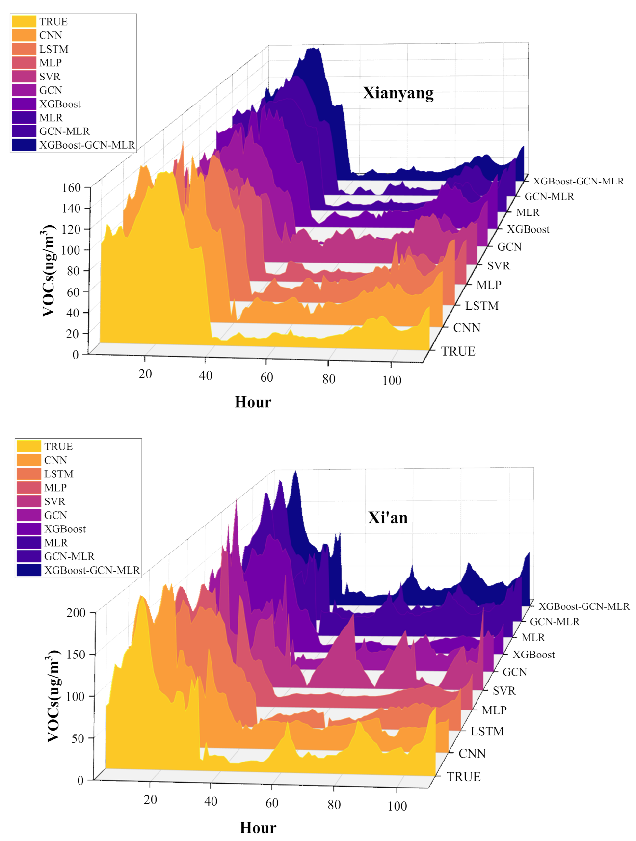
In terms of prediction results, this paper takes the VOCs concentration of the regional grid as the entry point and proposes a concentration prediction-based VOCs aggregation sensing method. It was demonstrated that the combined prediction model proposed in this paper has higher prediction accuracy compared to other deep learning models. In this paper, the prediction results of XGBoost-GCN-MLR are generally better than those of CNN, LSTM, MLP, SVR, GCN, XGBoost, MLR and GCN-MLR, and the results of several experiments show that the proposed model has good robustness.

2. Intelligent Sensing Model of VOCs Gathering Concentrations

2.1. Study Area

The Kuan-chung Plain is located in central Shaanxi Province, between the Qinling Mountains and the northern Weibei Mountains. The Kuan-chung Plain includes Xi’an, Baoji, Xianyang, Weinan and Tongchuan in Shaanxi Province, with a length of about 300 km, an altitude of about 323–800 m and an area of about 49,400 square km. The Kuan-chung Plain has a continental climate with an average annual temperature of 6–13 °C. Annual precipitation ranges from 500 to 800 mm, of which 60% is from June to September, with less precipitation in winter and spring.

2.2. Modelling of VOCs Aggregation in Associated Areas

2.2.1. Regional Gridding

VOCs pollutants in the region will move and accumulate in the near-surface layer of the region due to factors such as meteorological conditions and geographical location. There are different distributions of VOCs concentrations at different locations in the region. In order to implement a fine-grained management of regional VOCs pollutants, the areas are divided into grids. Xi’an, Baoji, Tongchuan, Weinan and Xianyang were selected as the study area. The selected study area was divided into a 10 × 10 km square element grid using the grid division method. The n grids obtained by gridding are numbered 1, 2, …, n, starting from the bottom left corner of the grid range layer. Each grid represents a sub-region and records information on the VOCs data for that sub-region. At the same time, in order to accurately position the regional grid, a coordinate system is established using geographic coordinates as spatial reference information. The centre point of each grid has its own latitude and longitude coordinates. ($x_i$, $y_i$) denotes the coordinates of the centroid of the i-th grid, where i = 1, 2, …, n. In the process of regional grid-based management of VOCs, the number of monitoring points set up in the grid is much smaller than the total number of grids due to financial and geographical constraints. Let there be a monitoring point at grid $i$ in the regional grid map with a monitoring value of $Z_i$. The points not monitored at grid P are called points to be interpolated and their values to be interpolated are denoted by $Z_p$. In order to predict the trend of regional VOCs concentrations and to perceive in time and space the dynamics of VOCs occurring in the region, the inverse distance weighted method was used [41].

$$Z_p={\displaystyle \sum _{i=1}^n\frac{Z_i}{d_i^2}}/{\displaystyle \sum _{i=1}^n\frac{1}{d_i^2}}$$

(1)

where $d_i^{}$ is the distance between the grid to be interpolated and the $i$-th grid in its neighbourhood, $n$ is the number of grids to be divided.

2.2.2. VOCs Aggregation Sensing Model Construction

VOCs aggregation perception is the prediction of VOCs aggregation from the perspective of VOCs aggregation risk and VOCs eventual formation of haze from the perspective of spatial and temporal characteristics. VOCs aggregation sensing is the perception of the direction and state of change of VOCs concentrations as a reflection of their future occurrence in air pollution conditions. In order to reflect the extent of VOCs aggregation in different grids within the correlation area, predictions of VOCs concentrations in the relevant regional grids are required. In this paper, we propose a model for sensing the aggregation of VOCs based on concentration prediction. The model is divided into three parts: XGBoost feature selection, GCN-MLR concentration prediction and VOCs aggregation trend sensing. Taking grid k as an example, a variety of relevant features affecting the variation in VOCs aggregation concentration are first selected, and the known VOCs feature data series are input into the XGBoost feature selection model for feature importance ranking and selection. The new feature data series are obtained by selecting the features that have a greater impact on the variation in VOCs concentrations through the XGBoost model. Using this new feature data series as input to the GCN prediction model, the predicted hourly concentrations of VOCs at time t in the future are obtained by MLR model prediction. The predicted hourly concentrations of VOCs for all grids at time t in the future can be obtained in the same way. Based on the predicted results, the indicators of VOCs aggregation potential for each grid at time t are obtained: T is aggregation time, Weight is the aggregation level weighting. The aggregation time and the aggregation level of VOCs in different grids at the same time are different, so the maximum aggregation time $T_t$ and the maximum aggregation level weight ${\mathit{Weight}}_t$ at time t are selected from the m grids. The number of grids in the region as a whole that exceed the concentration limit at time t is used to represent the range of VOCs aggregation, then the VOCs aggregation potential value $A_t$ for the region as a whole at time t is obtained. Finally, the VOCs aggregation potential perception results are visualised.

2.3. Perceived Extent of VOCs Aggregation

The risk of VOCs aggregation is defined as the severity of the deviation of VOCs concentration values from normal thresholds, expressed as an aggregation level. The degree of aggregation class is defined with reference to the correlation between changes in VOCs and PM_2.5 concentrations during a single episode of heavy pollution [42]. As shown in

Table 1. VOCs aggregation degree.

Number	Concentration	Aggregation	Weights
1	(0, 75)	Good	0
2	(75, 125)	Mild	0.2
3	(125, 160)	Moderate	0.4
4	(160, 190)	Heavy	0.6
5	(190, 260)	Severe	0.8
6	(260, 500)	Extreme	1

, the aggregation levels are defined as follows: Level 1 for non-VOCs pollution, Level 2 for light VOCs pollution, Level 3 for moderate VOCs pollution, Level 4 for moderate to heavy VOCs pollution, Level 5 for heavy VOCs pollution and Level 6 for severe VOCs pollution. The corresponding rank weights are defined as the degree of aggregation: 0 for no aggregation, 0.2 for low aggregation, 0.4 for medium aggregation, 0.6 for medium to high aggregation, 0.8 for high aggregation and 1 for very high aggregation.

The calculation of individual grids and the overall regional VOCs aggregation dynamics considers mainly the threat of haze formation. The higher the VOCs concentration value, the greater the degree of aggregation and the greater the likelihood of haze formation. T represents the time of aggregation of VOCs. As VOCs gradually accumulates VOCs will gradually form a haze. The time at which aggregation occurs in a given grid is calculated cumulatively from the time the concentration value exceeds 75 μg/m³, defaulting the value of T to 1. When the predicted VOCs concentration value for a grid exceeds the threshold and the concentration value for that grid at the next moment is greater than or equal to the concentration value at the previous moment, then T + 1, otherwise T − 1, until T is 0 representing the end of the aggregation time. The aggregation potential value $A_i^t$ of grid i at moment t is then calculated as shown in Equation (2).

$$A_i^t={\mathit{Weight}}_t^k{T}_t^k$$

(2)

where ${\mathit{Weight}}_t^k$ is the aggregation level weight of grid i at time t. $T_t^k$ is the aggregation time of the grid k at moment t. When $A_i^t$ is 0, the grid has a low risk of aggregation or no aggregation. When $A_i^t$ is greater than 0 it indicates that VOCS aggregation is occurring on this grid. A higher value of A indicates a more severe and prolonged accumulation of VOCs in that grid.

Here, the aggregation potential values are calculated for the city as a whole. For the calculation of the overall city VOCs aggregation trend at time t, the trend indicator for the city as a whole is generated from the aggregation trend indicators of individual grids. ${\mathit{Weight}}_t$ is the VOCs aggregation degree level weight, $T_t$ is the time at which aggregation of VOCs occurs, $R_t$ is the extent of VOCs aggregation. The total number of grids into which the study area is divided is indicated by $m$. The extent of VOCs aggregation $R_t$ is expressed as the number of grids in the grid area where the mass concentration of VOCs exceeds 75 μg/m³ and the number of grids with an aggregation level rating of mild and above at time t. Aggregation level weights and aggregation times are taken as maximum values for all grids at the same time. The worst result was selected for the VOCs aggregation level calculation, which was used to indicate the most severe level of aggregation that may exist in the region as a whole. Then, the aggregation potential value for the region as a whole at moment t is calculated as shown in Equation (3).

$$A_t={\mathit{Weight}}_t{T}_t+\frac{R_t}{m}$$

(3)

The degree of aggregation and haze generation can be seen through the aggregation potential value $A_t$. The higher the level of aggregation occurring in the region as a whole, the greater the likelihood of haze formation. If the threat occurs more frequently or for longer periods of time, the more severe the impact on the region as a whole is likely to be. If the VOCs accumulate over a wider area, the wider the range of possible haze formation, where an $A_t$ of 0 indicates a low or no aggregation risk for all grids in the region as a whole. When $A_t$ is not 0, it means that the region as a whole contains grids where aggregation occurs. The value to the right of the decimal point of $A_t$ indicates the ratio of the number of grids exceeding the concentration limit to the total number of grids. The magnitude of the ratio indicates the size of the area where VOCs are concentrated in relation to the total area of the area. When $A_t$ is an integer and not 0, it indicates that VOCs are concentrated over the whole area.

2.4. Data Collection and Pre-Processing

2.4.1. Introduction to the Data

The experimental data used in this paper include VOCs concentration data, air quality data and meteorological data for the period 1 September 2020–31 December 2020. Data were obtained via China Meteorological Administration, China National Environmental Monitoring Centre. The data of the unknown grid was derived from the dataset generated through collation, calculation and spatial interpolation processing with a spatial resolution of 10 × 10 km. In this paper, Xi’an, Baoji, Tongchuan, Weinan and Xianyang were selected as the study area, and the study area was divided into fine grids covering the entire regional geographical area by means of a 10 × 10 km grid division. The grid map is shown in Figure 1.

2.4.2. Data Collection

The existing monitoring equipment not only monitors the concentration of VOCs (emissions per unit volume), but also analyses the content of the different components of VOCs in the area and uploads the monitoring data to a server for storage. For grids with monitoring points, VOCs monitoring values are obtained through monitoring equipment and processed in a uniform format. Monitoring data from known monitoring points were used to calculate the predicted composition of VOCs for grids without monitoring points by inverse distance weighted. The grid monitoring data was combined with the grid prediction data to obtain the VOCs pollutant concentration values for the regional grid, as shown in

Table 2. VOCs emission values of the regional grid.

Pollutants	Grid
	Grid 1	Grid 2	…	Grid n
Benzene	V1(1)	V2(1)	…	Vn(1)
Methylbenzene	V1(2)	V2(2)	…	Vn(2)
⋮	⋮	⋮	⋱	⋮
Styrene	V1(12)	V2(12)	…	Vn(12)

.

The main components of VOCs are numbered sequentially in Table 2: benzene as No. 1, methylbenzene as No. 2, …… and styrene as No. 12. Pollutants are combined with cell grid sequence codes to describe the monitored concentration values of different components in different grids, V₁₍₁₎ for benzene in grid 1, V_n(12) for styrene in grid n, and in turn collected to obtain the concentration values of VOCs pollutants in the regional grid.

2.4.3. VOCs Data Characteristics

As precursors, VOCs react with atmospheric pollutants to form photochemical pollutants such as O₃ and secondary organic matter aerosols (SOA) in response to meteorological factors. Changes in meteorological factors can affect changes in the concentration of VOCs and accompany changes in other pollutants in the atmosphere. Aggregation of regional VOCs occurs and can be influenced by a variety of surrounding environmental factors. Therefore, six major pollutants affecting air quality were selected with 13 collated and more complete meteorological factor statistics as the relevant characteristic variables for VOCs concentration prediction, as shown in

Table 3. Air pollutant and meteorological factors of VOCs aggregation sensing model.

Category	Factors	Representation	Unit
Atmospheric pollutant factors	VOCs	X1	μg/m3
	PM2.5	X2	μg/m3
	PM10	X3	μg/m3
	SO2	X4	μg/m3
	NO2	X5	μg/m3
	O3	X6	μg/m3
	CO	X7	μg/m3
Meteorological factors	Daily average surface temperature	X8	0.1 ℃
	Daily maximum surface temperature	X9	0.1 ℃
	Daily minimum surface temperature	X10	0.1 ℃
	Average wind speed	X11	km/h
	Maximum wind speed	X12	km/h
	Daily maximum wind speed wind direction	X13	-
	Extreme wind speed	X14	km/h
	Average temperature	X15	0.1 ℃
	Highest temperature	X16	0.1 ℃
	Lowest temperature	X17	0.1 ℃
	Hours of sunshine	X18	0.1 h
	Average humidity	X19	1%
	Lowest humidity	X20	1%
	Average air pressure	X21	0.1 hpa
	Lowest air pressure	X22	0.1 hpa

. For grid k, a total of N hours of data are obtained, such that X_k = (X₁, X₂, ⋯, X_N) denotes the time series dataset of grid k and N is the total number of hours in the dataset. Where X_k(t) includes the hourly values of the eigenvariables at moment t and X_k,_j(t) is the jth eigenvalue of grid k at moment t.

3. Methods

3.1. Graph Convolutional Neural Network (GCN)

Graph convolutional neural network (GCN) is a kind of convolutional neural network which is based on graph data. First proposed by Bruna in 2013, the emergence of graph convolutional neural network provides new ideas for processing non-Euclidean graph data. GCN can be applied to social network analysis, recommendation systems and traffic prediction.

The essential purpose of GCN is to use graph convolution to extract spatial features of non-Euclidean structured graph data [43]. For the graph $G=(V,E,A)$, the input signal $X$ and the output signal $Y$, the processing method $f$ adopted by the graph convolutional neural network is defined as:

$$f(X,A)=Y$$

(4)

where $V$ denotes the number of nodes in the graph, and the input features of the n grids at each time point can be translated into a graph signal as a feature matrix $v={\left\{vi\right\}}_{i=1}^N$. $E$ denotes the set of edges, $A$ is the adjacency matrix of the graph, $A\in R^{N\times N}$. The elements in matrix $A$ represent the spatial connectivity between nodes $v_i$ and $v_j$ in graph $G$. The forward propagation formula for the convolution of a graph is:

$$H^{(l+1)}=\sigma ({\tilde{D}}^{-\frac{1}{2}}{\tilde{A}\tilde{D}}^{-\frac{1}{2}}{H}^{(l)}{W}^{(l)})$$

(5)

where, $\tilde{A}=A+I$, I is a unit matrix of size $N\times N$; $\tilde{D}$ is the diagonal matrix, ${\tilde{D}}_{ii}={{\displaystyle \sum }}_j{\tilde{A}}_{ij}$; $H^l\in R^{N\times D}$ denotes the output value of the $l$th level, where $H^0=X$; $\sigma (.)$ denotes the activation function; $w^l$ denotes the parameter value of the $l$th layer.

3.2. Multiple Linear Regression

MLR is a traditional prediction method. The training process has a significant speed advantage over back propagation neural networks and support vector regression (SVR) algorithms. For highly periodic curves, multiple linear regression makes it easier to obtain accurate predictions than neural networks and SVR. The effect is similar to that of a neural network using a linear function as the activation function, but without the tedious iterative training process and parameter tuning. Therefore, for low frequency load components, the use of multiple linear regression is a more suitable option compared to other methods. The strength of the model fit can be diagnosed by judging the normality and independence of the residuals, while the selection of independent variables in the model is often completed using stepwise regression and full subset regression [44].

MLR is a traditional mathematical statistical model with matrix expressions and their expansions as:

$$Y=X\times \beta +\mu$$

(6)

$$\left[\begin{array}{c}{y}_1\\ y_2\\ ⋮\\ y_n\end{array}\right]=\left[\begin{array}{cccc}1& x_{11}& \dots & x_{1n}\\ 1& x_{21}& \dots & x_{2n}\\ ⋮& ⋮& \ddots & ⋮\\ 1& x_{n1}& \dots & x_{\mathit{nn}}\end{array}\right]\times \left[\begin{array}{c}{\beta }_0\\ {\beta }_1\\ {\beta }_2\\ {\beta }_n\end{array}\right]+\left[\begin{array}{c}{\mu }_1\\ {\mu }_2\\ {\mu }_3\\ {\mu }_n\end{array}\right]$$

(7)

$y_i$ indicates the concentration of VOCs; $x_{ij}$ indicates the factors affecting VOCs; ${\beta }_0\left(i=1, 2, \dots , n\right)$ denotes regression coefficient; ${\mu }_i$ denotes random perturbation.

3.3. XGBoost Algorithm

The XGBoost algorithm is a scalable system of tree boosting algorithms based on the idea of integration and is an integration of many categorical regression trees [45]. XGBoost has been widely used in Kaggle competitions, finance and many other fields. This algorithm prevents overfitting of the model by introducing regular terms in the loss function and other methods and can process large amounts of data faster and more efficiently. The most basic predictive model can be expressed as Equation (8):

$${\widehat{y}}_i={\displaystyle \sum _{k=1}^K}{f}_k(x_i),f_k\in F$$

(8)

where, $i$ =1,2,… , $n$, $n$ is the number of samples, $K$ is the number of trees, and $f_k$ is a function in the set $F$ of trees.

The loss function consists of an error term $L(\theta )$ and a regularisation term $\mathsf{\Omega }(\theta )$. The error and regularisation terms are denoted, respectively, as shown in Equation (9) and Equation (10):

$$L(\theta )=l(y_i,{\widehat{y}}_i)={\displaystyle \sum _{i=1}^n}{(y_i-{\widehat{y}}_i)}^2$$

(9)

$$\mathsf{\Omega }(\theta )={\displaystyle \sum _{K=1}^K\mathsf{\Omega }(f_k)}$$

(10)

where $l(y_i,{\widehat{y}}_i)$ is the training error of ix of the sample and $\mathsf{\Omega }(f_k)$ is the regular term of the $k$-th tree.

A further Taylor expansion of the loss function yields an approximate objective function as shown in Equation (11):

$$\begin{array}{l}L(\varphi )\cong {\displaystyle \sum _{i=1}^n[l(y_i,{{\widehat{y}}_i}^{\left(t-1\right)})g_i{f}_t(x_i)+\frac{1}{2}{h}_i{f}_t^2(x_i)]}+\mathsf{\Omega }(\theta )+C\\ g_i=f_i^{\text{'}}(x_i), h_i=f_i^{″}(x_i)\end{array}$$

(11)

where $f_t(x_i)$ denotes the new function added for the $t$-th time and $C$ is a constant term. Here, let $G_j={\displaystyle \sum _{i\in I_j}{g}_i}$, $H_j={\displaystyle \sum _{i\in I_j}{h}_i+\lambda }$, then we get Equation (12):

$${\omega }_j*=-\frac{-G_j}{H_j+\lambda }$$

(12)

Using the greedy algorithm, a new segmentation is added each time to an existing leaf and the maximum gain obtained as a result. For a specific segmentation scheme, the gain obtainable is calculated as in Equation (13).

$$\mathit{Gain}=\frac{1}{2}[\frac{G_L^2}{H_L^2+\lambda }+\frac{G_R^2}{H_R^2+\lambda }+\frac{{(G_L+G_R)}^2}{H_R^2{H}_L^2+\lambda }]-\gamma$$

(13)

where term 1 represents the gain resulting from splitting the left subtree, term 2 represents the gain resulting from splitting the right subtree, term 3 represents the gain without splitting and $\gamma$ represents the complexity cost due to the addition of new leaves to the split.

3.4. Intelligent Sensing Model for VOCs Aggregation

Based on historical data and area gridding, we propose a hybrid model to predict future VOCs concentrations at different time spans at hourly scales. The schematic diagram of our proposed model based on the XGBoost-GCN-MLR structure is shown in Figure 2. The correlation region is first divided into a grid, and then the features are ranked by importance using XGBoost. Further, the feature-selected data is fed into the GCN and spatial features are extracted using graph convolution operations. Extraction of temporal features of VOCs is completed using MLR. In our framework, the input to MLR is a graph convolution feature connected to the original signal. Within each spatio-temporal block, the graph signal and spatial weight matrix are extracted for each time point and the spatial features are calculated by graph convolution. The graphic signal is then connected to the MLR. Finally, the output of the MLR was used as a prediction of the expected time VOCs concentration.

3.5. Evaluation Indicators

In order to verify the performance of the model, the error indicator in this paper uses Root Mean Square Error (RMSE), Mean Absolute Error (MAE), Mean Absolute Percentage Error (MAPE) and R² as evaluation indicators [46].

$$\mathrm{RMSE}=\sqrt{\frac{1}{N}{\displaystyle \sum _{i=1}^N{({\widehat{y}}_i-y_i)}^2}}$$

(14)

$$\mathrm{MAE}=\frac{1}{N}{\displaystyle \sum _{i=1}^N|{\widehat{y}}_i-y_i{|}^2}$$

(15)

$$\mathrm{MAPE}=\frac{100}{N}{\displaystyle \sum _{i=1}^N}|\frac{{\widehat{y}}_i-y_i}{y_i}|$$

(16)

$$R^2=1-\frac{{\displaystyle \sum _i}{({\widehat{y}}_i-y_i)}^2}{{\displaystyle \sum _i{(\overline{y}-y_i)}^2}}$$

(17)

where, ${\widehat{y}}_i$ represents the predicted VOCs mass concentration at point $i$; $y_i$ represents the actual VOCs mass concentration at point $i$; $\overline{y}$ is the mean of the modelled VOCs mass concentration in the corresponding dataset; $N$ is the number of samples in the dataset [47].

4. Results

4.1. Feature Selection

XGBoost obtains the importance of each feature from the tree after gradient boosting. The importance of a feature indicates the role of this feature in the construction of the lifting tree [48]. A feature is more important if it is used as a dividing attribute more often in all trees. The importance of individual decision trees is calculated by the amount of each attribute partition point improvement performance measure, weighted by the number of observations for which the node is responsible. Finally, the element importance is averaged across all decision trees in the model. The final importance of each feature is obtained, after which the features can be ranked or compared with each other.

In VOCs concentration prediction, feature selection can reduce the complexity of the prediction model and improve the prediction accuracy. Therefore, the XGBoost model was used to rank the feature variables involved in VOCs concentration prediction in terms of feature importance and select the variables that have a greater impact on VOCs concentration prediction. The step size indicates the length of the historical time series data on which each prediction relies. The importance analysis of VOCs-related feature variables was carried out based on XGBoost using Grid 92 as an example. After several experiments, it was found that the model prediction error was minimised by selecting the top 10 feature variables among the feature variables with a step size of 3 for each input as the input feature variables for the GCN-MLR model.

We used the training set part for feature filtering to divide the dataset into a training set and a validation set. For different classification problems, feature selection can effectively remove the redundant elements in the feature set, which can have the effect of improving the generalisation performance of the model. Firstly, the importance ranking of all features is obtained based on XGBoost. The top-ranked features are then added to the feature subset (initially the empty set) in turn, and the cross-checked classification accuracy (ACC) of the feature subset is calculated after each addition. If the ACC improves, the feature is retained, and if not, the feature is removed, and the optimal feature subset is obtained by iterating through all features. Cross-validation is used for the training and validation sets to select the optimal hyperparameters, and the training and validation sets are trained together to produce the final model. GBtree was chosen as the weak evaluator for this model. Detailed parameters are set as follows: Num-class was set to 4, n-estimators was set to 130, the learning rate was set to 0.3 by default, and max-depth was set to 6 for the best accuracy of the model.

The different features of the five cities are ranked in importance by the XGBoost algorithm. The top 10 feature importance values for the five cities are shown in Figure 3, with the y-axis representing the cities and the x-axis representing the features. The colour shades of the squares represent the magnitude of feature importance. The importance of the features differs for different regional VOCs and the filtered features are fed into GCN-MLR

4.2. VOCs Concentration Prediction Based on XGBoost-GCN-MLR Model

As shown in Figure 4, a comparison of the five cities shows that the XGBoost prediction model and the GCN prediction model are more inaccurate in predicting VOCs concentrations at the spikes. The MLR model is less effective in predicting VOCs concentrations at the lower true values. CNN, LSTM and MLP are less effective in prediction when the VOCs concentration values fluctuate widely. The overall predicted value of SVR is greater than the actual value. The XGBoost-GCN-MLR prediction model in Figure 4 is more accurate in predicting VOCs at the spikes, thus indicating that the GCN-MLR prediction model with feature extraction is more accurate in predicting sudden changes in VOCs concentrations. As can be seen from Figure 4, the predicted hourly VOCs concentrations of the XGBoost-GCN-MLR model are close to the measured values, and when the measured hourly VOCs concentrations increase rapidly, the predicted values deviate little from the measured values. The four models, CNN, LSTM, MLP and SVR, showed large deviations between the predicted and measured values when the measured values increased or decreased sharply. When the measured values of the GCN-MLR model were between 40 and 80 ug/m³, the predicted and measured hourly concentrations of VOCs were more consistent, and when the measured values were greater than 100 μg/m³, the predicted values were greater than the measured values. The GCN model predicted values were significantly smaller than the measured values. Comparing the predicted hourly VOCs concentrations of the nine models with the measured values in five cities, the XGBoost-GCN-MLR model predicted the best results.

As can be seen from

Table 4. Accuracy comparison of nine models in five cities.

City	Evaluation Index	CNN	LSTM	MLP	SVR	GCN	XGBoost	MLR	GCN-MLR	XGBoost- GCN-MLR
Baoji	RMSE	8.7331	8.9924	8.8620	13.0087	8.377	5.252	5.9861	4.4833	3.2436
	MAE	6.2389	6.4813	6.0716	10.3413	6.0049	4.2827	3.9951	3.4183	2.9516
	MAPE	0.2610	0.3291	0.2122	0.8211	0.2201	0.2932	0.1025	0.1364	0.0685
	R2	0.7943	0.7879	0.7912	0.7655	0.8028	0.8618	0.8503	0.8721	0.8979
Tongchuan	RMSE	17.0812	11.7999	12.0799	13.0087	11.6993	10.0232	9.7749	6.5573	5.4892
	MAE	11.2308	9.6179	9.1894	10.3413	8.4598	8.8154	6.2045	4.6676	4.1168
	MAPE	0.2100	0.2209	0.2013	0.8211	0.204	0.4016	0.1555	0.1305	0.1019
	R2	0.7719	0.8389	0.8359	0.7955	0.8399	0.8559	0.858	0.8811	0.8947
Weinan	RMSE	12.7652	22.3230	12.2303	17.8997	10.2787	12.2824	7.0161	6.3676	5.2561
	MAE	8.4136	16.1408	7.8273	13.3125	6.7729	10.1576	5.9529	4.3599	3.9111
	MAPE	0.2811	0.3963	0.1810	0.7880	0.1789	0.4881	0.3732	0.1276	0.1192
	R2	0.8520	0.7532	0.8559	0.8056	0.8689	0.8556	0.8855	0.8881	0.8985
Xi’an	RMSE	26.8876	23.4873	23.9599	33.0032	11.6993	10.1385	10.0232	6.5573	3.4892
	MAE	19.6508	17.7037	17.9471	26.3624	8.4598	8.2763	8.8154	4.6676	3.1168
	MAPE	0.4780	0.4046	0.5651	0.7818	0.2040	0.1688	0.4016	0.1019	0.1305
	R2	0.6825	0.7577	0.7479	0.5217	0.8399	0.8511	0.8559	0.8811	0.8947
Xianyang	RMSE	21.997	20.085	22.9112	29.9232	19.6825	15.6156	10.7567	9.0542	6.6113
	MAE	16.301	15.617	12.2295	23.971	12.476	11.974	5.6525	5.8845	4.3458
	MAPE	0.6324	0.6369	0.2118	1.0896	0.348	0.4199	0.0897	0.1984	0.063
	R2	0.7311	0.7592	0.8168	0.6875	0.8648	0.8149	0.8596	0.8714	0.8991

, compared with the CNN prediction model, the RMSE, MAE and MAPE of the XGBoost-GCN-MLR prediction model were reduced by an average of 69.3%, 65.41% and 69.11%, respectively, in the five cities. Compared with the LSTM prediction model, the RMSE, MAE and MAPE of the XGBoost-GCN-MLR prediction model were reduced by an average of 69.22%, 68.4% and 72.17%, respectively, in the five cities. Compared with the SVR prediction model, the RMSE, MAE and MAPE of the XGBoost-GCN-MLR prediction model were reduced by an average of 66.31%, 60.74% and 59.68%, respectively, in the five cities. Compared to the GCN prediction model, the RMSE, MAE, MAPE and SMAPE of the XGBoost-GCN-MLR prediction model were reduced by an average of 59.96%, 54.55%, 58.55% and 56.54%, respectively, in the five cities. Compared with the XGBoost prediction model, the RMSE, MAE, MAPE and SMAPE of the XGBoost-GCN-MLR prediction model were reduced by 52.79%, 54.38%, 77.96% and 66.51% on average in the five cities, respectively. In contrast to the MLR prediction model, the RMSE, MAE, MAPE and SMAPE of the XGBoost-GCN-MLR prediction model were reduced by an average of 43.69%, 36.37%, 41.37% and 45.12%, respectively, in the five cities. Compared to the GCN-MLR prediction model, the RMSE, MAE, MAPE and SMAPE of the XGBoost-GCN-MLR prediction model were reduced by an average of 27.03%, 19.02%, 36.63% and 30.69%, respectively, in the five cities. Compared with the other four models, the XGBoost-GCN-MLR-based VOCs concentration prediction model improved in terms of prediction accuracy. By calculating the R², RMSE, MAE and MAPE of the measured and predicted values, the R² of the nine machine learning models ranged from 0.6825 to 0.8991, and the results were quite satisfactory. Among them, the XGBoost-GCN-MLR model and the GCN-MLR model both have R² greater than 0.87, while the rest of the models have values below 0.87. The RMSE of the models ranged from 11.13 to 26.88 in the five cities. The XGBoost-GCN-MLR model has the lowest RMSE value in all five cities, while the CNN model has the highest RMSE value of 26.88 in Xi’an. Comparing the MAE values, the XGBoost-GCN-MLR model has the lowest MAE value of 2.9516 in Baoji, followed by the GCN-MLR model with 3.4183 and the maximum MAE value of 19.6508 for the CNN model. For the MAPE metric, the XGBoost-GCN-MLR model also had the lowest value of the nine models, with an average of 0.09662 across the five cities. The average MAPE of the remaining models was greater than 0.13 in all five cities, while the MAPE of the CNN and LSTM models was greater than 0.3. When comparing the nine machine learning models, the XGBoost-GCN-MLR model has the best prediction performance followed by the GCN-MLR model, while the CNN and LSTM models have poor prediction ability among the nine models.

The XGBoost-GCN-MLR prediction model outperforms the GCN, XGBoost and MLR prediction models, and the predicted values fit the true value curve better. The GCN-MLR model using the GCN algorithm gives better predictions than the single deep learning model MLR model, which in turn is more suitable than the three models CNN, MLP and SVR for the prediction of VOCs mass concentration data in this paper. The XGBoost-GCN-MLR prediction model uses the XGBoost model to select the feature variables in a meritocratic manner, optimising the number of model input feature variables and reducing the complexity of model construction. The proposed model fully exploits the relationship between time series data and learns the long-term dependence in historical time series data, achieving better prediction results.

4.3. DM Test

The main objective of the DM test is to test whether there is a significant difference in the predictive power between the baseline model and the model under test. The original hypothesis H0 of the DM test is that the baseline model outperforms the prediction accuracy of the tested model. The alternative hypothesis H1 of the DM test is that the prediction accuracy of the tested model outperforms the prediction accuracy of the baseline model. The DM tests are shown in

Table 5. DM test.

Compared Algorithm	DM	P(DM)
CNN	−7.3356	1.6635 × 10−6
LSTM	−8.4718	2.4563 × 10−5
MLP	−7.3629	2.1878 × 10−5
SVR	−7.5231	3.7718 × 10−4
GCN	−6.6567	5.3325 × 10−4
XGBoost	−6.6209	2.354 × 10−4
MLR	−3.7377	3.265 × 10−4
GCN-MLR	−3.6826	2.5689 × 10−3

. Since the p-values of all eight prediction models are less than 0.05, the results of the DM test indicate that the XGBoost-GCN-MLR method proposed in this paper can make accurate predictions of directional changes in the original data when compared to all eight models. The horizontal prediction ability of the XGBoost-GCN-MLR method was significantly better than the prediction ability of the remaining eight comparison models, and the DM test results show that XGBoost-GCN-MLR can effectively improve the prediction accuracy of the hourly VOCs concentrations.

From Table 5, the DM test results show that the predictive power of the other eight algorithms is significantly different compared to the XGBoost-GCN-MLR model. The associated p-value for each DM statistic was less than α at the α = 0.05 level. Confidence and significance results indicated that the XGBoost-GCN-MLR model had better predictive power than similar algorithms.

4.4. Robustness Test

The stability of a predictive model has an important impact on the scope of its application. Models with high stability are better able to withstand external disturbances and ensure the reliability of prediction results. To assess the robustness of the model to outliers, the test dataset was retested after perturbation. Random Gaussian noise of 5% and 10% was added to the model input parameters. The XGBoost-ETPGMLP maintained good prediction results under 5% noise perturbation. As shown in

Table 6. Comparison of mean absolute error of VOCs in Xi’an.

Data	Error Values/(ug/m3)
	CNN	LSTM	MLP	SVR	GCN	XGBoost	MLR	GCN- MLR	XGBoost- GCN-MLR
Normal	19.6508	17.7037	17.9471	26.3624	8.4598	8.2763	8.8154	4.6676	3.1168
5%Noise	22.5002 (+14.5%)	20.4832 (+15.7%)	20.5674 (+14.6%)	30.0795 (+14.1%)	9.6188 (+13.7%)	9.3274 (+12.7%)	9.8115 (+11.3%)	5.0550 (+8.3%)	3.2321 (+3.7%)
10%Noise	28.3727 (+26.1%)	25.6654 (+25.3%)	25.6270 (+24.6%)	37.0579 (+23.2%)	11.5618 (+20.2%)	11.3421 (+21.6%)	11.6561 (+18.8%)	5.9093 (+16.9%)	3.5036 (+8.4%)

, compared with the other eight models, the XGBoost-GCN-MLR error increased by only 3.7%, while the error increased by 8.4% under 10% noise perturbation.

4.5. VOCs Aggregation Perception Analysis

Based on the predicted VOCs concentration results, the aggregation potential value $A_i^t$ of each grid is calculated by Equation (2). The magnitude of the aggregation potential value of each grid is represented by different shades of colour, the darker the colour the larger the aggregation potential value, the lightest colour grid has an aggregation potential value of 0. The overall VOCs aggregation trend in the region is shown in Figure 5. The distribution of the VOCs aggregation pattern for each grid in the study area at 14:00 (t = 134) on 8 December 2020 was obtained by ArcGIS as shown in Figure 6. The ratio of the number of grids exceeding the concentration limit to the total number of grids is calculated by using Equation (3) to calculate the VOCs aggregation potential of the region as a whole. The results of the $A_t$ part of Xi’an are shown in

Table 7. Aggregate situation values.

t	Weight	T	At	t	Weight	T	At	t	Weight	T	At
1	0	0	0	50	0.2	1	0.21532	102	0.4	18	7.4
2	0.2	1	0.21532	54	0.2	1	0.21532	106	0.4	18	7.4
6	0.2	1	0.34132	58	0.2	3	0.64596	110	0.4	14	5.8
10	0	0	0	62	0.2	2	0.46128	114	0.6	18	11
14	0	0	0	66	0	0	0	118	0.6	18	11
18	0	0	0	70	0	0	0	122	0.6	20	12.2
22	0.2	2	0.41532	74	0.2	4	0.92256	126	0.6	20	12.2
26	0.2	2	0.43064	78	0.2	3	0.72256	130	0.4	18	7.4
30	0.2	1	0.23064	82	0.2	6	1.29192	134	0.4	15	6.1686
34	0.2	4	0.83064	86	0.2	4	0.96852	138	0	0	0
38	0.2	1	0.21532	90	0.2	8	1.78382	142	1	1	0.2766
42	0	0	0	94	0.2	12	2.6	146	1	2	0.44596
46	0	0	0	98	0.4	16	6.6	150	1	2	0.41532

. Figure 5 shows that the concentration of VOCs in the region as a whole is low and the risk of aggregation is low or non-existent, and no VOCs aggregation warning is required. From Figure 5 and Table 7, it can be seen that at the 94th hour (22:00 on 6 December 2020), the VOCs concentration started to increase significantly and the trend value was 2.6. Indicating that the overall regional VOCs concentration continued to increase and the VOCs aggregation occurred.

From Figure 5, Figure 6 and Table 7, it can be seen that at hour 134 (14:00 on 8 December 2020), on the regional grid VOCs aggregation potential distribution map, the grid with the largest aggregation potential dropped to 6.1686 at this time. This indicates that a grid of VOCs still exists in the region as a whole with 87.41% of the total area of the region where VOCs accumulation occurs, which is consistent with the haze generation in the study area during this time period. The results of the calculations are visualised in Figure 5 and Figure 6 to provide a visual understanding of the distribution of VOCs at a resolution of 10 × 10 km in terms of aggregation dynamics and the direction of the overall regional aggregation dynamics.

5. Conclusions

This paper presented a method for situational awareness of VOCs aggregation based on VOCs concentration prediction. In order to improve the construction efficiency and prediction accuracy of the prediction model, the XGBoost model was used to select the importance of VOCs-related features. A VOCs concentration prediction model based on XGBoost-GCN-MLR was constructed, and VOCs aggregation trend indicators were generated for VOCs aggregation trend perception analysis. The results showed that the proposed XGBoost-GCN-MLR-based VOCs prediction model handled the VOCs concentration time series with higher prediction accuracy than other models, and the RMSE, MAE and MAPE were reduced by 57.81%, 54.17% and 62.98%, respectively. VOCs aggregation situational awareness provides managers with a concise and intuitive view of VOCs aggregation in the form of a regional grid situational distribution and an overall regional situational trend map. Finally, by combining the regional grid number and coordinate information, we can precisely locate the areas where the future VOCs aggregation is in a more serious situation. The proposed model can provide decision support to managers for early warning information expression, which is important for VOCs management and environmental protection.

The recommendations made in this paper are as follows:

(1)

Grid-based management of associated regions for joint prevention and control. Grid management is a key step in the refinement of regional management and the basis for pollution prevention and control. Information from different grids can be shared, and pollution from each grid can be monitored and summarised in real time.

(2)

Use the degree of influence of VOCs pollution between associated areas to apply preventive and control measures to the relevant areas. Monitor the pollution concentration in each sub-regional grid and propose relevant guidelines to reduce pollution and harm to the environment according to local conditions. VOCs emissions from different grid areas will be aggregated, with key monitoring of heavily polluted areas and timely release of grid and source information for heavily polluted areas. VOCs are also controlled at the source, regulated in the process and treated at the end of the process.

(3)

Prediction and early warning of VOCs pollution. The sources of VOCs pollution are identified through immediate prediction and early warning to further strengthen the management of pollution control. At the same time, the functions and tasks of each organisation’s personnel are assigned according to the degree of VOCs aggregation in the grid, and the relevant personnel are involved in timely follow-up and feedback.

References

1. Sun, Y.; Jiang, Q.; Wang, Z.; Fu, P.; Li, J.; Yang, T.; Yin, Y. Investigation of the sources and evolution processes of severe haze pollution in Beijing in January 2013. J. Geophys. Res.-Atmos. 2014, 119, 4380–4398. [Google Scholar] [CrossRef]
2. Jiang, Z.; Grosselin, B.; Daële, V.; Mellouki, A.; Mu, Y. Seasonal and diurnal variations of BTEX compounds in the semi-urban environment of Orleans, France. Sci. Total Environ. 2017, 574, 1659–1664. [Google Scholar] [CrossRef] [PubMed]
3. Delfino, R.J. Epidemiologic evidence for asthma and exposure to air toxics: Linkages between occupational, indoor, and community air pollution research. Environ. Health Perspect. 2002, 110, 573–589. [Google Scholar] [CrossRef] [PubMed]
4. Windham, G.C.; Zhang, L.; Gunier, R.; Croen, L.A.; Grether, J.K. Autism spectrum disorders in relation to distribution of hazardous air pollutants in the San Francisco Bay area. Environ. Health Perspect. 2006, 114, 1438–1444. [Google Scholar] [CrossRef] [Green Version]
5. Zhou, J.; You, Y.; Bai, Z.; Hu, Y.; Zhang, J.; Zhang, N. Health risk assessment of personal inhalation exposure to volatile organic compounds in Tianjin, China. Sci. Total Environ. 2011, 409, 452–459. [Google Scholar] [CrossRef]
6. Tagiyeva, N.; Sheikh, A. Domestic exposure to volatile organic compounds in relation to asthma and allergy in children and adults. Expert Rev. Clin. Immunol. 2014, 10, 1611–1639. [Google Scholar] [CrossRef]
7. Zhou, Y.; Zhang, S.; Li, Z.; Zhu, J.; Bi, Y.; Bai, Y.; Wang, H. Maternal benzene exposure during pregnancy and risk of childhood acute lymphoblastic leukemia: A meta-analysis of epidemiologic studies. PLoS ONE 2014, 9, e110466. [Google Scholar] [CrossRef]
8. Huang, R.J.; Zhang, Y.; Bozzetti, C.; Ho, K.F.; Cao, J.J.; Han, Y.; Prévôt, A.S. High secondary aerosol contribution to particulate pollution during haze events in China. Nature 2014, 514, 218–222. [Google Scholar] [CrossRef] [Green Version]
9. Li, J.; Tang, Z.; Chen, J. Migration Model of VOCs in Composite Package Materials. China Print. Packag. Study 2012, 4, 62–66. [Google Scholar]
10. Zhang, W.; Tan, L.; Wang, Z.; Zhu, W.; Lu, Y.; Li, L. Assessment on VOCs in atmospheric air and their influence to health at Shapingba district of Chongqing city. China Meas. Test 2017, 43, 43–48. [Google Scholar]
11. Zeng, J.; Han, G.; Wu, Q.; Tang, Y. Effects of agricultural alkaline substances on reducing the rainwater acidification: Insight from chemical compositions and calcium isotopes in a karst forests area. Agric. Ecosyst. Environ. 2020, 290, 106782. [Google Scholar] [CrossRef]
12. Zeng, J.; Yue, F.; Li, S.-L.; Wang, Z.; Wu, Q.; Qin, C.; Yan, Z. Determining rainwater chemistry to reveal alkaline rain trend in Southwest China: Evidence from a frequent-rainy karst area with extensive agricultural production. Environ. Pollut. 2020, 266, 115166. [Google Scholar] [CrossRef]
13. Zhang, R.; Wang, H.; Tan, Y.; Zhang, M.; Zhang, X.; Wang, K.; Xiong, J. Using a machine learning approach to predict the emission characteristics of VOCs from furniture. Build. Environ. 2021, 196, 107786. [Google Scholar] [CrossRef]
14. Nkeshita, F.C.; Adekunle, A.A.; Abegunrin, A. Prediction of Indoor Total Volatile Organic Compound in a University Hostel Using a Neural Network Model. NIJOTECH 2021, 40, 186–190. [Google Scholar] [CrossRef]
15. Zhang, Q. Concentration Inversion of Multi-Component Volatile Organic Compounds Based on Deep Neural Network; Xi’an Institute of Optics & Precision Mechanics, Chinese Academy of Sciences: Xi’an, China, 2019. [Google Scholar]
16. Ren, W.; Niu, Y. Application of GA-BP in VOCs Prediction Model in Chemical Industrial Parks. Comput. Appl. Softw. 2018, 35, 274–277. [Google Scholar]
17. Zhao, L. Studies on Respone Interference of VOCs Gas Mixture and Recognition with Neural Network. Master’s Thesis, Dalian University of Technology, Dalian, China, 2017. [Google Scholar]
18. Chen, Z. Research on VOCs Mixed Gas Detection Based on BP Neural Network. Master’s Thesis, Ningbo University, Ningbo, China, 2017. [Google Scholar]
19. Yang, M.; Fan, H.; Zhao, K. PM2.5 prediction with a novel multi-step-ahead forecasting model based on dynamic wind field distance. Int. J. Environ. Res. Public Health 2019, 16, 4482. [Google Scholar] [CrossRef] [Green Version]
20. Ghahremanloo, M.; Choi, Y.; Sayeed, A.; Salman, A.K.; Pan, S.; Amani, M. Estimating daily high-resolution PM2. 5 concentrations over Texas: Machine Learning approach. Atmos. Environ. 2021, 247, 118209. [Google Scholar] [CrossRef]
21. Feng, R.; Gao, H.; Luo, K.; Fan, J.R. Analysis and accurate prediction of ambient PM2. 5 in China using Multi-layer Perceptron. Atmos. Environ. 2020, 232, 117534. [Google Scholar] [CrossRef]
22. Dai, H.; Huang, G.; Wang, J.; Zeng, H.; Zhou, F. Prediction of Air Pollutant Concentration Based on One-Dimensional Multi-Scale CNN-LSTM Considering Spatial-Temporal Characteristics: A Case Study of Xi’an, China. Atmosphere 2021, 12, 1626. [Google Scholar] [CrossRef]
23. Dhakal, S.; Gautam, Y.; Bhattarai, A. Exploring a deep LSTM neural network to forecast daily PM2.5 concentration using meteorological parameters in Kathmandu Valley, Nepal. Air Qual. Atmos. Health 2021, 14, 83–96. [Google Scholar] [CrossRef]
24. Park, Y.; Kwon, B.; Heo, J.; Hu, X.; Liu, Y.; Moon, T. Estimating PM2.5 concentration of the conterminous United States via interpretable convolutional neural networks. Environ. Pollut. 2020, 256, 113395. [Google Scholar] [CrossRef]
25. Lv, B.; Cobourn, W.G.; Bai, Y. Development of nonlinear empirical models to forecast daily PM2.5 and ozone levels in three large Chinese cities. Atmos. Environ. 2016, 147, 209–223. [Google Scholar] [CrossRef]
26. Al-Qaness, M.A.; Fan, H.; Ewees, A.A.; Yousri, D.; Elaziz, M.A. Improved ANFIS model for forecasting Wuhan City air quality and analysis COVID-19 lockdown impacts on air quality. Environ. Res. 2021, 194, 110607. [Google Scholar] [CrossRef]
27. Prihatno, A.T.; Nurcahyanto, H.; Ahmed, M.; Rahman, M.; Alam, M.; Jang, Y.M. Forecasting PM2.5 Concentration Using a Single-Dense Layer BiLSTM Method. Electronics 2021, 10, 1808. [Google Scholar] [CrossRef]
28. Guo, H.; Guo, Y.; Zhang, W.; He, X.; Qu, Z. Research on a Novel Hybrid Decomposition–Ensemble Learning Paradigm Based on VMD and IWOA for PM2.5 Forecasting. Int. J. Environ. Res. Public Health 2021, 18, 1024. [Google Scholar] [CrossRef]
29. Huang, G.; Li, X.; Zhang, B.; Ren, J. PM2.5 concentration forecasting at surface monitoring sites using GRU neural network based on empirical mode decomposition. Sci. Total Environ. 2021, 768, 144516. [Google Scholar] [CrossRef]
30. Photphanloet, C.; Lipikorn, R. PM10 concentration forecast using modified depth-first search and supervised learning neural network. Sci. Total Environ. 2020, 727, 138507. [Google Scholar] [CrossRef]
31. Durao, R.M.; Mendes, M.T.; Pereira, M.J. Forecasting O3 levels in industrial area surroundings up to 24 h in advance, combining classification trees and MLP models. Atmos. Pollut. Res. 2016, 7, 961–970. [Google Scholar] [CrossRef] [Green Version]
32. Liu, T.; Lau, A.K.; Sandbrink, K.; Fung, J.C. Time series forecasting of air quality based on regional numerical modeling in Hong Kong. J. Geophys. Res.-Atmos. 2018, 123, 4175–4196. [Google Scholar] [CrossRef] [Green Version]
33. Zhu, S.; Qiu, X.; Yin, Y.; Fang, M.; Liu, X.; Zhao, X.; Shi, Y. Two-step-hybrid model based on data preprocessing and intelligent optimization algorithms (CS and GWO) for NO2 and SO2 forecasting. Atmos. Pollut. Res. 2019, 10, 1326–1335. [Google Scholar] [CrossRef]
34. Nourani, V.; Karimzadeh, H.; Baghanam, A.H. Forecasting CO pollutant concentration of Tabriz city air using artificial neural network and adaptive neuro-fuzzy inference system and its impact on sustainable development of urban. Environ. Earth Sci. 2021, 80, 136. [Google Scholar] [CrossRef]
35. Wong, P.Y.; Lee, H.Y.; Chen, Y.C.; Zeng, Y.T.; Chern, Y.R.; Chen, N.T.; Wu, C.D. Using a land use regression model with machine learning to estimate ground level PM2.5. Environ. Pollut. 2021, 277, 116846. [Google Scholar] [CrossRef] [PubMed]
36. Just, A.C.; Arfer, K.B.; Rush, J.; Dorman, M.; Shtein, A.; Lyapustin, A.; Kloog, I. Advancing methodologies for applying machine learning and evaluating spatiotemporal models of fine particulate matter (PM2.5) using satellite data over large regions. Atmos. Environ. 2020, 239, 117649. [Google Scholar] [CrossRef] [PubMed]
37. Muthukumar, P.; Cocom, E.; Nagrecha, K.; Comer, D.; Burga, I.; Taub, J.; Pourhomayoun, M. Predicting PM2.5 atmospheric air pollution using deep learning with meteorological data and ground-based observations and remote-sensing satellite big data. Air Qual. Atmos. Health 2021, 11, 1–14. [Google Scholar] [CrossRef]
38. Qi, Y.; Li, Q.; Karimian, H.; Liu, D. A hybrid model for spatiotemporal forecasting of PM2.5 based on graph convolutional neural network and long short-term memory. Sci. Total Environ. 2019, 664, 1–10. [Google Scholar] [CrossRef]
39. Ren, M.; Sun, W.; Chen, S. Combining machine learning models through multiple data division methods for PM2.5 forecasting in Northern Xinjiang, China. Environ. Monit. Assess. 2021, 193, 476. [Google Scholar] [CrossRef]
40. Kim, S.M.; Koo, J.H.; Lee, H.; Mok, J.; Choi, M.; Go, S.; Kim, J. Comparison of PM2.5 in Seoul, Korea Estimated from the Various Ground-Based and Satellite AOD. Appl. Sci. 2021, 11, 10755. [Google Scholar] [CrossRef]
41. Chen, C.C.; Wang, Y.R.; Yeh, H.Y.; Lin, T.H.; Huang, C.S.; Wu, C.F. Estimating monthly PM2.5 concentrations from satellite remote sensing data, meteorological variables, and land use data using ensemble statistical modeling and a random forest approach. Environ. Pollut. 2021, 291, 118159. [Google Scholar] [CrossRef]
42. Lu, X. Characteristics of O3 and PM2.5 Complex Pollution and the VOCs Contributions in Handan. Master’s Thesis, Hebei University of Engineering, Handan, China, 2020. [Google Scholar]
43. Kipf, T.N.; Welling, M. Semi-supervised classification withgraph convolutional networks. arXiv 2016, arXiv:1609.02907. [Google Scholar]
44. You, S.; Yan, Y. Stepwise Regression Analysis and Its Application. Stat. Decis. 2017, 14, 31–35. [Google Scholar]
45. Ribeiro, M.T.; Singh, S.; Guestrin, C. Proceedings of the 22nd ACM SIGKDD International Conference on Knowledge Discovery and Data Mining-KDD’16; Association for Computing Machinery: New York, NY, USA, 2016. [Google Scholar]
46. Kim, T.Y.; Cho, S.B. Predicting residential energy consumption using CNN-LSTM neural networks. Energy 2019, 182, 72–81. [Google Scholar] [CrossRef]
47. Lu, H.; Azimi, M.; Iseley, T. Short-term load forecasting of urban gas using a hybrid model based on improved fruit fly optimization algorithm and support vector machine. Energy Rep. 2019, 5, 666–677. [Google Scholar] [CrossRef]
48. Dai, H.; Huang, G.; Zeng, H.; Yang, F. PM2.5 Concentration Prediction Based on Spatiotemporal Feature Selection Using XGBoost-MSCNN-GA-LSTM. Sustainability 2021, 13, 12071. [Google Scholar] [CrossRef]
Figure 1. Mesh division diagram of Xi’an, Baoji, Tongchuan, Weinan and Xianyang.
Atmosphere 13 00483 g001
Figure 2. VOCs aggregation intelligent sensing model structure.
Atmosphere 13 00483 g002
Figure 3. Characteristic variables with the highest importance of characteristics in the five cities.
Atmosphere 13 00483 g003
Figure 4. Fit curves of predicted and true values of nine models in five cities.
Atmosphere 13 00483 g004aAtmosphere 13 00483 g004b
Figure 5. VOCs trend of the situation value.
Atmosphere 13 00483 g005
Figure 6. Distribution of the VOCs aggregation pattern in the regional grid at 14:00 (t = 134) on 8 December 2020.
Atmosphere 13 00483 g006