Article

Observed Climatology and Trend in Relative Humidity, CAPE, and CIN over India

by
Pathan Imran Khan
1,
Devanaboyina Venkata Ratnam
1,*,
Perumal Prasad
2,
Ghouse Basha
2,
Jonathan H. Jiang
3,
Rehana Shaik
4,
Madineni Venkat Ratnam
2 and
Pangaluru Kishore
5
1
Department of Electronics and Communications Engineering, Koneru Lakshmaiah Education Foundation, Guntur 522502, India
2
National Atmospheric Research Laboratory, Department of Space, Gadanki 517112, India
3
Jet Propulsion Laboratory, California Institute of Technology, Pasadena, CA 91109, USA
4
Hydroclimatic Research Group, Lab for Spatial Informatics, International Institute of Information Technology, Hyderabad 500032, India
5
Department of Earth System Science, University of California, Irvine, CA 92697, USA
*
Author to whom correspondence should be addressed.
Atmosphere 2022, 13(2), 361; https://doi.org/10.3390/atmos13020361
Submission received: 23 December 2021 / Revised: 4 February 2022 / Accepted: 17 February 2022 / Published: 21 February 2022
(This article belongs to the Section Climatology)

Abstract

:
Water vapor is the most dominant greenhouse gas in the atmosphere and plays a critical role in Earth’s energy budget and hydrological cycle. This study aims to characterize the long-term seasonal variation of relative humidity (RH), convective available potential energy (CAPE), and convective inhibition (CIN) from surface and radiosonde observations from 1980–2020. The results show that during the monsoon season, very high RH values are depicted while low values are depicted during the pre-monsoon season. West Coast stations represent large RH values compared to other stations throughout the year. Irrespective of the season, the coastal regions show higher RH values during monsoon season. Regardless of season, the coastal regions have higher RH values during the monsoon season. During the pre-monsoon season, the coastal region has high RH values, whereas other regions have high RH values during the monsoon season. The rate of increase in RH in North-West India is 5.4%, followed by the West Coast, Central, and Southern parts of India. An increase in water vapor leads to raised temperature, which alters the instability conditions. In terms of seasonal variation, our findings show that CAPE follows a similar RH pattern. CAPE increases sharply in Central India and the West Coast region, while it declines in South India. Opposite features are observed in CIN with respect to CAPE variability over India. The results of the study provide additional evidence with respect to the role of RH as an influencing factor for an increase in CAPE over India.

1. Introduction

Water vapor is the most important constituent of the atmosphere and it plays a major role in the radiative balance and hydrological cycle [1]. Water vapor is important in the atmospheric branch of the global energy and hydrological cycle because it allows winds to move water around the Earth and serves as a source for cloud and precipitation formation [2]. It affects all aspects of the atmosphere, including dynamics, chemistry, and radiation [3]. Water vapor is a major greenhouse gas (GHG) that has a long-term impact on the Earth’s climate [4,5]. According to studies, increased CO2 emissions from fossil fuel combustion and industrial processes have resulted in a significant increase in GHG emissions [6]. Increased water vapor (due to GHG) reduces outgoing long wave radiation and contributes to further warming. Previous research has found a 0.7–0.8 °C increase in surface temperature over India and other major cities [7,8]. The increase in surface temperature causes an increase in water vapor, which causes further global warming. Water vapor, according to studies, has the greatest positive feedback on global warming [9]. Climate model projections of water vapor show an increase in water vapor during the twenty-first century [10,11,12]. Water vapor variability research is critical for understanding climate change and water vapor feedback on global warming.
Several studies have been conducted in recent decades to quantify the change in water vapor using various datasets [13,14,15,16,17]. Simmons et al. [18] and Vicente-Serrano et al. [12] found a decreasing trend in relative humidity (RH) over Europe. They attributed the decreasing trend in RH to a lack of moisture from the oceanic region. RH, on the other hand, shows a significant positive trend across the United States of America (USA) [19]. RH increased by 0.5 to 2 percent per decade on a global scale, which was attributed to increases in temperature, low-level clouds, and specific humidity [9].
During the summer monsoon (June to September), a strong southwesterly flow brings a large amount of moisture to the Indian landmass, which is released as precipitation [20,21,22]. While in the northeast monsoon, the northeastward winds from the Bay of Bengal transport a substantial amount of water vapor to south peninsular India (coastal Andhra Pradesh, Rayalaseema, Tamil Nadu, and Pondicherry) from October to December. Furthermore, deep convection exits overhead of the Bay of Bengal (Kolkata region) during the monsoon season, allowing water vapor to be transported to higher altitudes [23,24].
The increase in water vapor can be related to the increase in surface temperature. Basha et al. [7] showed that the surface temperature over the Indian subcontinent increased by 0.85 °C from 1850 to 2017. Under greenhouse gas (GHG)-induced global warming, an increase in temperature leads to an increase in water vapor and atmospheric positive buoyancy, or atmospheric convective available potential energy (CAPE), which is expected to increase along with enhanced convective inhibition (CIN) [25]. The CAPE and CIN are important factors in defining tropical convection and serve as instability indices to assess the atmosphere’s and precipitation’s convective potential [26,27]. CAPE represents the potential energy possessed by moisture-laden updrafts, and higher CAPE values result in greater convection. CIN is an indicator of instability index, with higher CIN values indicating less convection [2]. CAPE is well understood to be a vertically integrated measure of the parcel of buoyant energy, rather than a simple measure of instability. CAPE is sensitive to both the magnitude of buoyancy and the depth of the integration because it is an integration of parcel buoyancy from the level of free convection to the equilibrium level. If one environment has tall and thin CAPE and the other has short and wide CAPE, they may have similar CAPE but different degrees of instability. To that end, it is critical to comprehend the spatial-temporal variability of CAPE and CIN, as well as RH, in order to comprehend atmospheric dynamics. As a result, studies on the spatial variability of water vapor over the Indian subcontinent are critical. We present a comprehensive analysis of water vapor variability over the Indian region based on 49 surface observations, as well as the implications for in-stability parameters estimated from 30 radiosonde stations across India. The following is how this paper is organized. Section 2 provides a description of surface-based and radiosonde observations. Section 3 examines the variability and trends in water vapor, as well as their implications for instability parameters (convective available potential energy (CAPE) and convective inhibition (CIN). Section 4 contains a brief discussion. Section 5 concludes with a summary of this study.

2. Data and Analysis Method

2.1. Surface-Based Observations

This study analyzed the daily averaged RH data from 49 surface meteorological stations (both filled and empty red circles) across India obtained from the National Climate Data Center (https://www.ncdc.noaa.gov/cdo-web/datasets (accessed on 4 November 2021)). The geographical locations of different stations and regions along with seasonal and annual precipitation and temperature are shown in Figure 1 and Table 1. We have considered data according to consistent length and relatively uniform distribution from January 1980 to December 2020. Visual inspections show that data are uniformly distributed over India except the western Himalayan region. The RH data were checked with strict quality control with these three inspections, i.e., reliability, consistency, and representativeness, and all factors showed good integrity.

2.2. Radiosonde Data

The radiosonde data were collected from the National Climate Data Center’s (NCD Integrated Global Radiosonde Archive (IGRA) [28] (http://www.ncdc.noaa.gov/oa/climate/igra/index.php, accessed on 4 November 2021) from January 1980 to December 2020. The daily data available at 00 GMT and 12 GMT are averaged with monthly data at 30 stations (filled red circles) over the Indian region. The IGRA has undergone a series of quality control (QC) procedures [28,29]. In the climatological check, the mean and standard deviation (STD) of temperature and water vapor profiles are computed at each station for each level, UTC time, month, and year. Any values that deviated by more than two STDs from the mean value were removed from the temperature and water vapor profiles. The CAPE and CIN were estimated as discussed by Chakraborty et al. [30,31,32] and briefly mentioned below.
Convective Available Potential Energy (CAPE): CAPE represents the amount of buoyant energy available to accelerate an air parcel vertically and is calculated using the summation of positive buoyant energy from the level of free convection (LFC) to the equilibrium level (EL).
CAPE = L F C E L g T V p a r c e l T V e n v T v e n v d z
where TVparcel is the temperature of a parcel from the lowest 500 m of the atmosphere raised dry adiabatically to the lifted condensation level (LCL) and moist adiabatically thereafter, and TVenv is the temperature of the environment. This expression is integrated over the sounding layers from the level of free convection (LFC) to the level of equilibrium level (EL) for which (TVparcelTVenv) is greater than zero.
Higher CAPE provides more energy for convective growth, thereby leading to more intense thunderstorms; hence, CAPE should be high in convective conditions and less in normal conditions. According to standard research attempts, the values of CAPE > 1500 J·kg−1 are essential for super cell formation. CAPE is normally calculated from this equation.
Convective Inhibition Energy (CINE): This is the summation of negative buoyant energy from surface level (SFC)l to LFC. Being the opposite of CAPE, higher values of CINE produce a strong hindrance to convective genesis.
CIN = S F C L F C g T V p a r c e l T V e n v T v e n v d z

2.3. Trend Analysis

Robust regression analysis is applied to RH, CAPE, and CIN to estimate the trend. The robust regression is based on iteratively reweighed least squares regression (IRLS). IRLS uses weighted least squares to dampen the influence of outliers. These weights are based on the residuals and measure how far the observation is from the predicted value [33]. The main purpose of robust regression analysis is to fit a model that represents the information in the majority of the data.

3. Results and Discussion

3.1. Distribution and Variability of Relative Humidity

The climatological mean values of RH for each station during different seasons and annually are represented in Figure 2. Over the Indian subcontinent, the variability of surface RH varies from station to station and seasonally. The East and West Coast stations have higher RH values in all seasons, followed by the Northeast and low values in the North-west. Except for South and Northwest India, all stations have high humidity levels during the winter, while all regions, with the exception of Coastal and Northeast India, have low humidity levels before the monsoon (Figure 2a,b). Large RH values are observed during the monsoon and post-monsoon seasons, with the exception of a few stations in Northwest India. Moisture transport from the ocean causes high RH values. During the monsoon and post-monsoon seasons, moisture is transported from oceanic regions to the land surface, resulting in high RH values [21]. The surface RH is highest during the monsoon, lowest during the post-monsoon, and lowest during the pre-monsoon and winter. When compared to other seasons, the distribution of RH over the Indian subcontinent is highly variable during the pre-monsoon season. During the winter, higher RH values are caused by the trapping of water vapor in the boundary layer, whereas low RH values are caused by the higher surface temperature prior to the monsoon. Except for winter, coastal stations remain the most humid region. Following the findings of the current study, Jaswal and Koppar [34] discovered higher annual mean RH along the Indian coastline in North and Northeast India during the monsoon season.
Trend analysis reveals that most of the stations show a significant increasing trend in RH over India (Figure 2f–j). The color dots represent the increasing/decreasing pattern of humidity over each station from 1980 to 2020. Coastal and northeast stations do not show significant RH trends in any season. A few stations in Northwest and Central India show a strong increasing trend in RH throughout the year. In the southern part of India, humidity is decreasing in Bangalore and Hyderabad, while it is increasing in other stations. Except for Jabalpur, all stations in Central India are experiencing an increase in RH. Except for Kolkata and Jamshedpur, all stations in the Northeast show an increasing trend in humidity, whereas all stations in the Northwest show a decreasing trend. Except for Bombay, Chennai, Ahmadabad, Bangalore, Hyderabad, and Kolkata, all stations experience a significant increase in humidity during the monsoon season when compared to other seasons.
Based on the distribution of RH, we averaged the stations into six meteorological regions, as shown in Figure 1. Figure 3 depicts the monthly mean variability and trends in RH by region. RH values in India’s major meteorological zones, such as the Central, South, Northwest, and Northeast, have shown significant seasonal variations, with higher values during the monsoon and lower values during non-monsoon months. However, when compared to all other regions, the West and East Coasts have displayed distinct patterns in representing seasonal variations. The rise in RH is clearly visible from January to August, when it reaches its peak and begins to fall over the West Coast. Over the East Coast, similar variability is present, but it is not significant. RH values follow the same patterns with different magnitudes from January to June, but they begin to increase in July and reach their maximum in September, with a later decrease over the East Coast. In other regions, the RH decreases from January to April, increases from May, reaches a peak in August, and then decreases. During the winter, pre-monsoon, and post-monsoon seasons, the amount of water vapor in Central India is higher than in other parts. During the monsoon season, the West Coast has the highest RH value (85 percent), followed by the Northeast (81 percent), and the Northwest of India has the lowest. To that end, significant seasonal variations in RH have been observed across India’s six meteorological zones. Figure 3g–l depicts an increasing trend in humidity from 1980 to 2020 for all six meteorological regions. From 1980 to 2020, humidity increased by 5.4 percent in Northwest India, 4.3 percent in Central India, 2.4 percent in South India, 1.97 percent on the West Coast, and 1.4 percent in Northeast India.

3.2. Variability of CAPE and CIN

To understand the spatiotemporal variability of CAPE and CIN all over India, the seasonal and annual climatological variability is shown in Figure 4. The coastal stations have shown very high values of CAPE (3000 J·kg−1) in all seasons except winter. During winter, very low values of CAPE have been noted all over the inland stations due to a lack of moisture (Figure 4a). Very large values of CAPE are observed during the monsoon sea-son in most of the stations compared to other seasons (Figure 4c). Higher values of CAPE and lower values of CIN and vice versa are clearly evident in all seasons (Figure 4). The highest values of CAPE appear in coastal regions due to the availability of moisture. The seasonal values of CAPE depend upon the surface temperature and moisture content. CAPE seasonal values are affected by surface temperature and moisture content. The monsoon season has the highest CAPE values, followed by the post-monsoon, pre-monsoon, and winter seasons. Figure 5 depicts the CAPE and CIN trend values at a 95 percent confidence level.
Region-wise climatological averaged CAPE and CIN values are shown in Figure 6. In the West and East Coast regions, CAPE increases in January, reaches a maximum value in May, and then decreases. Again, during August and September, CAPE increases and decreases. In all regions, the CAPE values start increasing in January, reach their peak maximum in August, and then decrease. Compared to all regions, the East Coast shows the largest values of CAPE, followed by the West Coast and a minimum in South India. Completely opposite features are depicted for CIN in all regions compared to CAPE, which is expected. Lower values of CIN correspond to the higher values of CAPE in all regions. CAPE values greater than 1500 J/kg are also frequently associated with extreme rainfall events [35]. An increase in CAPE is observed in all regions except South India (Figure 7). The increase is maximum in Central India, with a rate of 14.86 J·kg−1 per year (610 J·kg−1 from 1980 to 2020), followed by the West Coast, at 11.87 J·kg−1 per year (486 J·kg−1 from 1980 to 2020). During winter, all regions show an increasing trend in CAPE. Compared to all seasons, the increase in CAPE is large over Central India during the monsoon season.

4. Discussion

The increase/decrease in CAPE is modulated by the surface temperature and/or humidity [36,37,38,39]. It is found that India is one of the most distinctively humid areas, particularly during monsoon and post-monsoon seasons, with a large transport of moisture from nearby oceans. An increase in moisture can be related to an increase in CAPE and vice versa. Therefore, the present study examined the long-term variability of RH and instability parameters and their corresponding trends over the 41-year period (1980–2020) by using surface and radiosonde observations over India. This study improves our understanding of the temporal evolution of RH and related variables over India. The results of the present study are consistent with previous analysis that showed an increase in RH in other parts of the globe. The strong increase in RH can be related to an increase in surface temperature. The exact increase in RH is close to that suggested by the Clausius–Clapeyron equation. Although global changes in surface RH are generally small, they may increase substantially on regional scales, as seen over the central and eastern United States, India, and western China, and the RH increases may be accompanied by increases in low cloudiness. A key consideration with respect to RH is that an increase/decrease in RH may cause an increase/decrease in precipitation to occur. It is well known that precipitation is possible only when RH reaches 100%, which is often induced by air rising and cooling to the dew point temperature. A higher RH has been recommended as a reason for the increase in precipitation. An increase in RH may result in large amounts of precipitation over the Indian region. Furthermore, since an increase in RH decreases the lifting condensation level, we could expect a shift toward more frequent heavy rainfall events. The decrease in lifting condensation level increases the CAPE by decreasing the level of free convection altitude. The increase in CAPE results in strong moist convection, thunderstorms, and precipitation [32]. When the atmosphere is well mixed with water vapor, higher values of CAPE are typically found. It is well known that CAPE is a function of the lifted moisture content of a parcel and the lapse rate. Our study showed that positive CAPE trends are associated with positive water vapor trends. Moreover, water vapor is a dominant factor in determining the sign of the CAPE trend.
The present study is mainly focused on monthly, seasonal, and annual variations of RH. However, diurnal variations and cloud vertical distribution analyses can be valuable for understanding the tropical atmospheric water vapor feedback mechanism, which can be implemented using satellite-based observations [40]. Given the extreme climate variability under anthropogenic global warming, extreme climate events are more crucial than mean variability [41]. Therefore, future research will be carried out to verify the variation of RH, CAPE, and CIN during extreme climate events.

5. Summary and Conclusions

The main conclusions are summarized below.
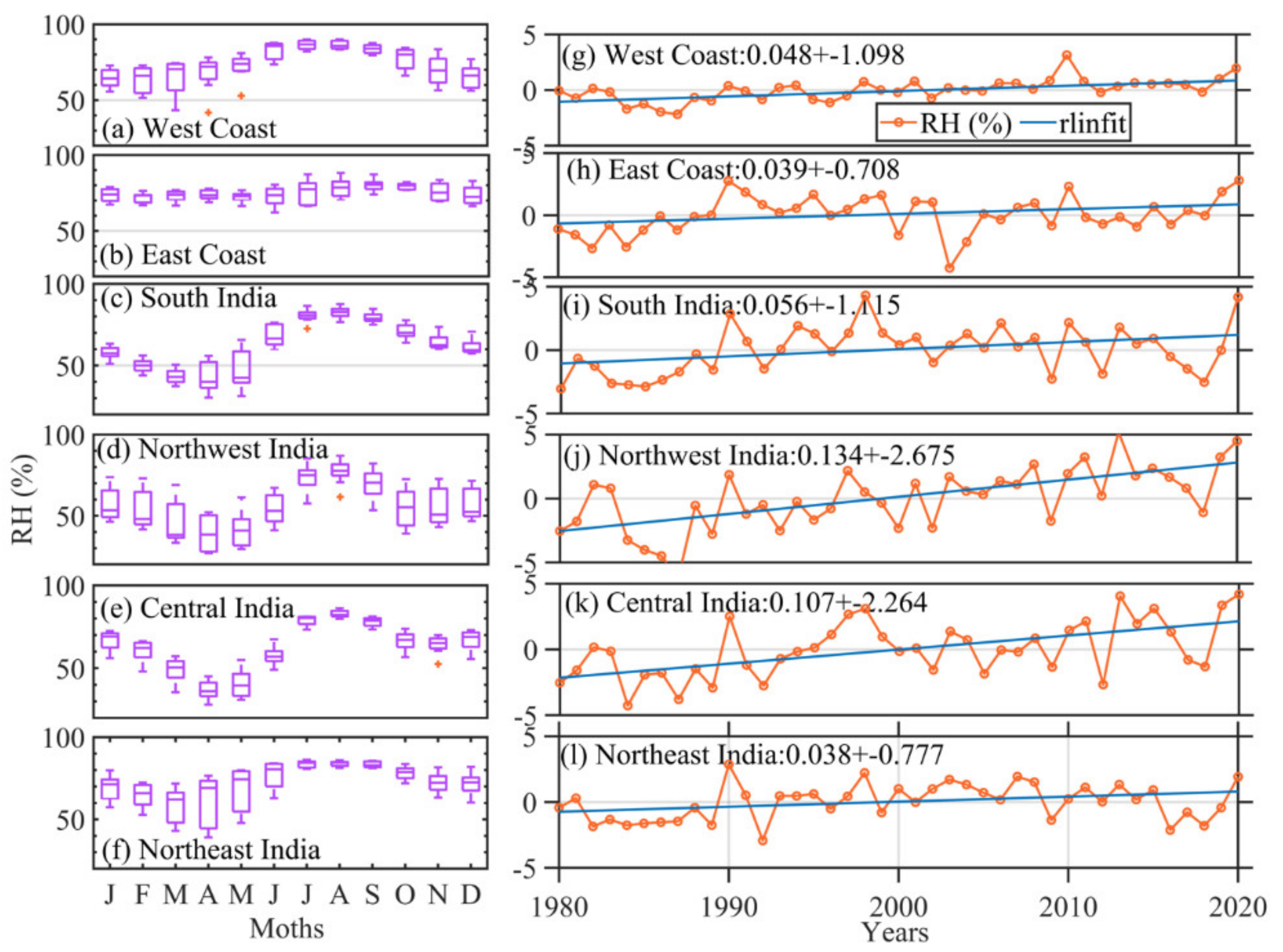
  • Relative humidity (RH) shows a large value in all stations except the Northwest stations during monsoon season, followed by post-monsoon season, and minimum in pre-monsoon season. The highest values are observed over the West Coast, followed by the East Coast and Northeast, and the minimum in Northwest in annual variability.
  • Monthly variation of RH over the East and West Coasts shows a different picture compared to other regions. The RH starts increasing from January and reaches a maximum during August and then decreases, whereas in other regions (South India, Northwest India, and Central India), the RH starts decreasing from January and reaches a minimum in April and again starts increasing and peaks to a maximum in August and later decreases.
  • An increase in RH during monsoons is noticed over central India. This increase in RH can be related to the increase in surface temperature. Northwest India shows a sharp increase in RH annually compared to other regions. This increase in surface RH might be due to the increase in vegetation over this region.
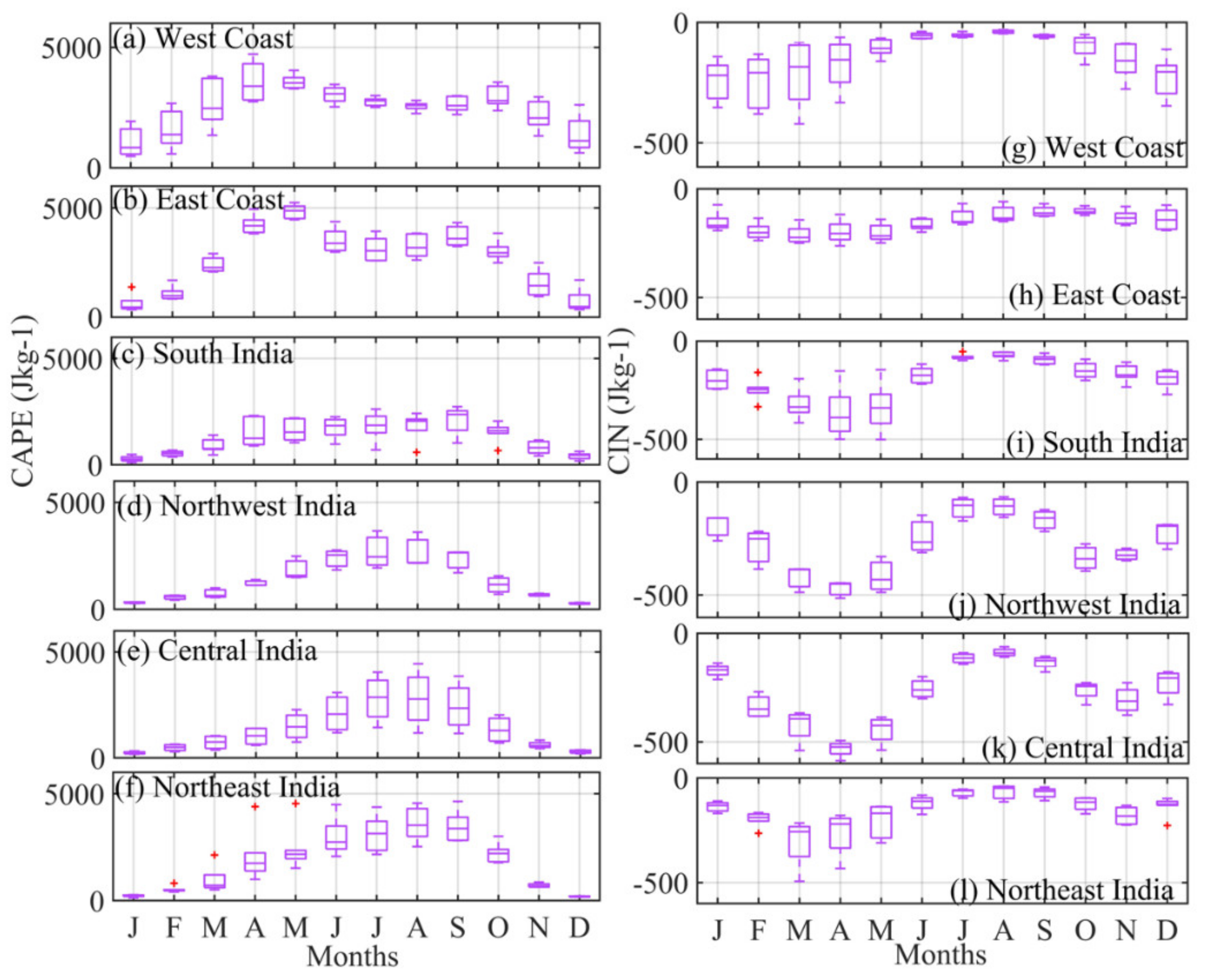
  • The highest values of Convective Available Potential Energy (CAPE) are observed over the West and East Coasts during pre-monsoon, monsoon, and post-monsoon seasons. Very low values are noticed during winter in the maximum number of stations. A completely opposite pattern is observed in Convective Inhibition (CIN) compared to CAPE variability, which is expected. The highest values of CAPE correspond to the lowest values of CIN and vice versa.
  • Region-wise viability of CAPE follows a similar pattern to RH. In West and East Coast stations, CAPE increases from January and attains a peak value during the month of May and decreases later, again reaching a maximum in September and decreasing thereafter. In these regions, during pre-monsoon season, instability conditions occur during severe land surface heating. In other regions, the increase in CAPE observed from January reaches a peak in August and decreases thereafter.
  • A significant increase in CAPE is observed over central India, followed by the East Coast region. The increase in moisture can lead to higher values of CAPE in these regions.

Author Contributions

Conceptualization, P.I.K.; methodology, P.I.K., G.B., P.P. and J.H.J.; formal analysis, P.K.; investigation D.V.R. and G.B.; resources, P.K.; data curation, P.I.K. and P.P.; supervision, M.V.R. and J.H.J.; writing—original draft, G.B.; writing—review and editing, R.S., M.V.R. and J.H.J. All authors have read and agreed to the published version of the manuscript.

Funding

Department of Electronics and Communications Engineering, Koneru Lakshmaiah Education Foundation, Vaddeswaram, Guntur, Andhra Pradesh, India.

Institutional Review Board Statement

Not applicable.

Informed Consent Statement

Not applicable.

Data Availability Statement

Publicly available datasets were analyzed in this study. National Climate Data Center and NCEP data center for providing hourly observations of surface data and radiosonde observations through IGRA.

Acknowledgments

Author J.H.J. acknowledges support from the Jet Propulsion Laboratory, California Institute of Technology, under contract with NASA.

Conflicts of Interest

The authors declare no conflict of interest.

References

  1. Jacob, D. The role of water vapour in the atmosphere. A short overview from a climate modeller’s point of view. Phys. Chem. Earth Part A Solid Earth Geod. 2001, 26, 523–527. [Google Scholar] [CrossRef]
  2. DeAngelis, A.M.; Qu, X.; Zelinka, M.D.; Hall, A. An observational radiative constraint on hydrologic cycle intensification. Nature 2015, 528, 249–253. [Google Scholar] [CrossRef] [PubMed]
  3. Ragi, A.R.; Sharan, M.; Haddad, Z.S. Investigation of WRF’s ability to simulate the monsoon-related seasonal variability in the thermodynamics and precipitation over southern peninsular India. Theor. Appl. Climatol. 2002, 141, 1025–1043. [Google Scholar] [CrossRef]
  4. Wagner, T.; Beirle, S.; Grzegorski, M.; Platt, U. Global trends (1996–2003) of total column precipitable water observed by Global Ozone Monitoring Experiment (GOME) on ERS-2 and their relation to near-surface temperature. J. Geophys. Res. 2006, 111, D12102. [Google Scholar] [CrossRef] [Green Version]
  5. Ahrens, C.; Samson, P. Extreme Weather and Climate, 1st ed.; Brooks Cole: Pacific Grove, CA, USA, 2011. [Google Scholar]
  6. IPCC. 2014 Summary for Policymakers. In Climate Change 2014: Impacts, Adaptation, and Vulnerability. Part A: Global and Sectoral Aspects; Contribution of Working Group II to the Fifth Assessment Report of the Intergovernmental Panel on Climate Change; Field, C.B., Barros, V.R., Eds.; Cambridge University Press: Cambridge, UK, 2014; pp. 1–32. [Google Scholar]
  7. Basha, G.; Kishore, P.; Venkat Ratnam, M.; Jayaraman, A.; Amir, A.K.; Taha, B.; Ouarda, M.J.; Velicogna, I. Historical and projected surface temperature over India during the 20th and 21st century. Nat. Sci. Rep. 2017, 7, 2987. [Google Scholar] [CrossRef] [Green Version]
  8. Maddu, R.; Vanga, A.R.; Sajja, J.K.; Basha, G.; Shaik, R. Prediction of land surface temperature of major coastal cities of India using bidirectional LSTM neural networks. J. Water Clim. Change 2021, 12, 3801–3819. [Google Scholar] [CrossRef]
  9. Dai, A. Recent climatology, variability, and trends in global surface humidity. J. Clim. 2006, 19, 3589–3606. [Google Scholar] [CrossRef] [Green Version]
  10. Bojinski, S.; Verstraete, M.; Peterson, T.C.; Richter, C.; Simmons, A.; Zemp, M. The concept of essential climate variables in support of climate research, applications, and policy. Bull. Amer. Meteor. Soc. 2014, 95, 1431–1443. [Google Scholar] [CrossRef]
  11. You, Q.L.; Min, J.Z.; Lin, N.H.B.; Pepin, N.; Sillanpää, M.; Kang, S.C. Observed climatology and trend in relative humidity in the central and eastern Tibetan Plateau. J. Geophys. Res. 2015, 120, 3610–3621. [Google Scholar] [CrossRef] [Green Version]
  12. Vicente-Serrano, S.M.; Azorin-Molina, C.; Sanchez-Lorenzo, A.; Morán-Tejeda, E.; Lorenzo-Lacruz, J.; Revuelto, J.; López-Moreno, J.I.; Espejo, F. Temporal evolution of surface humidity in Spain: Recent trends and possible physical mechanisms. Clim. Dyn. 2014, 42, 2655–2674. [Google Scholar] [CrossRef] [Green Version]
  13. Ross, R.J.; Elliott, W. Tropospheric water vapor climatology and trends over North America: 1973–1993. J. Climate 1996, 9, 3561–3574. [Google Scholar] [CrossRef] [Green Version]
  14. Ross, R.J.; Elliott, W. Radiosonde-based Northern Hemisphere tropospheric water vapor trends. J. Clim. 2001, 14, 1602–1612. [Google Scholar] [CrossRef]
  15. Zhai, P.; Eskridge, R.E. Atmospheric water vapor over China. J. Clim. 1997, 10, 2643–2652. [Google Scholar] [CrossRef]
  16. Bock, O.; Guichard, F.; Janicot, S.; Lafore, J.P.; Bouin, M.N.; Sultan, B. Multiscale analysis of precipitable water vapor over Africa from GPS data and ECMWF analyses, Geophys. Res. Lett. 2007, 34, L09705. [Google Scholar] [CrossRef] [Green Version]
  17. Zhao, T.; Dai, A.; Wang, J. Trends in tropospheric humidity from 1970 to 2008 over China from a homogenized radiosonde dataset. J. Clim. 2012, 25, 4549–4567. [Google Scholar] [CrossRef] [Green Version]
  18. Simmons, A.J.; Willett, K.M.; Jones, P.D.; Thorne, P.W.; Dee, D.P. Low-frequency variations in surface atmospheric humidity, temperature, and precipitation: Inferences from reanalyses and monthly gridded observational data sets. J. Geophys. Res. 2010, 115, D01110. [Google Scholar] [CrossRef]
  19. Brown, P.J.; DeGaetano, A.T. Trends in U.S. surface humidity, 1930–2010. J. Appl. Meteor. Climatol. 2013, 52, 147–163. [Google Scholar] [CrossRef]
  20. Basha, G.; Ratnam, M.V. Moisture variability over Indian monsoon regions observed using high resolution radiosonde measurements. Atmos. Res. 2013, 132–133, 35–45. [Google Scholar] [CrossRef]
  21. Basha, G.; Ratnam, M.V.; Krishna Murthy, B.V. Upper tropospheric water vapour variability over tropical latitudes observed using radiosonde and satellite measurements. J. Earth Sys. Sci. 2013, 122, 1583–1591. [Google Scholar] [CrossRef] [Green Version]
  22. Ratnam, M.V.; Basha, G.; Krishna Murthy, B.; Jayaraman, A. Relative humidity distribution from SAPHIR experiment onboard Megha-Tropiques satellite mission: Comparison with global radiosonde and other satellite and reanalysis datasets. J. Geophys. Res. 2013, 118, 9622–9630. [Google Scholar] [CrossRef]
  23. Basha, G.; Ratnam, M.V.; Kishore, P. Asian summer monsoon anticyclone: Trends and variability. Atmos. Chem. Phys. 2020, 20, 6789–6801. [Google Scholar] [CrossRef]
  24. Basha, G.; Ratnam, M.V.; Jiang, J.H.; Kishore, P.; Babu, S.R. Influence of Indian Summer Monsoon on Tropopause, Trace Gases and Aerosols in Asian Summer Monsoon Anticyclone Observed by COSMIC, MLS and CALIPSO. Remote Sens. 2021, 13, 3486. [Google Scholar] [CrossRef]
  25. Chen, J.; Dai, A.; Zhang, Y.; Rasmussen, K.L. Changes in convective available potential energy and convective inhibition under global warming. J. Clim. 2020, 33, 2025–2050. [Google Scholar] [CrossRef]
  26. Kishore, P.; Jyothi, S.; Basha, G.; Rao, S.V.B.; Rajeevan, M.; Velicogna, I.; Sutterley, T.C. Precipitation climatology over India: Validation with observations and reanalysis datasets and spatial trends. Clim. Dyn. 2016, 46, 541–556. [Google Scholar] [CrossRef] [Green Version]
  27. Meukaleuni, C.; Lenouo, A.; Monkam, D. Climatology of convective available potential energy (CAPE) in ERA-Interim reanalysis over West Africa. Atm. Sci. Let. 2016, 17, 65–70. [Google Scholar] [CrossRef] [Green Version]
  28. Durre, I.; Vose, R.S.; Wuertz, D.B. Overview of integrated global radiosonde archive. J. Climate 2006, 19, 53–68. [Google Scholar] [CrossRef] [Green Version]
  29. Basha, G.; Ratnam, M.V. Identification of atmospheric boundary layer height over a tropical station using high resolution radiosonde refractivity profiles: Comparison with GPS radio occultation measurements. J. Geophys. Res. 2009, 114, D16101. [Google Scholar] [CrossRef]
  30. Chakraborty, R.; Basha, G.; Ratnam, M.V. Diurnal and long-term variation of instability indices over a tropical region in India. Atmos. Res. 2018, 207, 145–154. [Google Scholar] [CrossRef]
  31. Chakraborty, R.; Ratnam, M.V.; Basha, S.G. Long-term trends of instability and associated parameters over the Indian region obtained using a radiosonde network, Atmos. Chem. Phys. 2019, 19, 3687–3705. [Google Scholar]
  32. Chakraborty, R.; Chakraborty, A.; Basha, G.; Ratnam, M.V. Lightning occurrences and intensity over the Indian region: Long-term trends and future projections. Atmos. Chem. Phys. 2021, 21, 11161–11177. [Google Scholar] [CrossRef]
  33. Kutner, M.; Nachsteim, C.J.; Neter, J. Applied Linear Regression Models, 4th ed.; McGraw-Hill: New York, NY, USA, 2014. [Google Scholar]
  34. Jaswal, A.K.; Koppar, A.L. Recent climatology and trends in surface humidity over India for 1969–2007. Mausam 2011, 62, 145–162. [Google Scholar] [CrossRef]
  35. Murugavel, P.; Pawar, S.D.; Gopalakrishnan, V. Trends of Convective Available Potential Energy over the Indian region and its effect on rainfall. Int. J. Climatol. 2012, 32, 1362–1372. [Google Scholar] [CrossRef]
  36. Gutzler, D.S. Climatic variability of temperature and humidity over the tropical western Pacific. Geophys. Res. Lett. 1992, 19, 1595–1598. [Google Scholar] [CrossRef]
  37. Gutzler, D.S. Low-frequency ocean-atmosphere variability across the tropical western Pacific. J. Atmos. Sci. 1996, 53, 2773–2785. [Google Scholar] [CrossRef] [Green Version]
  38. Gaffen, D.J.; Santer, B.D.; Boyle, J.S.; Christy, J.R.; Graham, N.E.; Ross, R.J. Multidecadal changes in the vertical temperature structure of the tropical atmosphere. Science 2000, 287, 1242–1245. [Google Scholar] [CrossRef]
  39. Gettelman, A.; Seidel, D.J.; Wheeler, M.C.; Ross, R.J. Multidecadal trends in tropical convective available potential energy. J. Geophys. Res. 2002, 107, 4606. [Google Scholar] [CrossRef]
  40. Brogniez, H.; Pierrehumbert, R.T. Using microwave observations to assess large-scale control of free tropospheric water vapor in the mid-latitudes. Geophys. Res. Lett. 2006, 33, L14801. [Google Scholar] [CrossRef] [Green Version]
  41. Khan, M.; Munoz-Arriola, F.; Rehana, S.; Greer, P. Spatial Heterogeneity of Temporal Shifts in Extreme Precipitation across India. J. Clim. Chan. 2019, 5, 19–31. [Google Scholar] [CrossRef]
Figure 1. Topographic map (based on ETOPO1 data provided by NOAA) over Indian subcontinent along with spatial distribution of 49 surface meteorological observations (empty circle) and 30 IMD radiosonde stations (filled circle) over 7 different geographic locations of India.
Atmosphere 13 00361 g001
Figure 2. The top panel (ae) shows the spatial distribution of the seasonal and annual mean relative humidity obtained from surface observational stations in India from 1980 to 2020. The bottom panel (fj) shows the spatial distribution of seasonal and annual trends in relative humidity.
Atmosphere 13 00361 g002
Figure 3. Box-whisker plots show composite monthly mean relative humidity over different regions in India (a) West coast (b) East coast (c) South India (d) Northwest India (e) Central India (f) Northeast India. (gl) represents region-wise averaged RH annual time series from 1980 to 2020. The blue line depicts the robust regression analysis performed at a 95% confidence interval to obtain the trend.
Atmosphere 13 00361 g003
Figure 4. The top panel (ae) shows the spatial distribution of the seasonal and annual mean Convective Available Potential Energy (CAPE) derived from radiosonde stations in India from 1980 to 2020. The bottom panel (fj) is the same as (ae) but for Convective Inhibition (CIN).
Atmosphere 13 00361 g004
Figure 5. The top panel (ae) shows the spatial distribution of seasonal and annual trends in Convective Available Potential Energy (CAPE) derived from radiosonde stations in India from 1980 to 2020. (fj) is the same as (ae) but for Convective Inhibition (CIN).
Atmosphere 13 00361 g005
Figure 6. (a) West Coast, (b) East Coast, (c) South India, (d) Northwest India, (e) Central India, and (f) Northeast India. (gl) is the same as (af) but for CIN.
Atmosphere 13 00361 g006
Figure 7. Time series of annual mean CAPE over different regions in India from 1980–2020. (a) West Coast, (b) East Coast, (c) South India, (d) Northwest India, (e) Central India, and (f) Northeast India. (gl) is the same as (af) but for CIN. The blue line depicts robust regression analysis performed at a 95% confidence interval to obtain the trend.
Atmosphere 13 00361 g007
Table 1. Location, mean sea level, seasonal, annual precipitation, and temperature values of different stations over India.
Station NameLatitudeLongitudeMSLWinterPre-MonsoonMonsoonPost-MonsoonAnnualWinterPre-MonsoonMonsoonPost-MonsoonAnnual
Precipitation (mm)Temperature (°C)
East coast
Kolkata22.6588.456.044.83221.20918.41426.131609.0120.9729.0029.5127.1926.69
Balasore21.5186.9318.846.97233.73909.01503.691693.2421.2329.6229.0526.4726.61
Bhubaneshwar20.2585.8345.037.59158.54901.06487.841585.0021.9529.3728.6126.3826.60
Vishakhapatnam17.6883.3069.935.91112.45445.82474.641068.8223.3929.5228.3926.5426.98
Machilipatnam16.2081.153.038.3374.53550.17478.151141.0324.9430.9830.0527.7128.44
Chennai13.0080.1813.7198.1263.64289.14693.0511239.0825.6231.0630.9928.1428.97
Karaikal10.9179.836.9326.21102.98194.00718.641327.7926.2030.7030.8928.4429.07
West Coast
Thiruvananthapuram8.4876.9559.9115.84311.42547.83606.041576.4626.2228.3126.6926.5226.94
Cochin9.9376.23170.59385.341634.82800.782889.9626.1528.3726.1326.2826.74
Mangalore12.9574.8330.821.43223.722953.78698.843897.6024.3527.1023.9924.7025.04
Goa15.4873.8158.46.8568.953041.42533.853650.8425.2028.6026.2426.5426.65
Ratnagiri16.9873.3390.54.8950.162631.87549.743236.6525.2428.8526.4726.7226.82
Pune18.5373.85555.06.2023.40849.90300.581179.9523.3528.4125.9425.7225.86
Bombay19.1172.8514.23.7515.762272.47485.722777.6923.3028.7027.2626.6126.48
Surat21.2072.8310.02.993.531088.96243.431338.9022.7430.4829.5227.9227.68
Ahmadabad23.0672.6355.02.946.26649.21132.64791.0619.6729.4328.8726.0826.04
Northwest India
Bhuj rudramata23.2569.8078.02.834.10356.0391.00453.8421.5528.8829.7127.6526.96
Udaipur24.6173.88509.06.6614.17526.84109.32657.0118.3828.9828.6425.3525.37
Jodhpur26.3073.01217.07.0423.82276.2453.41360.5217.5829.5730.8826.1726.09
Jaipur26.8175.80383.016.9026.19461.1590.46594.7216.9529.2230.7725.7825.72
Bikaner28.0073.30223.012.6334.92212.3739.79299.7016.5229.0632.0626.2826.02
New Delhi28.5877.20211.036.6144.91395.48106.20583.1915.3627.8631.2825.2424.97
Patiala30.3376.46251.073.6670.38521.68137.23802.7613.3024.5128.8922.7222.39
Dehradun30.3178.03683.0130.32146.39887.44211.661375.6111.7521.6325.1820.0919.69
West Himalayas
Srinagar34.0874.831585.0269.25363.18247.15141.751020.446.1516.1123.8616.3715.66
Central India
Bareilly28.3679.40167.044.6542.48641.98185.53914.6514.9326.2029.0823.8423.55
Gorakhpur26.7583.3678.329.1856.59778.23251.981115.9817.0528.1830.1325.8225.33
Agra27.1577.96168.022.7924.98442.07114.74604.6015.7728.6831.6225.5625.45
Gwalior26.2378.25205.026.7520.50536.70159.99743.7216.4629.6631.3725.7425.85
Allahabad25.4581.7398.033.2122.54589.21215.72860.7017.2229.3230.5625.6025.71
Bhopal23.2877.35522.029.5317.57889.76206.651143.4718.5529.8328.2324.6025.33
Jabalpur23.2079.95397.044.3326.82914.66231.091216.7418.1629.4228.1524.2625.03
Jamshedpur22.8186.18142.038.89145.31866.71327.901378.7220.3229.8729.3726.2326.48
Lucknow26.7580.88122.035.9130.59564.56209.19840.2316.8228.7830.5525.6325.48
Northeast
Jharsiguda21.9184.08228.039.3275.94997.54292.651405.3720.6130.2328.3025.3026.14
Patna25.6085.1651.024.2069.94707.83246.971048.9517.5128.0329.8925.9525.38
Gaya24.7584.95116.028.5451.59699.44250.421029.9817.2928.4429.4225.0625.09
Ranchi23.3185.31646.035.0391.59779.91294.581201.0818.5628.7728.4424.8025.17
Dibrugarh27.4895.01110.089.88614.081190.24406.772300.4617.9524.2228.5425.3124.02
Guwahati26.1091.5854.040.48479.521037.38395.101951.6416.9123.6327.3824.1923.05
Imphal24.7693.90781.055.00382.72749.16331.331517.7817.2023.8126.9224.2423.06
Agartala23.8891.2516.032.30460.19726.45298.521516.9017.3824.2426.9224.2923.22
South India
Nagpur21.1079.05310.034.8533.08818.34224.971110.4519.9730.1427.6724.5825.62
Raipur21.2381.65296.022.4836.74834.62246.461140.2619.7130.0028.4025.0025.81
Aurangabad19.8575.40585.011.0220.32431.29233.01695.2522.2130.4127.2025.2626.29
Jagdalpur19.0882.03554.019.35123.111048.24361.931552.6621.9329.8527.6825.4926.26
Hyderabad17.4578.46530.016.3167.56447.76276.54808.0123.6931.5028.0825.9627.33
Bangalore12.9677.58917.022.76158.23249.71369.58799.8423.1828.2325.8724.6725.50
Gadag15.4175.63670.011.85100.60259.34244.078615.6324.1429.1625.7425.4026.12
Publisher’s Note: MDPI stays neutral with regard to jurisdictional claims in published maps and institutional affiliations.

