Article

Impact of Wildfires on Meteorology and Air Quality (PM2.5 and O3) over Western United States during September 2017

by
Amit Sharma
1,2,*,
Ana Carla Fernandez Valdes
1 and
Yunha Lee
1,3,4,*
1
Laboratory for Atmospheric Research, Department of Civil and Environmental Engineering, Washington State University, Pullman, WA 99164, USA
2
Department of Civil and Infrastructure Engineering, Indian Institute of Technology Jodhpur, Rajasthan 342030, India
3
Center for Advanced Systems Understanding (CASUS), 02826 Gorlitz, Germany
4
Helmholtz-Zentrum Dresden Rossendorf (HZDR), 01328 Dresden, Germany
*
Authors to whom correspondence should be addressed.
Atmosphere 2022, 13(2), 262; https://doi.org/10.3390/atmos13020262
Submission received: 27 December 2021 / Revised: 28 January 2022 / Accepted: 29 January 2022 / Published: 3 February 2022
(This article belongs to the Special Issue Feature Papers in Atmosphere Science)

Abstract

:
In this study, we investigated the impact of wildfires on meteorology and air quality (PM2.5 and O3) over the western United States during the September 2017 period. This is done by using Weather Research and Forecasting model coupled with Chemistry (WRF-Chem) to simulate scenarios with wildfires (base case) and without wildfires (sensitivity case). Our analysis performed during the first half of September 2017 (when wildfire activity was more intense) reveals a reduction in modelled daytime average shortwave surface downward radiation especially in locations close to wildfires by up to 50 W m−2, thus resulting in the reduction of the diurnal average surface temperature by up to 0.5 °C and the planetary boundary layer height by up to 50 m. These changes are mainly attributed to aerosol-meteorology feedbacks that affect radiation and clouds. The model results also show mostly enhancements for diurnally averaged cloud optical depth (COD) by up to 10 units in the northern domain due to the wildfire-related air quality. These changes occur mostly in response to aerosol–cloud interactions. Analysis of the impact of wildfires on chemical species shows large changes in daily mean PM2.5 concentrations (exceeding by 200 μg m−3 in locations close to wildfires). The 24 h average surface ozone mixing ratios also increase in response to wildfires by up to 15 ppbv. The results show that the changes in PM2.5 and ozone occur not just due to wildfire emissions directly but also in response to changes in meteorology, indicating the importance of including aerosol-meteorology feedbacks, especially during poor air quality events.

1. Introduction

Wildfires in North America degrade air quality not just at locations in the vicinity of the fire activity but also in remote downwind regions due to long-range transport of smoke plumes [1,2,3,4]. In addition, wildfires can also perturb meteorology through impacts of air pollutants on meteorology such as aerosol-radiation and aerosol–cloud interactions [5]. Aerosols interact with the incoming solar radiation directly by scattering and absorbing and thus altering Earth’s radiative balance [6,7]. Aerosols can also interact with clouds to change their microphysical properties (and thus lifetime) by acting as cloud condensation nuclei (CCN) [8,9].
Historically, large wildfires over western United States (US) have been shown to increase in frequency and duration after the mid-1980s with the greatest changes associated with increased spring and summer temperatures possibly caused by reduced winter precipitation together with earlier spring snowmelt [10]. The observed trend in area burned due to wildfires in the western US has also been notably attributed to declining trends in summer precipitation during the past few decades [11] which has been further linked to the declining Arctic sea-ice extent [12]. The burned area over the western US is further projected to increase by 54% in 2046–2055 relative to 1996–2005 due to climate change [13]. Such an increase in wildfire activity can be expected to enhance impacts on air quality and meteorology in the future.
Several research studies have reported the contribution of wildfires to different pollutants like PM2.5, O3, NO2 and CO [14,15,16,17,18,19,20,21]. Mallia et al. [14] analyzed the impacts of intense episodes during the 2007 and 2012 wildfire seasons on Salt Lake City, a downwind urban center, using the Stochastic Time-Inverted Lagrangian Transport (STILT) model. The study reported an enhancement of 15 µg/m3 in 24 h average PM2.5 over the city. Lu et al. [15] used a statistical model to simulate ozone enhancements by wildfires and found an increase of about 10–20 ppbv in summer mean MDA8 (daily maximum 8 h average) ozone at sites in Intermountain West. Wilkins et al. [17] used the Community Multiscale Air Quality (CMAQ) modelling system over the contiguous US and reported a wildfire contribution of 11% to mean PM2.5 and less than 1% to mean O3 concentrations during 2008–2012. Zhang et al. [21] analyzed the impacts of duff and peat consumption during wildfires in the southeastern United States using a regional air quality model and found an increase of about 61.3% over a region about 300 km within the fire location.
While the adverse impacts of wildfires on air quality and human health have been explored in several studies for both present-day [4,22,23,24,25,26] and future scenarios [27], the role of aerosols, originating from wildfire emissions particularly over the western US, in perturbing meteorology is relatively less explored [28]. In this study, we use the Weather Research and Forecasting model coupled with chemistry (WRF-Chem), an “online” meteorology–chemistry coupled model [29,30,31,32,33], to investigate the impact of wildfire emissions on meteorology and air quality (PM2.5 and O3) over the western US while considering aerosol–cloud–radiation interactions in the model.
WRF-Chem has been used in several studies focused on wildfires or biomass burning episodes over different regions [5,28,34,35]. Grell et al. [35] simulated the 2004 Alaskan wildfires to show that the inclusion of wildfires in the model simulations improved in comparison with the soundings. The study also reported significant modifications of vertical profiles of temperature and moisture in cloud-free areas. Jiang et al. [28] analyzed the impact of wildfires over the western US on radiation, meteorology and ozone photochemistry. The study reported a reduction in downward solar radiation reaching the surface, temperature near surface and photolysis rates by up to 50 W m−2, 2 K and 75%, respectively, along with reductions in biogenic isoprene emissions. The study concluded that incorporating radiative impacts of wildfire-related aerosols may reduce ozone overestimation generally seen in the traditional photochemical models that do not consider aerosol–meteorology feedbacks. Archer-Nicholls et al. [5] reported a net cooling (−4.08 ± 1.53 W m−2) averaged for three 36 h biomass burning case studies over Brazil in September 2012 associated with direct aerosol–radiation interaction due to aerosols from biomass burning.
In this study, we investigate the impact of the September 2017 wildfires over the western US, which showed some of the most intense wildfire activity in recent years over this region, on air quality and meteorology. The current study is arranged as follows: Section 2 presents the WRF-Chem configuration used in this study including domain information, physics and chemistry options, initial and boundary conditions, input emissions and observation data used for model evaluation. We present the results in Section 3 by dividing them into two subsections: (a) model evaluation against surface measurements and satellite data, and (b) sensitivity results analysis including the impact of wildfires on radiation, meteorology, cloud, CCN activity, surface pollutant levels and PM2.5 chemical composition. Finally, the summary and conclusions of the study are presented in Section 4.

2. Materials and Methods
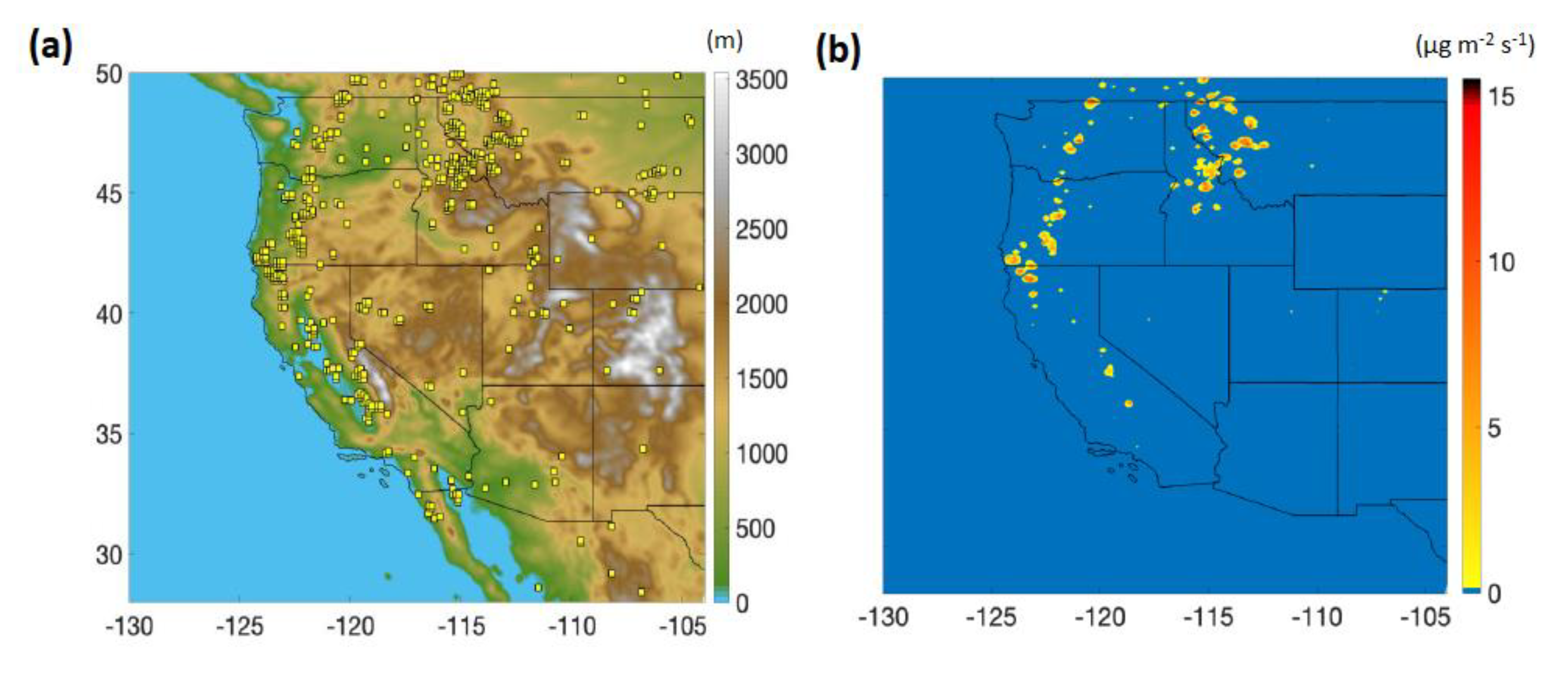
2.1. Model Domain

We used WRF-Chem version 3.9.1.1 (https://www2.mmm.ucar.edu/wrf/users/download/get_sources.html#current; accessed on 15 January 2022) to simulate the wildfire period during September 2017 over the western US. Figure 1a shows the model domain and terrain height along with wildfire impacted locations during September 2017. The domain is set using lambert projection and is centered at 38° N, 121° W with 279 grid points in both the east-west and north-south directions. The spatial resolution is 12 km × 12 km in the horizontal direction along with 32 vertical levels from the surface up to 50 hPa pressure level. Moderate Resolution Imaging Spectroradiometer (MODIS) land-use dataset [36,37] is used to define model terrain type.

2.2. Model Physics and Meteorological Initial and Boundary Conditions

The cloud microphysics in the model is based on the Morrison double-moment scheme [38], and the cumulus convection is based on the Grell-Freitas scale and aerosol aware convection scheme [39]. Rapid Radiative Transfer Model (RRTM) longwave scheme [40] and Goddard shortwave scheme [41] were used to represent the radiative transfer in the model. Surface physics is based on the unified Noah land surface model [42] along with the ETA similarity option [43,44,45]. The planetary boundary layer (PBL) physics is based on the Bougeault and Lacarrere (BouLac) PBL scheme [46]. The Global Forecast System (GFS) analysis dataset (www.ncdc.noaa.gov/data-access/model-data/model-datasets/global-forcast-system-gfs/; accessed on 31 January 2022), available at 6 h temporal and 0.5° horizontal resolution, was used to provide initial and lateral boundary conditions for meteorology.

2.3. Model Chemistry and Chemical Initial and Boundary Conditions

We used Model for Ozone and Related Chemical Tracers (MOZART) gas phase chemistry [47] along with Model for Simulating Aerosol Interactions with Chemistry (MOSAIC) 4-bin aerosol scheme [48] in this study. The MOSAIC aerosol scheme includes a volatility basis set (VBS) for secondary organic aerosols (SOA). The photolysis rate calculations are based on the Madronich photolysis scheme [49]. The gas dry deposition process in the model is represented by the resistance in the series approach from Wesely [50]. Aerosol–radiation and aerosol–cloud interactions are turned on to account for aerosol–meteorology feedbacks. Aerosol optical properties are calculated using volume approximation. The chemical initial and lateral boundary conditions are prepared using MOZART-4/GEOS5 output available at 6 h temporal resolution (https://www.acom.ucar.edu/wrf-chem/mozart.shtml; last accessed on 31 January 2022).

2.4. Emission Inputs

Hourly anthropogenic emissions for the study were generated using the 2014 National Emissions Inventory (NEI) (https://www.epa.gov/air-emissions-inventories/2014-national-emissions-inventory-nei-data; last accessed on 31 January 2022). The biogenic emissions were prepared using the Model of Emissions of Gases and Aerosols from Nature (MEGAN) modeling system [51]. Furthermore, hourly wildfire emissions were prepared using the Fire Inventory from NCAR (FINN) version 1.0 [52]. Figure 1a shows the wildfire impacted locations derived from the FINN dataset over the western US in September 2017. The intensity of these wildfires is further depicted in Figure 1b in terms of PM2.5 emissions from fire activity, which reveals that the major fires occurred in several locations in the north-western US (in states of Washington, Idaho, Montana and Oregon) with some incidences in other states (e.g., California). PM2.5 emission flux in some of the major fires reached up to 15 µg m−2 s−1.

2.5. Simulation Details

Two simulations were carried out in this study: a base run with wildfire emissions included (called ‘Fire’ simulation hereafter) and another run without wildfire emissions (called ‘noFire’ simulation hereafter). Both simulations are run from 28 August 2017 to 1 October 2017 at a time step of 60 s with the first 4 days of the model output discarded as spin up period. The output of the model was generated and stored every hour for analysis.

2.6. Observational Datasets for Model Evaluation

We used surface measurements from the U.S. Environmental Protection Agency (USEPA, Washington, DC, USA) Air Quality System (AQS; https://www.epa.gov/aqs, accessed on 14 February 2021) for meteorological variables (air temperature at 2 m and wind speed at 10 m) and chemical species (PM2.5 and O3). The measurements for Air Quality System (AQS) are made at locations maintained by the USEPA, state, local and tribal agencies [19]. The observations are made at both urban as well as rural locations using diverse techniques (https://aqs.epa.gov/aqsweb/documents/codetables/methods_met.html; accessed on 22 January 2022). Some of the techniques are:
(1)
PM2.5—Gravimetric and beta-attenuation technique;
(2)
O3—Chemiluminescence and UV Photometry;
(3)
Surface temperature—Thermo Electron Model RAAS2.5-200 Audit w/VSCC and R & P Model 2000 PM-2.5 FEM Air Sampler;
(4)
Wind speed—Vaisala WS425 and Met One Sonic Anemometer Model 50.5.
The data are quality-assured before being sent to EPA AQS (https://aqs.epa.gov/aqsweb/documents/about_aqs_data.html; last accessed on 22 January 2022). Data from Moderate Resolution Imaging Spectroradiometer (MODIS) on board NASA’s Terra satellite [53] are also used in this study to evaluate the model output for variables such as monthly average shortwave surface downward radiation (SSDR), outgoing longwave radiation (OLR) at the top of the atmosphere (TOA), cloud fraction and cloud optical depth (COD): the data were obtained from https://neo.sci.gsfc.nasa.gov (accessed on 14 February 2021). The spatial resolution of the MODIS data used in this study was 0.5°. WRF-Chem data were compared with MODIS data at approximate overpass time of Terra satellite (1900 UTC) and with Modern-Era Retrospective analysis for Research and Applications, version 2 (MERRA-2) model [54] data (diurnal average) over the western US during September 2017. AOD data for the Terra satellite and MERRA-2 model were obtained from https://giovanni.gsfc.nasa.gov/giovanni/ (accessed on 14 February 2021).

3. Results and Discussion

3.1. Evaluation of the Base run

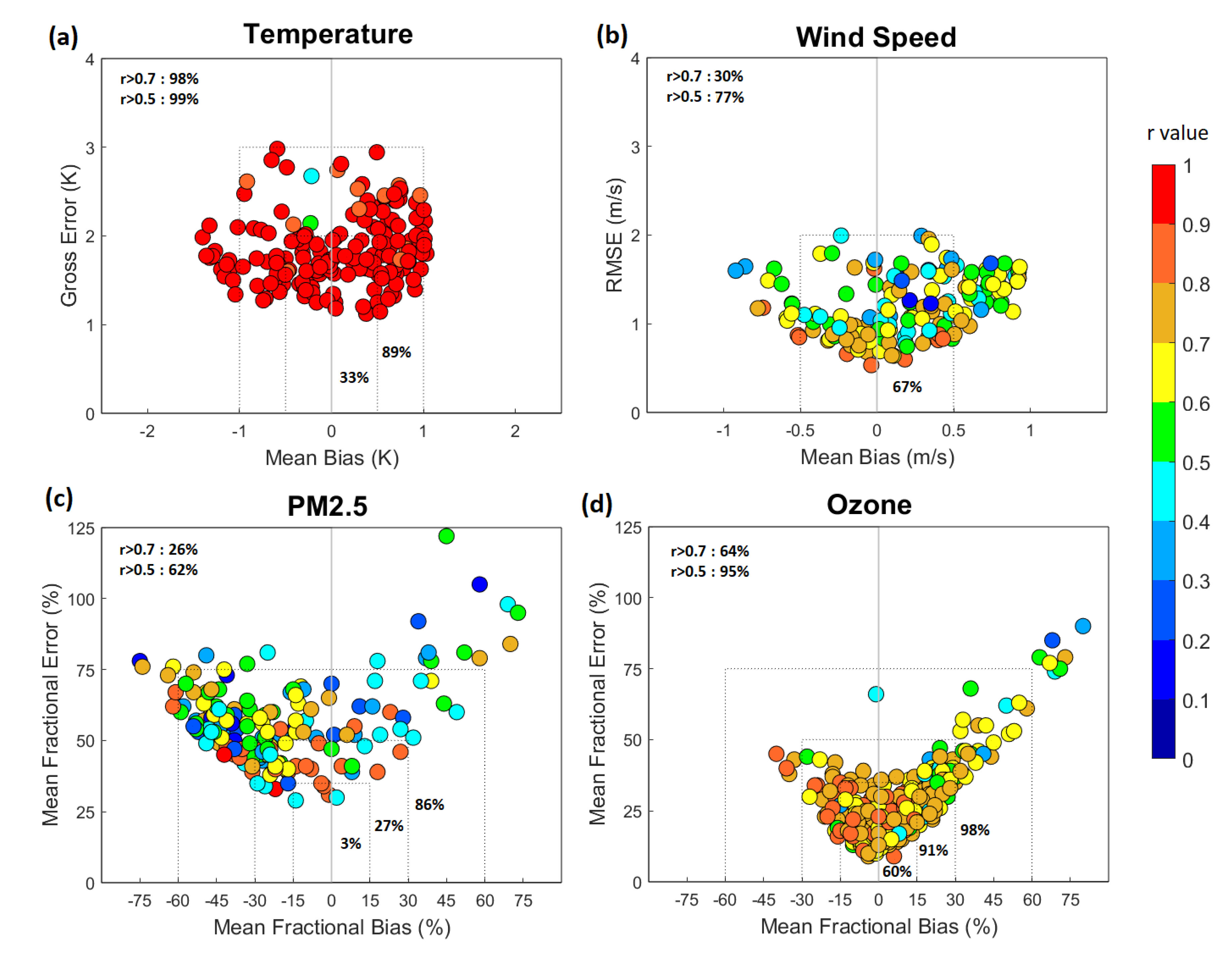
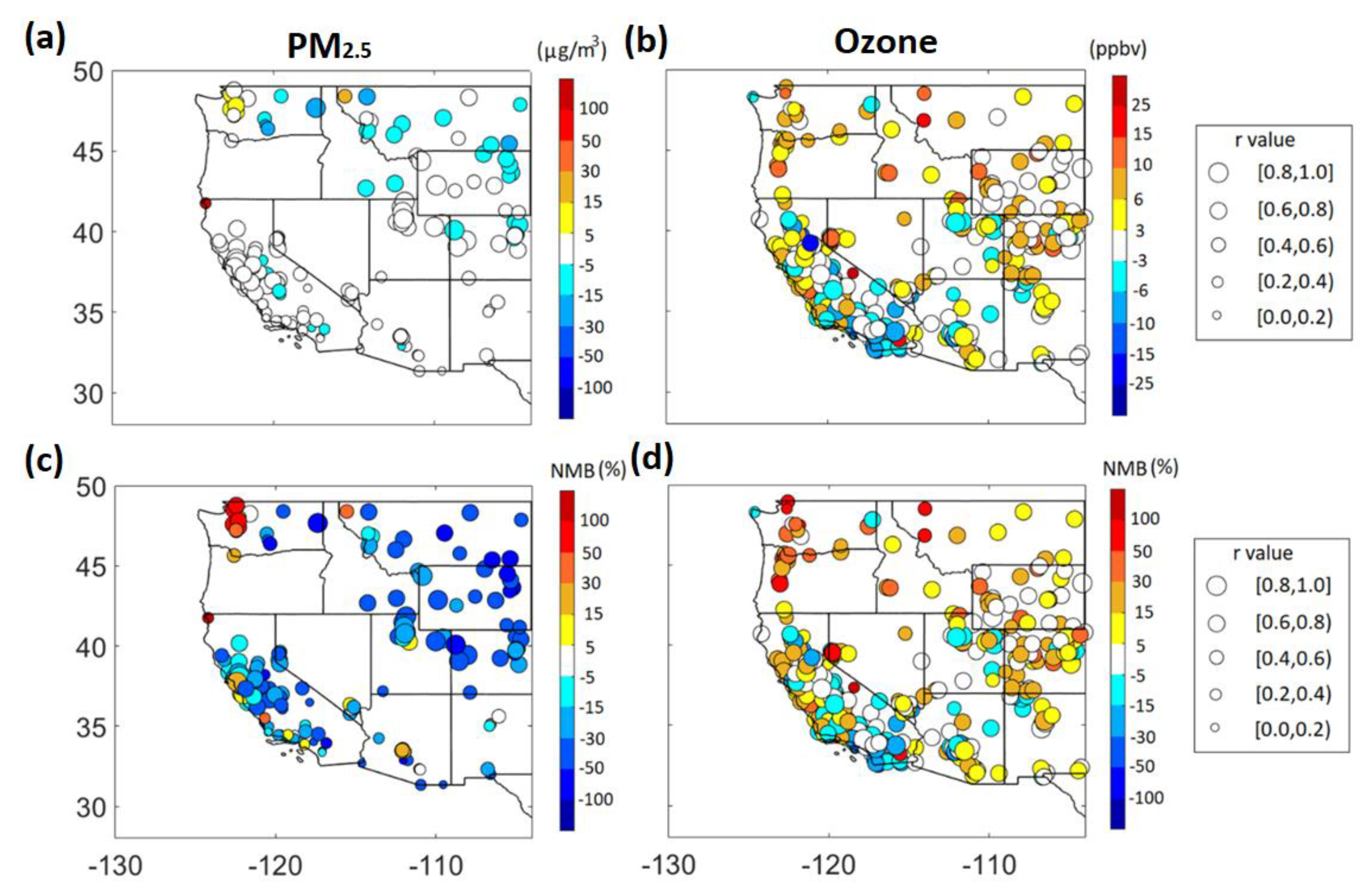
3.1.1. Evaluation against Surface Measurements

Figure 2 shows model performance for hourly outputs when evaluated against AQS measurements available over the domain for the month of September 2017 using soccer plots (https://www.epa.gov/cmaq/atmospheric-model-evaluation-tool; accessed on 14 February 2021). The soccer plots summarize the model performance by depicting goals and criteria lines. We follow benchmarks adopted in Zhang et al. [55] for 2 m temperature (Mean bias within ±1.0 K and gross error < 3 K) and 10 m wind speed (Mean bias within ±0.5 m s−1 and root mean square error < 2 m s−1). For PM2.5 and ozone, we follow the benchmark used in Morris et al. [56], although only for PM2.5 constituents, with plots depicting model performance based on the mean fractional bias (MFB in %) and mean fractional error (MFE in %) values at the available measurement stations. The model performance is categorized as excellent (|MFB| ≤ 15%, MFE ≤ 35%), good (|MFB| ≤ 30%, MFE ≤ 50%), average (|MFB| ≤ 60%, MFE ≤ 75%) and needing improvement (|MFB| ≥ 60%, MFE ≥ 75%) [57]. Figure 2 also shows correlation coefficient (r) values on color scale from 0 to 1.
Figure 2a shows the model performance for 2 m temperature (°C). The model performs within recommended performance criteria at 89% of stations. The correlation coefficient value is greater than 0.5 (0.7) at 99% (98%) of stations, establishing the model’s ability to capture hourly variations in near-surface temperature quite well. For 10 m wind speed (m/s) in Figure 2b, the model performs within the recommended performance criteria at 67% of stations. The poor performance for wind speed at several stations is possibly due to the model’s inability to adequately resolve topography even at 12 km resolution. The correlation coefficient value for wind speed is greater than 0.5 (0.7) at 77% (30%) of the stations.
For surface PM2.5 concentration (µg m3) shown in Figure 2c, the model’s performance is excellent at only 3% of stations, good at 24% of stations, average at 59% of stations and poor at the remaining 14% of stations. The poor performance at some stations may be attributed to several factors including model resolution and uncertainty in emissions. The correlation coefficient value for PM2.5 is greater than 0.5 (0.7) at 62% (26%) of stations. Finally, Figure 2d shows the model performance for surface O3 mixing ratios (ppbv). Model performance is excellent at 60% of stations, good at 31% of stations, average at 7% of stations and poor at only 2% of stations. The correlation coefficient value for O3 is greater than 0.5 (0.7) at 95% (64%) of stations, indicating an overall reasonably good model performance for O3 over the domain. We also show the spatial distribution of the model’s performance (r and MB/NMB) for PM2.5 and O3 in Figure 3. Stations exhibiting noticeable positive bias for PM2.5 (MB ≥ 5 µg m−3; NMB ≥ 15%) lie in western Washington, the coastal boundary of Oregon and California and a station in western Montana (Figure 3a,c), locations which lie in the vicinity of wildfire impacted regions, indicating possible uncertainty in wildfire emissions and the vertical plume distribution in the model. The model seems to compensate for the overestimation at the above-mentioned locations by underestimating PM2.5 at other stations in the vicinity of wildfire impacted locations (e.g., eastern Washington). The model also overestimates PM2.5 in some coastal locations in California (though MB is within ±5 µg m−3) and a few stations inland (e.g., some locations in Arizona, Utah and Nevada). At the remaining stations, the model mostly tends to underpredict the PM2.5 concentrations possibly due to several reasons including uncertainty in wildfire and anthropogenic emissions and due to the fact that the NEI inventory used in this study is representative of the year 2014. The anthropogenic emissions of most criteria pollutants in 2017 were less than those in 2014 (https://www.epa.gov/sites/production/files/2020-04/documents/nei2017_tsd_full_30apr2020.pdf; last accessed on 31 January 2022). For ground-level ozone, the model generally overpredicts in the vicinity of the wildfires with NMB > 30% at some of the locations (Figure 3b, d). At the other locations throughout the domain, NMB is mostly within ±30%.

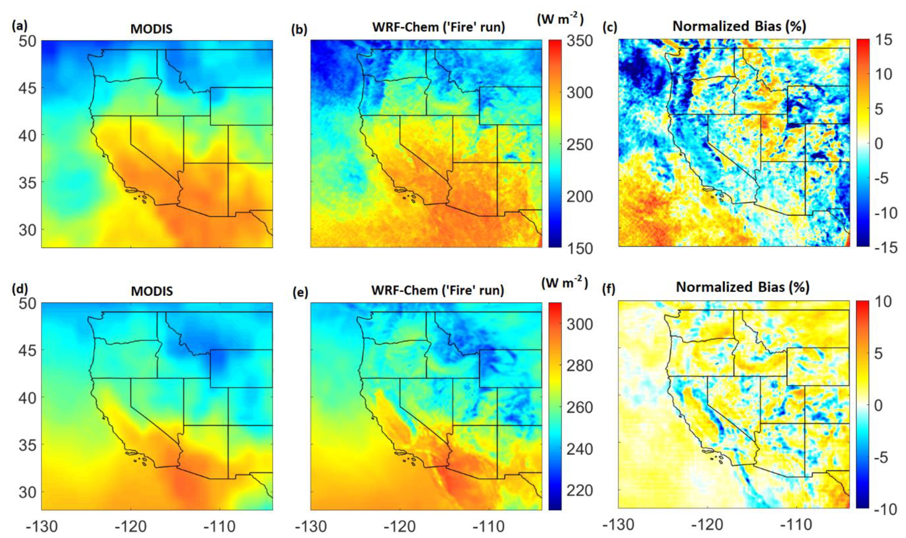
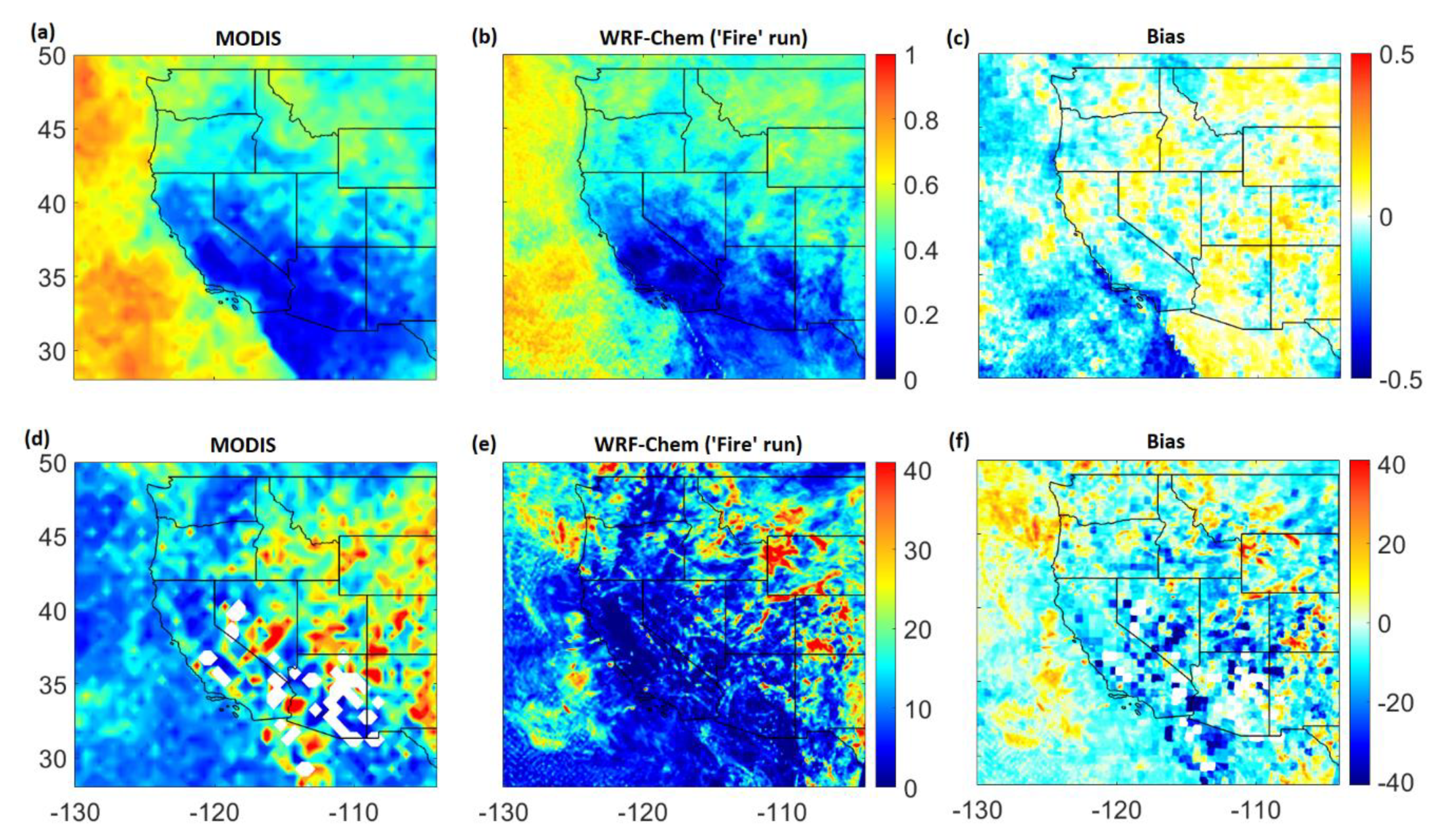
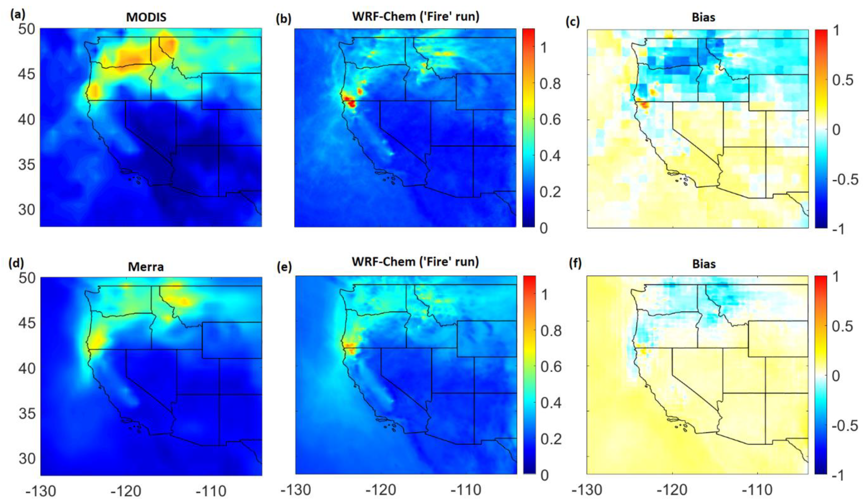
3.1.2. Evaluation against Satellite Measurements

We evaluated key variables, which are used for sensitivity analyses later in this study, against satellite measurements. Figure 4 shows the comparison of SSDR and OLR from WRF-Chem ‘Fire’ run and MODIS data. The model captures the spatial distribution of averaged SSDR and OLR for satellite overpass times quite well with higher SSDR/OLR in the southern regions compared to northern regions. The spatial correlation coefficient between the model and MODIS for SSDR is 0.92 with a mean bias of −0.65 W m−2 (NMB of ~−0.3%) over the domain. Similarly, the spatial correlation coefficient between the model and MODIS for OLR is 0.96 with a mean bias of 4.7 W m−2 (NMB of ~1.8%).
Next, we show the model comparison for cloud fraction and cloud optical depth (COD) in Figure 5. The model cloud fraction is in good agreement qualitatively with the MODIS cloud fraction, although the model underpredicts especially over the ocean region. The spatial correlation coefficient between the model and MODIS for cloud fraction is 0.70 with a mean bias of −0.10 (NMB of ~−18%) over the domain. The negative bias is primarily attributed to the underprediction of cloud cover over the ocean region. The model captures COD reasonably well in north and eastern regions but tends to underpredict in other areas (south-west) over the western US. This is possibly due to missing satellite data for COD in some regions on several days for the analysis period as seen in daily satellite outputs (not shown here), and hence model statistics are not presented for COD.
We also present a comparison of WRF-Chem AOD with MODIS and MERRA-2 global model AOD in Figure 6. AOD comparison between WRF-Chem and MODIS in Figure 6a,b reveals noticeable differences. For example, WRF-Chem shows high AOD as compared to MODIS AOD in south-west Oregon and north-west California regions. Both model and MODIS AODs are elevated in some regions like eastern Washington, most of Idaho and western Montana, but the model AOD is generally much smaller than the MODIS AOD in these regions. The reason for the AOD mismatch between model and MODIS can be attributed to several reasons including uncertainty in wildfire emissions and vertical plume distribution in the model. Nevertheless, the model evaluation statistics are found to be reasonable (r = 0.72; MB = −0.04; NMB = −20%). We also present the WRF-Chem evaluation with MERRA-2 global model data (Figure 6d,e). Both WRF-Chem and MERRA-2 models agree qualitatively with a similar spatial variation of AOD in the locations lying in the vicinity of the wildfires (e.g., south-west Oregon and north-west California). However, compared to MERRA-2, WRF-Chem shows higher AOD over south-west Oregon, north-west California and over marine regions and lower AOD over other wildfire impacted locations inland (e.g., western Montana). The differences in AOD between the WRF-Chem and MERRA-2 models might arise due to several reasons including relatively coarse resolution of the latter (0.5° × 0.625°) and differences in the fire inventory used. The MERRA-2 model uses Quick Fire Emissions Dataset (QFED) for biomass burning emissions of carbonaceous and sulfate aerosols [57]. Statistically, WRF-Chem performs reasonably well when compared to MERRA-2 AOD (r = 0.85; MB = 0.01; NMB = 3%).

3.2. Sensitivity Analysis: Impact of Wildfires

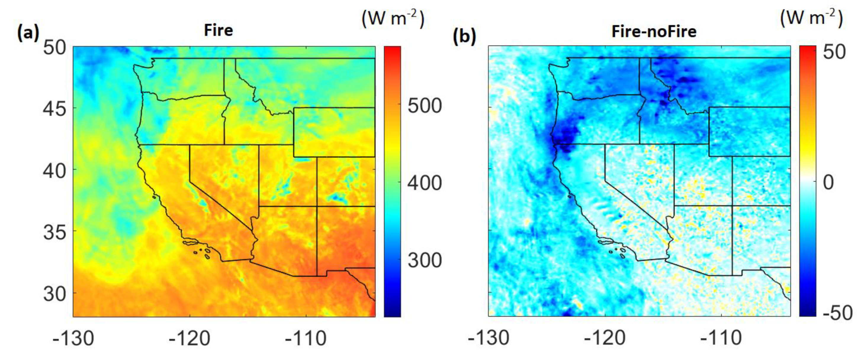
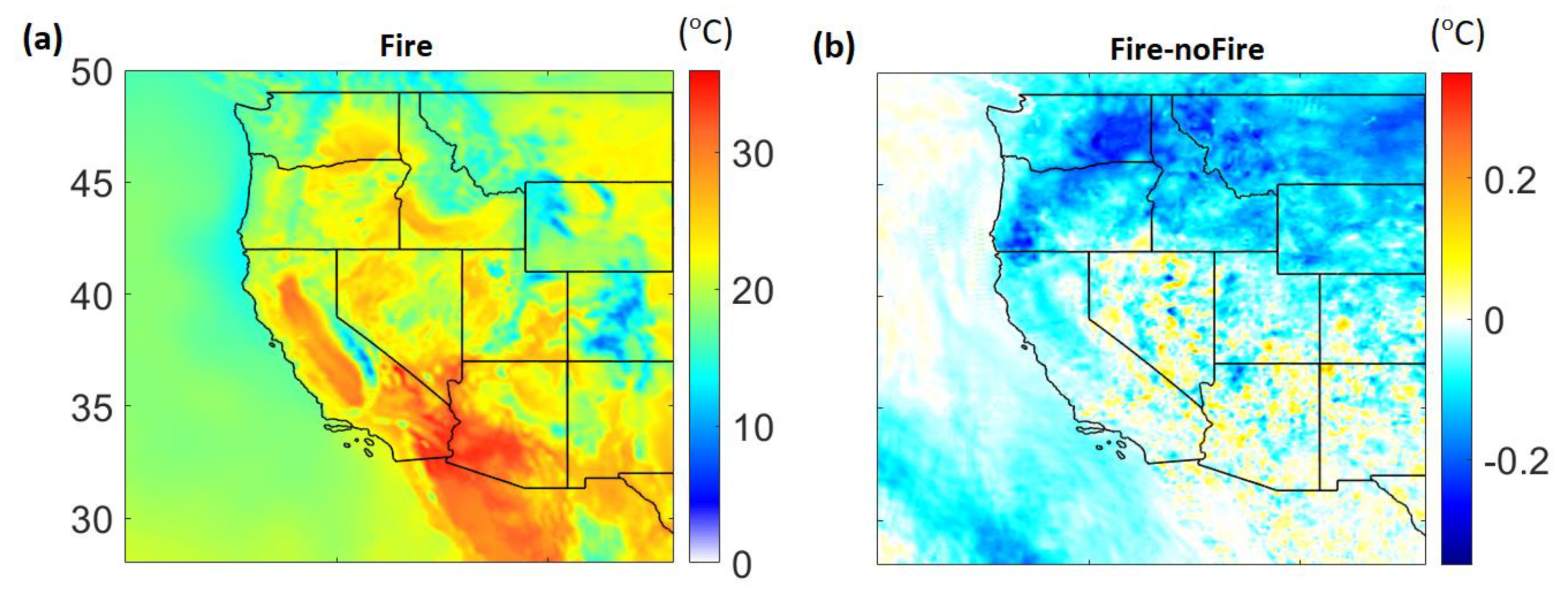
3.2.1. Impact on Surface Shortwave Radiation and Meteorology

Given the reasonable model performance against surface observations and satellite measurements, here we present the impact of wildfires by comparing ‘Fire’ and ‘noFire’ simulations. The following comparison is carried out only for first the half of September 2017 during which fire activity was relatively intense. Figure 7 shows the impact of wildfires on daytime average (0600-1700 IST) SSDR during the first half of September 2017. Figure 7a shows the daytime average radiation in the ‘Fire’ simulation whereas Figure 7b shows the differences between the daytime average radiation from ‘Fire’ and ‘noFire’ simulations. The average shortwave radiation reduces in the north and over the coastal regions because of aerosol–radiation–cloud interactions due to the wildfires. The reduction is up to 50 W m−2 in some locations in the vicinity of the wildfires. Analysis of maximum change over the diurnal scale reveals the reduction of more than 100 Wm−2 over the same regions (not shown).
Figure 8 shows the change in 2 m temperature due to wildfires. The average 2 m temperature (°C) from the ‘Fire’ simulation is shown in Figure 8a along with changes due to wildfires (Fire-noFire) in Figure 8b. The average 2 m temperature reduces in the northern regions due to a reduction in downward shortwave radiation. The reduction is up to 0.5 °C in some locations in the vicinity of wildfires. On the diurnal scale, the temperature reduces by up to 1 °C in these locations (not shown). In the south, the effects are mixed with some locations even experiencing a warming effect on average. The changes in southern regions are mostly attributed to rapid changes in cloud cover/ cloud optical depth, resulting in cloud radiative effects [58,59] as shown later.
Figure 9 shows the impact of wildfires on planetary boundary layer height (PBLH). The average PBLH from the ‘Fire’ run is shown in Figure 9a whereas Figure 9b shows the difference between ‘Fire’ and ‘noFire’ simulations. The north regions show reduced PBLH on average with reductions by up to 50 m in some locations. These reductions occur because of reduced atmospheric turbulence due to cooling near the surface as seen in Figure 8. Analysis of PBLH changes on the diurnal scale (not shown) reveals a reduction in PBLH by up to 400 m. Several previous studies have also reported shallower PBLH during wildfire events or due to increased aerosol concentrations (e.g., [35,60,61,62,63,64,65]). Reductions in PBLH can lead to reduced vertical mixing of the pollutants (e.g., PM2.5 and O3 precursors like CO, NOx) thus leading to further enhancements of the pollutant concentrations near the surface in addition to a direct contribution from the wildfires (e.g., [61,62,63,64,65]). The mixed changes in PBLH in southern regions, quite similar to changes in surface temperature, occur in response to changes in cloud cover/cloud optical depth.

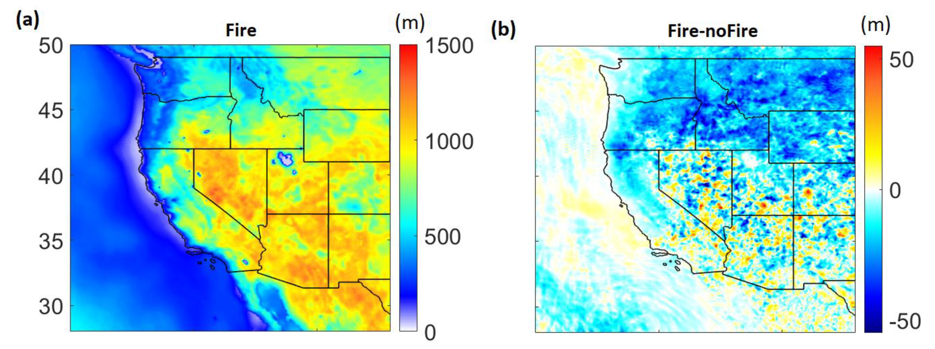
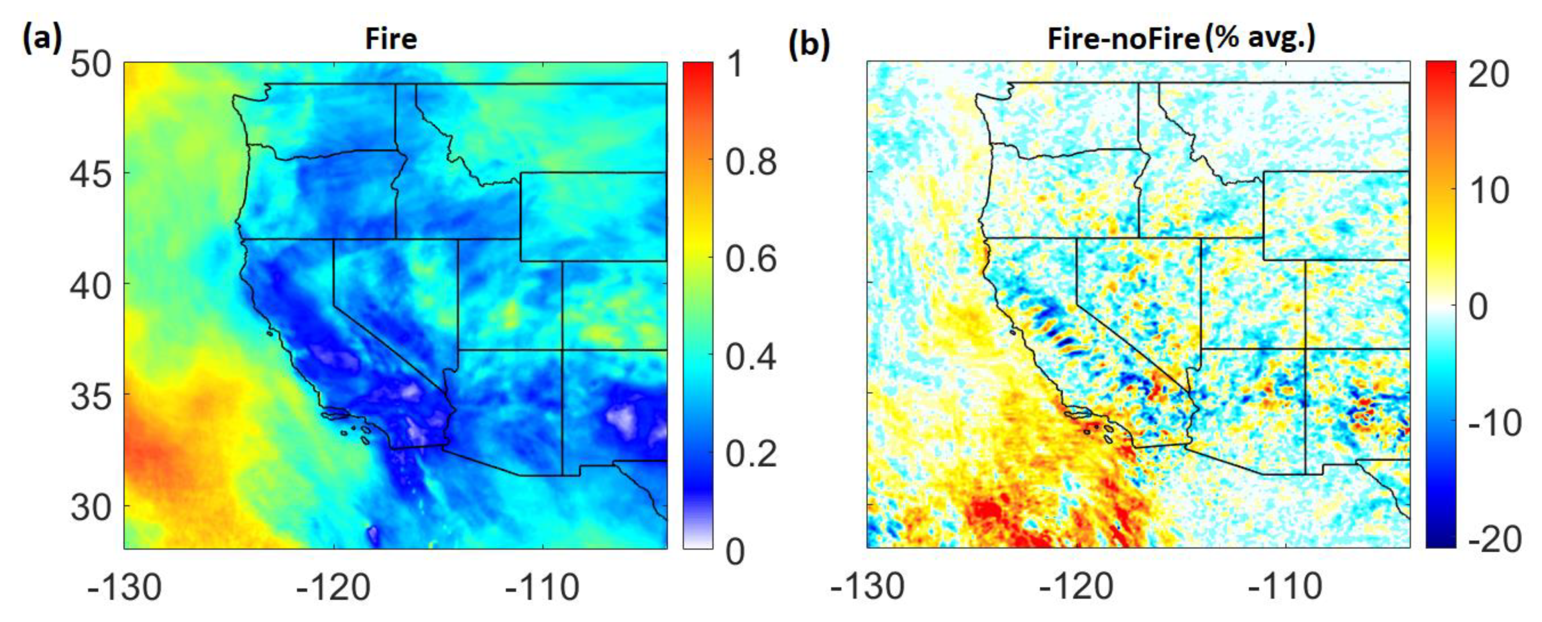
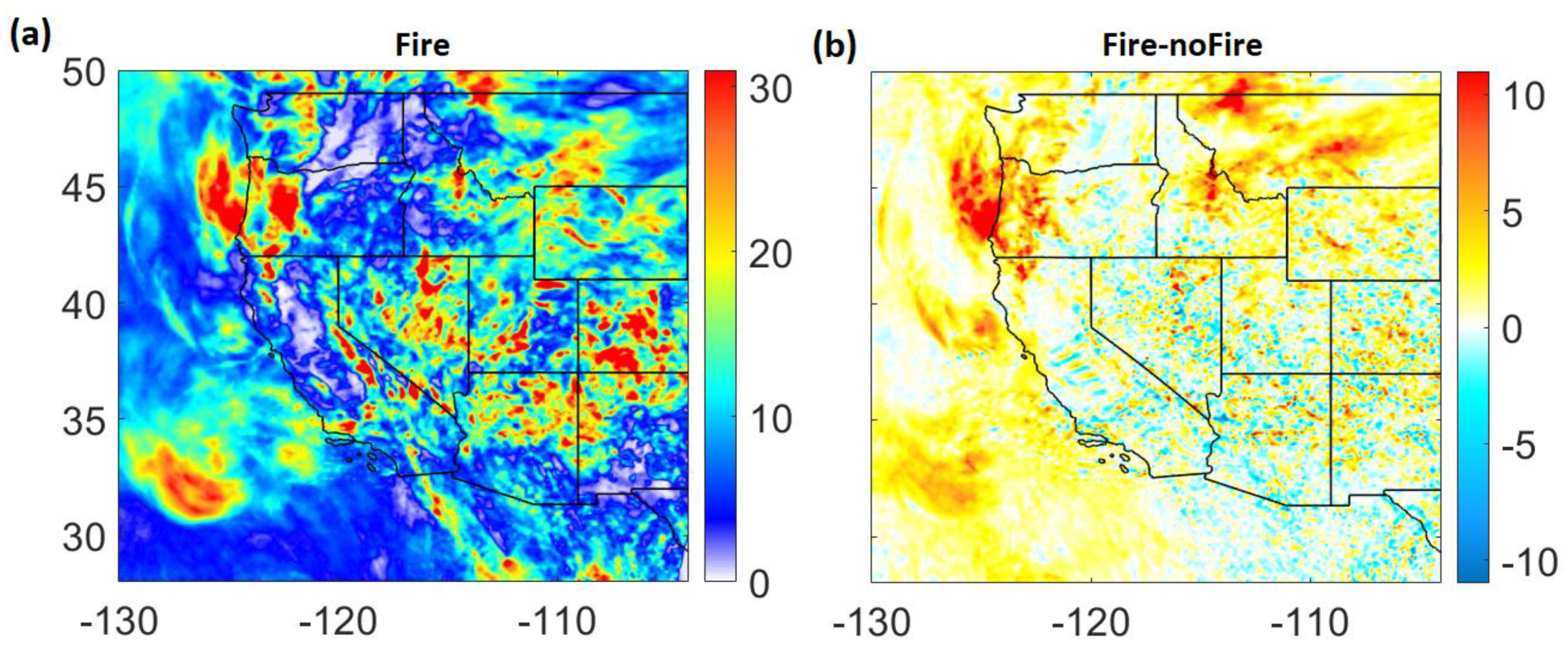
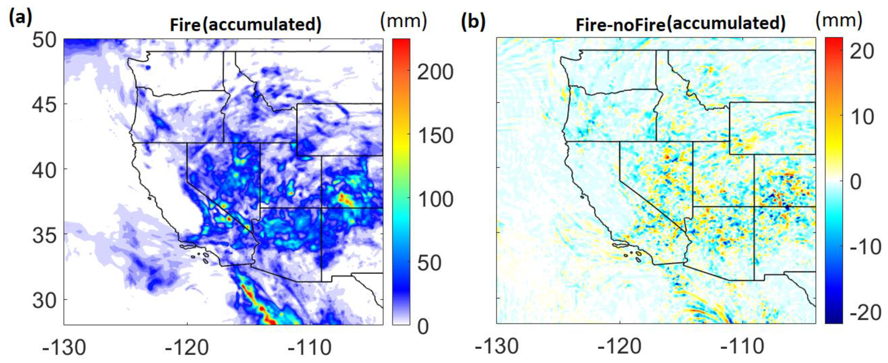
3.2.2. Impact on Clouds, Droplet Number Concentration and Precipitation

Aerosols generated from wildfires are known to impact cloud cover and cloud properties [35,66,67]. Figure 10 shows the changes in cloud cover over the western US due to wildfires. The average cloud cover from the ‘Fire’ simulation is shown in Figure 10a. The difference between the ‘Fire’ and ‘noFire’ simulations, shown in Figure 10b, reveals relatively higher changes in the southern regions including over the ocean. The changes in cloud cover even exceed 20% in some locations (e.g., over south-west marine region). Next, we show changes in cloud optical depth (COD) due to wildfires in Figure 11. The average COD from the ‘Fire’ simulation is shown in Figure 11a along with differences between the ‘Fire’ and ‘noFire’ simulations in Figure 11b. The differences reveal mostly positive changes over Montana, central and eastern Idaho, western Washington and Oregon and over the ocean region. The differences are up to 10 units in some areas of these regions. These changes occur mostly in response to aerosol–cloud interactions in which the aerosol particles act as cloud condensation nuclei to form cloud droplets. Interestingly, the impact of wildfires on COD is quite noticeable in these regions in the north as opposed to cloud cover, which does not change much there. On the other hand, the changes in COD in south regions are mixed with enhancements seen in several locations and reductions seen in the others. Such a mixed response of change in cloud cover and COD in south regions are responsible for similar changes observed for other meteorological variables like near-surface (2 m) temperature and PBLH as discussed earlier.
To analyze aerosol–cloud interaction further, we also look at vertically integrated droplet number concentration and cloud water in Figure 12. Figure 12a shows the droplet number concentration from the ‘Fire’ simulation. There is a strong spatial heterogeneity observed, with the number concentration even exceeding 2 × 10¹⁰ number/m2 in several locations in the domain. The difference between the ‘Fire’ and ‘noFire’ simulation (Figure 12b) reveals mostly enhancements in the northern regions and over the ocean. The enhancements in some locations close to wildfires are more than 1 × 10¹⁰ number/m2 (>200%). Figure 12c shows the spatial distribution of cloud water in the vertical column. Cloud water is high (>25 g m−2) in some regions that also exhibit a high droplet number concentration. The changes in cloud water resulting from wildfires reveal enhancements over western Washington and Oregon, most of the Montana state and over the ocean (Figure 12d). The enhancement is up to 10 g m−2 in some of these locations. The areas showing an increased droplet number concentration accompanied with increased cloud water also exhibit increased cloud optical depth (seen in Figure 11). Some regions (especially in the south) also reveal competing effects of droplet number concentrations and cloud water thus contributing to mixed changes in COD in these regions.
Next, we analyze the impact of wildfires on accumulated precipitation in Figure 13. The precipitation from the ‘Fire’ simulation is more pronounced in the southern regions (Figure 13a) with some locations even receiving precipitation in excess of 200 mm (e.g., in south Colorado). The difference between the ‘Fire’ and ‘noFire’ simulations reveals modification in the spatial distribution of rain in southern regions with accumulated precipitation changing by up to 20 mm in several locations (Figure 13b). The results so far indicate that the impacts of wildfires are not localized but can extend to far regions in form of altered radiation, meteorology, cloud properties and/or precipitation.

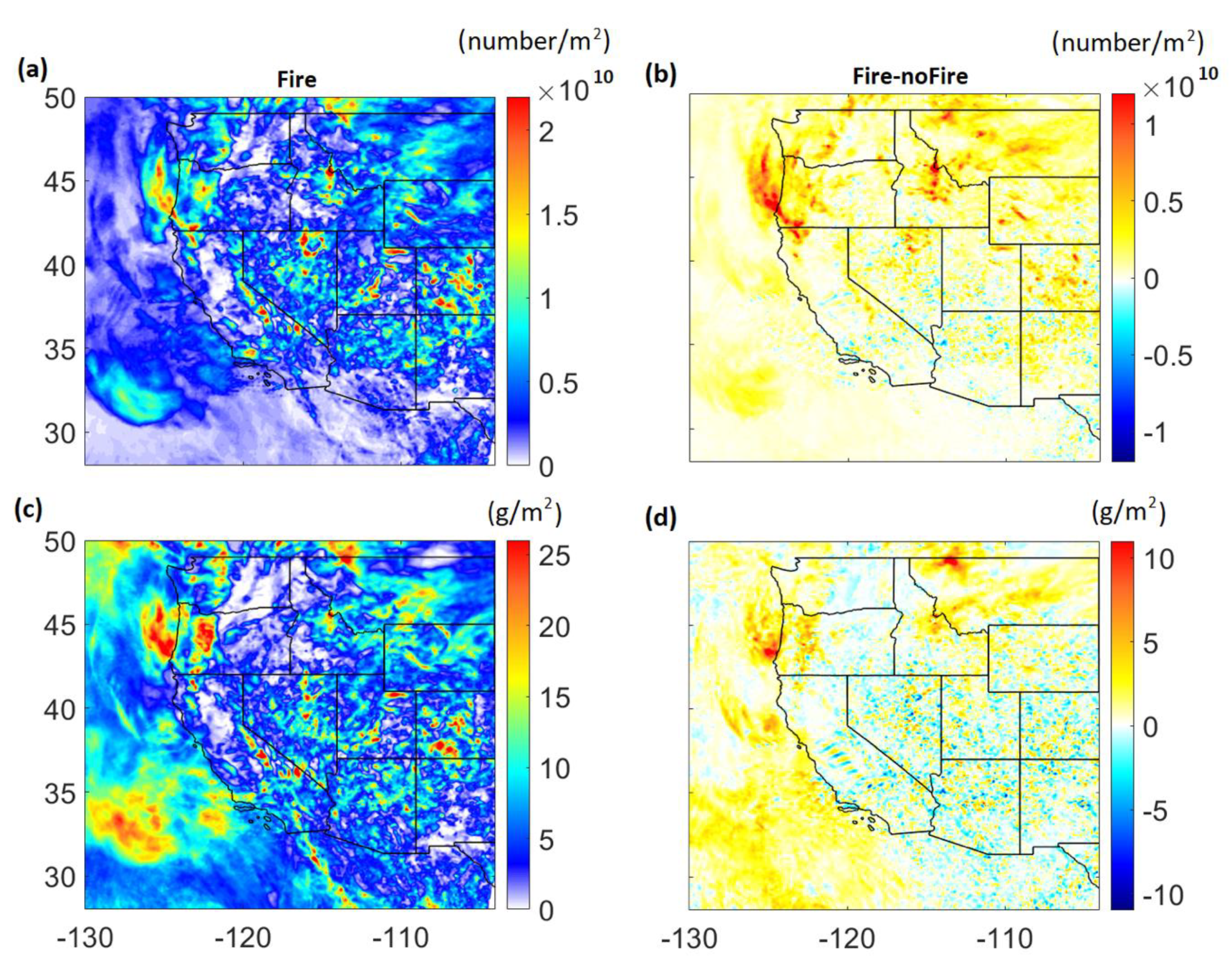
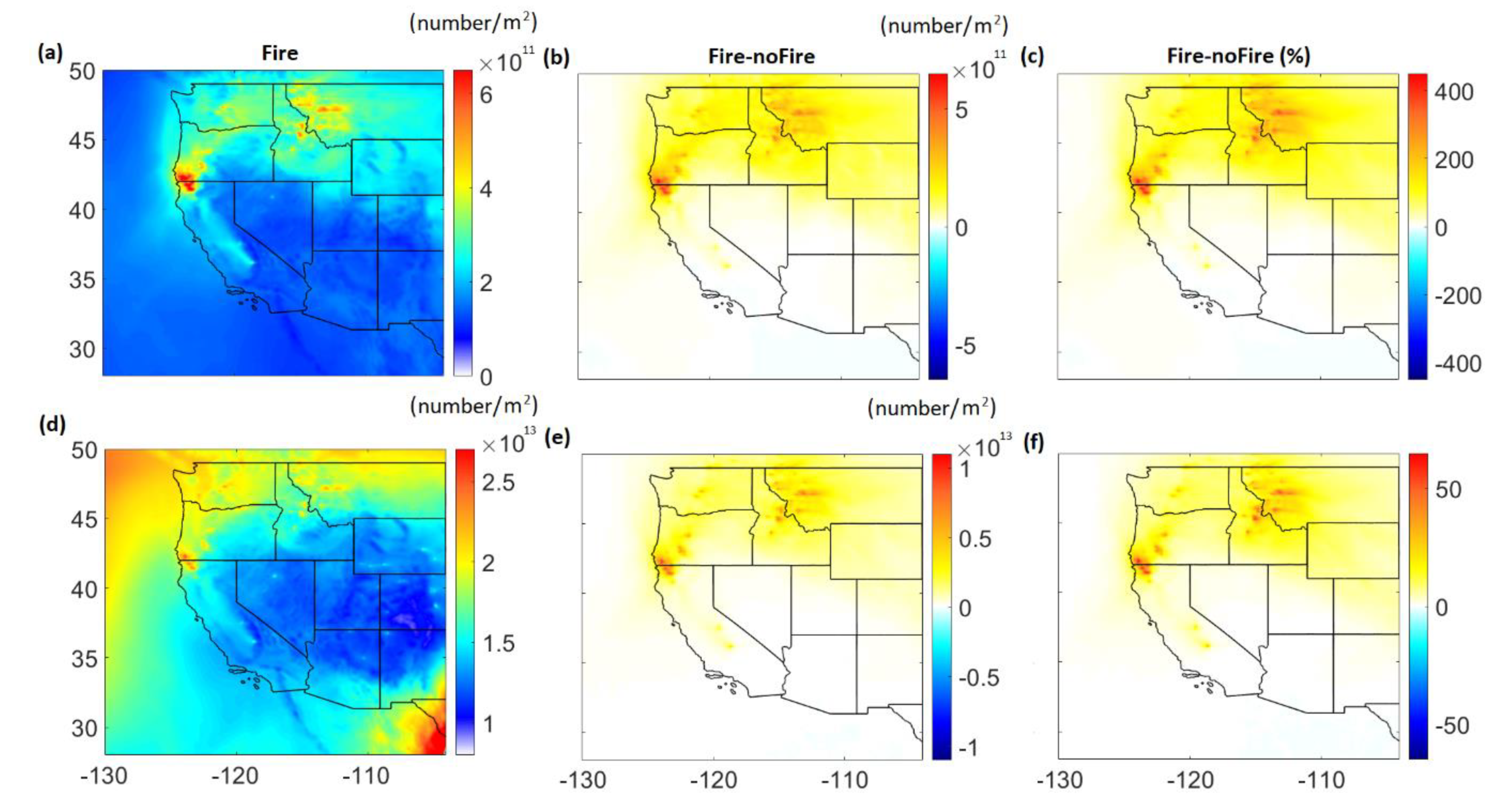
3.2.3. Impact on Cloud Condensation Nuclei (CCN) Activity

We now analyze the sensitivity of potential CCN concentration to supersaturated humidity levels (at supersaturation, S = 0.05% and 0.5%) and wildfire activity. The critical dry diameter for activation is not available from our WRF-Chem output, so we estimated the dry diameter at 0.05% and 0.5% supersaturation, using the equations in Petters et al. [68]. For simplicity, we assume hygroscopicity parameter ( κ ) value of 0.3 for all types of aerosols (background, anthropogenic and wildfires). Based on this, we get dry diameter values of ~262 nm and 57 nm at supersaturation levels of 0.05% and 0.5 %, respectively.
Figure 14a shows the vertically integrated CCN concentration at S = 0.05% (CCN0.05 in number/m2) from the ‘Fire’ simulation. High CCN0.05 concentration (>3 × 10¹¹ number/m2) is seen in areas with intense wildfire activity. The differences between ‘Fire’ and ‘noFire’ simulations (Figure 14b,c) show clear enhancements in CCN0.05 concentration in the northern regions. The differences exceed 5 × 10¹¹ number/m2 (>400%) in some locations close to wildfires. Similarly, Figure 14d shows vertically integrated CCN concentration at S = 0.5% (CCN0.5 in number/m2) from the ‘Fire’ simulation. There is a clear increase in CCN activity at higher supersaturation throughout the domain. High CCN0.5 concentration (>2 × 10¹³ number/m2) is seen not just at wildfire locations but also in remote regions over the ocean. The difference between the ‘Fire’ and ‘noFire’ simulations (Figure 14e) reveals qualitatively similar but quantitatively enhanced absolute changes (by about an order of magnitude more) compared to CCN0.05 (as seen in Figure 14b). The differences are mostly seen over northern US regions with increased CCN0.5 concentration (>1 × 10¹³ number/m2) over wildfire locations (Figure 14e). Contrary to the absolute changes, the percentage changes in CCN0.5 (Figure 14f) between the ‘Fire’ and ‘noFire’ simulations with respect to the ‘noFire’ simulation are smaller (<60%) compared to percentage changes in CCN0.05 (Figure 14c), possibly suggesting an already significant CCN activity in the ‘noFire’ simulation at higher supersaturation.
The percentage changes in CCN concentration at two supersaturation levels potentially reveals some information on the relative size distribution of wildfire aerosol particles with respect to anthropogenic/background aerosol particles. Greater percentage changes in CCN concentration at lower supersaturation, S = 0.05% suggest a high proportion of relatively coarse particles (size > 262 nm) originating from wildfires which can activate into CCN compared to anthropogenic/background aerosol particles. Comparatively, the lower percentage changes in CCN concentration at higher supersaturation, S = 0.5% suggest a high proportion of fine anthropogenic/background aerosol particles in the size range of 57–262 nm which can activate into CCN compared to wildfire aerosol particles.

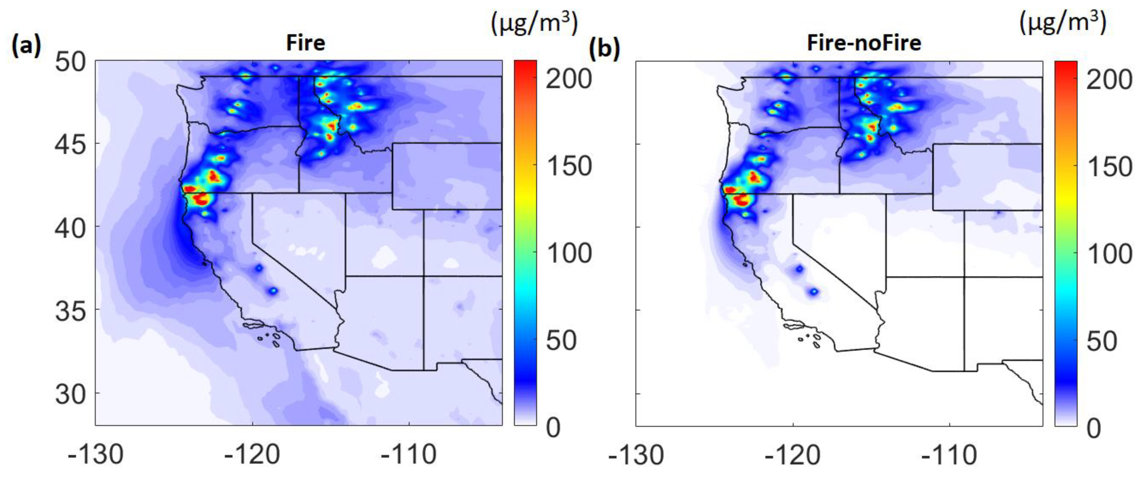
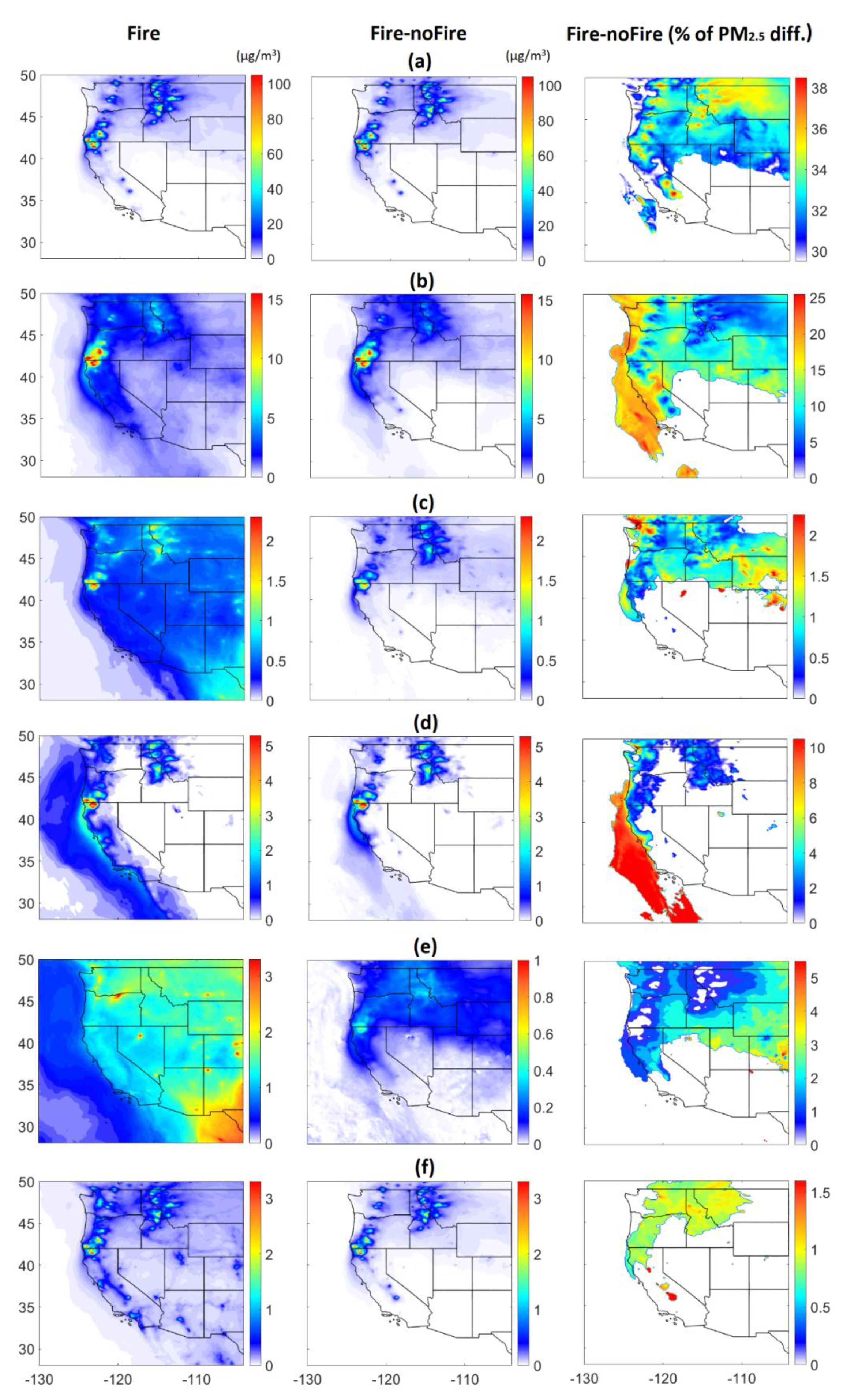
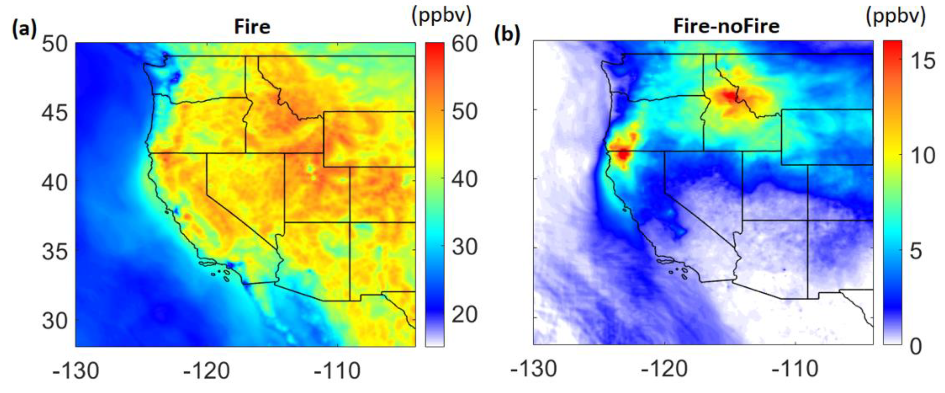
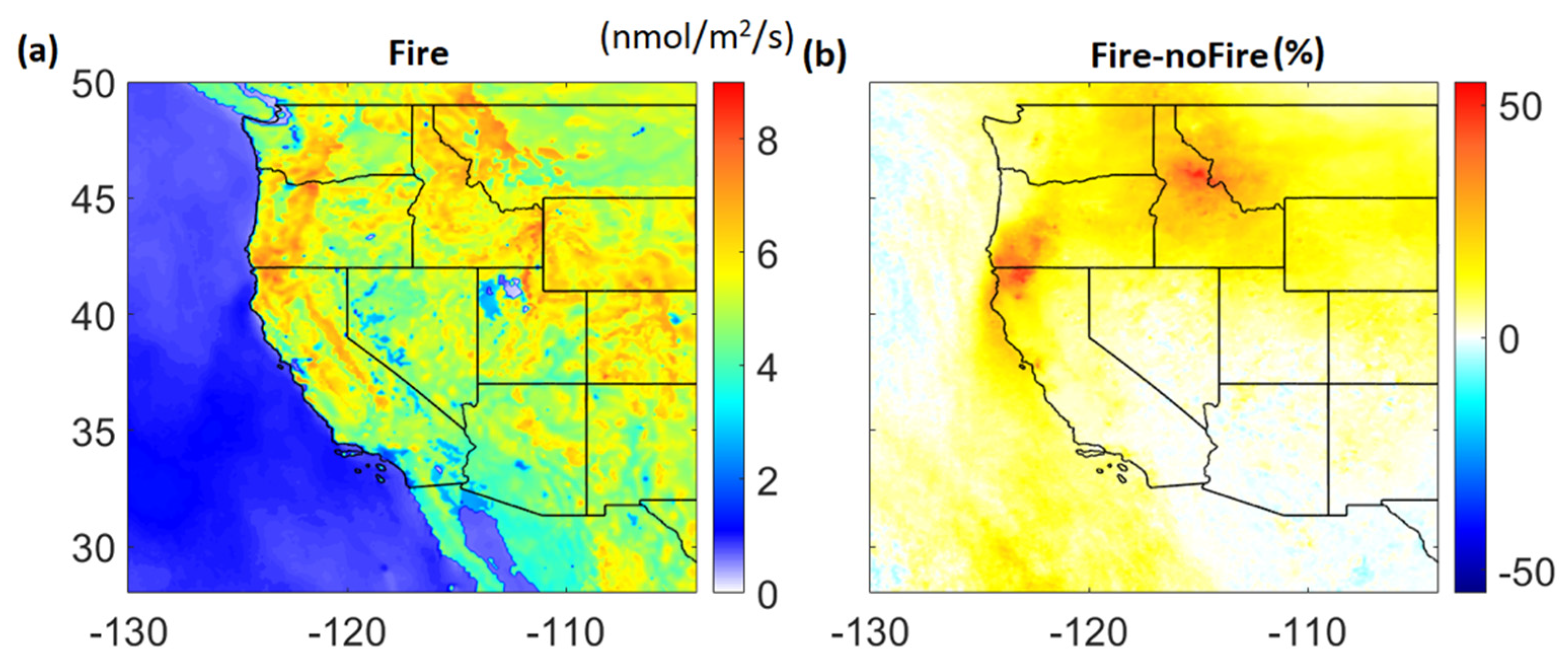
3.2.4. Impact on Air Quality: PM2.5 and Ozone

Next, we analyze the impact of wildfires on air quality. Figure 15 shows the average surface PM2.5 concentrations from the ‘Fire’ simulation (Figure 15a) and the difference between the ‘Fire’ and ‘noFire’ simulations (Figure 15b). As expected, surface PM2.5 levels increase primarily in northern regions. Large changes (even >200 µg m−3) are seen in areas close to wildfires. These enhancements occur not just due to wildfire emissions directly but also in response to changes in meteorology (e.g., suppression of PBLH).
We also show changes in the concentration of surface PM2.5 chemical components in Figure 16. The changes are high for primary organic carbon (POC) concentrations with differences even exceeding 100 µg m−3 in locations close to wildfire activity (Figure 16a). The POC changes in the vicinity of the wildfires contribute to about 35% or more of the PM2.5 enhancements due to wildfires (Figure 16a; rightmost column). In the rest of the northern regions also (except some areas in western Washington and Oregon), POC contributes to more than 30% of PM2.5 enhancement due to wildfires. Secondary organic aerosols (SOA) contribute to more than 15 µg m−3 of PM2.5 changes in locations close to wildfires in south Oregon and north California (Figure 16b; middle column). The contribution of SOA differences to PM2.5 changes in wildfire locations is mostly less than 10% (Figure 16b; rightmost column). The contribution of SOA to PM2.5 enhancement increases away from wildfires although the absolute changes in SOA reduce (Figure 16b) as seen for other chemical species and total PM2.5. The contribution of species like Ammonium (NH4+), Nitrate (NO3), Sulfate (SO42−) and Black Carbon (BC) to PM2.5 enhancements over land regions is generally less than 5% each. The remaining increase in surface PM2.5 levels due to wildfires is due to changes in the concentration of other inorganics (mineral dust) (not shown).
Next, we show the changes in surface ozone mixing ratios due to wildfires in Figure 17. The average mixing ratio during this period is more than 35 ppbv over most of the western US (Figure 17a). The surface mixing ratios increase due to wildfires in the entire north and some south regions (Figure 17b). The enhancements are up to 15 ppbv in areas close to wildfires. Again, these enhancements are not just attributed to wildfire emissions but also the feedback of these emissions on meteorology (e.g., suppressed PBLH potentially causing an increase in ozone precursor concentrations). Considering the importance of the dry deposition process as an important sink for tropospheric ozone [69,70,71,72], we also analyze the contribution of dry deposition processes to surface ozone levels in Figure 18. The average dry deposition flux from the ‘Fire’ run (Figure 18a) is greater than 4 nmol m−2 s−1 over most of the western US whereas it is mostly under 2 nmol m−2 s−1 over ocean regions. The flux increases due to wildfires over the north regions (Figure 18b) and over some areas in the south including over the ocean. The flux enhancements are higher by 50% in locations close to wildfires. Such enhancements in ozone dry deposition flux to the terrestrial surface might be significant in modulating the surface ozone mixing ratios during wildfire episodes, although it can potentially cause damage to the vegetation and reduction in agricultural productivity [73,74,75,76,77].

4. Conclusions

In this study, we analyze the impact of wildfire emissions on meteorology and air quality over the western US while considering the aerosol–cloud–radiation interactions in meteorology–chemistry coupled with the WRF-Chem model for wildfire episodes in September 2017. WRF-Chem performed reasonably well when evaluated against AQS measurements (2 m temperature, 10 m wind speed, surface PM2.5 concentrations and surface ozone mixing ratios). The model shows good performance for 2 m temperature with results at 89% AQS locations within recommended performance criteria (corresponding to mean bias value within ±1 K together with gross error value < 3 K) and 98% of locations showing a correlation coefficient (r) value greater than 0.7. For 10 m wind speed, the model’s performance is reasonable with 67% locations within the recommended performance criteria (corresponding to mean bias value within ±0.5 m s−1 together with RMSE value < 2 m s−1) and 77% of locations having an r value greater than 0.5. Weak model performance for wind speed at several locations could be due to coarse model resolution (12 km × 12 km) which might not be enough to adequately resolve topography. For PM2.5, the model shows a moderate performance with 86% of locations within the recommended performance criteria (corresponding to normalized mean error values within 0–75% together with normalized mean bias values within ±60%) and 62% of locations having an r value greater than 0.5. The model exhibits a high positive bias for PM2.5 (MB ≥ 5 μg m−3; NMB ≥ 15%) at some stations in the vicinity of the wildfires (e.g., western Washington) while compensating at other stations in the vicinity of the wildfires (e.g., eastern Washington) by underestimating PM2.5 indicating possible uncertainty in wildfire emissions and the vertical plume distribution in the model. The model also overestimates PM2.5 in some coastal locations in California (though MB is within ±5 μg m−3) and a few stations inland. At the remaining stations, the model tends to underpredict the PM2.5 concentrations, which could be associated with wildfire and anthropogenic emissions (e.g., uncertainties in emissions and the fact that the NEI inventory used in this study is representative of the year 2014). Finally, the model performs reasonably well for surface ozone with 98% of locations within the recommended performance criteria and 95% of locations having an r value greater than 0.5. The model’s mean bias for ozone is within ±30% at most of the stations.
The model also performs well when evaluated against MODIS satellite data (shortwave surface downward radiation, outgoing longwave radiation, cloud fraction and cloud optical depth). The spatial correlation coefficient between the model and MODIS for shortwave surface downward radiation (SSDR) is 0.92 with a mean bias of −0.65 W m−2 (NMB of ~−0.3%) and 0.96 for outgoing longwave radiation with a mean bias of 4.7 W m−2 (NMB of ~1.8%). Similarly, the spatial correlation coefficient between the model and MODIS for cloud fraction is 0.70 with a mean bias of −0.10 (~−18%) over the domain. The model’s underprediction is primarily attributed to the underprediction of cloud cover over the ocean region. The model performs reasonably well for cloud optical depth in north and eastern regions but tends to underpredict in other areas (south-west) over the western US. This is possibly due to missing satellite data for cloud optical depth in some regions on several days for the analysis period as seen in daily satellite outputs. Nevertheless, considering the model’s acceptable performance for other variables and its ability to capture cloud cover we further examine the impact of wildfires on meteorology and air quality for the first half of September 2017 when fire activity was relatively intense.
The model showed a reduction in daytime shortwave downward radiation in the north and over the coastal regions due to aerosol–cloud–radiation interaction. The average reduction in some locations close to wildfires is up to 50 W m−2. This results in the reduction of average surface temperature (by up to 0.5 °C) in the northern regions. In the south, the effects are mixed with some locations even experiencing a warming effect on average, which is mostly attributed to rapid changes in cloud cover/cloud optical depth, resulting in cloud radiative effects. The cooling near the surface in north regions led to reduced atmospheric turbulence and hence resulted in suppressed planetary boundary layer height (PBLH) by up to 50 m in some locations. The reductions in PBLH can lead to reduced vertical mixing of the pollutants (PM2.5 and O3 precursors), thus leading to further enhancements of the pollutant concentrations near the surface in addition to a direct contribution from the wildfires.
The model shows changes in cloud cover by more than 20% in some locations in the south domain including over the ocean. Furthermore, the model reveals quite noticeable and mostly positive changes in cloud optical depth (COD) in several areas in the north. The changes exceed 10 units in some areas in these regions. These changes occur mostly in response to aerosol–cloud interactions. Further analyses of results for aerosol–cloud interactions reveal enhancements in vertically integrated droplet number concentration (by greater than 200%) and cloud water (by upto 10 g m−2) in locations showing positive changes in COD. Some regions (especially in the south) also reveal competing effects of droplet number concentration and cloud water thus contributing to mixed changes in COD in these regions. The model also showed modification in the spatial distribution of rain in southern regions with accumulated precipitation changing by up to 20 mm in several locations.
We further investigated the sensitivity of potential CCN concentration to supersaturated humidity levels (at supersaturation, S = 0.05% and 0.5%) and wildfire activity. The CCN concentration increases due to wildfires at both supersaturation levels primarily in the northern regions. The enhancement in CCN concentration due to wildfires at lower supersaturation level, S = 0.05%, is found to be more than 400% in some locations close to wildfires. Comparatively, the enhancement in CCN concentration due to wildfires at a higher supersaturation level, S = 0.5%, is found to be up to 60%. In contrast to percentage changes, the absolute changes are higher at higher supersaturation (S = 0.5%) compared to that at lower supersaturation (S = 0.05%) by about an order of magnitude. The contrast between percentage changes and absolute changes at the two supersaturation levels reveals a higher proportion of relatively coarse particles (size > 262 nm) and a lower proportion of fine particles (size range 57–262 nm) originating from wildfires that activate into CCN compared to anthropogenic/background aerosol particles.
Next, we analyze the impact of wildfires on air quality. Large changes in average PM2.5 concentrations (>200 μg m−3) are seen in areas close to wildfires. These enhancements occur not just due to wildfire emissions directly but also in response to changes in meteorology (e.g., suppression of PBLH). A significant proportion of these enhancements in PM2.5 is due to primary organic carbon (>30%) from wildfires. The contribution of secondary organic aerosols to PM2.5 enhancements is less than 10% in wildfire locations species like ammonium, nitrate, sulphate and black carbon, which contribute less than 5% each to PM2.5 enhancements over land regions. The remaining increase in surface PM2.5 levels due to wildfires is due to changes in concentration of other inorganics (mineral dust). Surface ozone mixing ratios increase due to wildfires in the entire north and some south regions with enhancements up to 15 ppbv in areas close to wildfires. Again, these changes are not just attributed to wildfire emissions but also the feedback of these emissions on meteorology (e.g., suppressed PBLH potentially causing an increase in precursor concentrations).
The results in this study are applicable to only September 2017 wildfires over the western US but may present a general idea of the impacts that the wildfires can have in this part of the world. The model setup in the study is beneficial for the modeling community for other applications related to meteorology and/or air quality over this region (e.g., assessing air quality-related health impacts of wildfire emissions). Such a model setup can also be used to examine the future impacts of wildfires by making use of future wildfire projections [13]. The limitations in this study arise from several factors like uncertainties in fire emissions [52,78] and computational costs associated with conducting simulations at further high resolution (<12 km spatial resolution) in order to resolve topography to a greater degree. Moreover, a study by Carter et al. [79] revealed large differences between various fire emission inventories, with the FINN inventory underestimating fires over North America. Such underestimation of fires in the FINN inventory would possibly lead to conservative estimates in our study. Nevertheless, the results in this study show that the impacts of wildfires are not localized but can extend to far regions in the form of altered radiation, meteorology, cloud properties and/or precipitation and change in air quality. Such impacts (although possibly short-lived) are likely to intensify with an increase in wildfire intensity and duration in the future [13], thus calling for possible adaptation strategies.

Author Contributions

Conceptualization, Y.L.; Formal analysis, A.S.; Funding acquisition, Y.L.; Resources, Y.L.; Software, Y.L., A.S. and A.C.F.V.; Supervision, Y.L.; Validation, A.S.; Writing—original draft, A.S.; Writing—review & editing, A.S., A.C.F.V. and Y.L. All authors have read and agreed to the published version of the manuscript.

Funding

The authors acknowledge partial funding by the Washington State Department of Ecology.

Institutional Review Board Statement

Not applicable.

Informed Consent Statement

Not applicable.

Data Availability Statement

Global Forecast System (GFS) analysis dataset is available at www.ncdc.noaa.gov/data-access/model-data/model-datasets/global-forcast-system-gfs; last accessed on 31 January 2022. The preprocessors and inputs for biogenic and biomass-burning emissions are available at NCAR Atmospheric Chemistry Observations and Modeling website (www.acom.ucar.edu/wrf-chem/download.shtml; last accessed on 31 January 2022). NEI 2014 emission data are available at https://www2.acom.ucar.edu/wrf-chem/wrf-chem-tools-community; last accessed on 31 January 2022. MOZART-4/GEOS5 output to prepare chemical initial and boundary conditions is available at https://www.acom.ucar.edu/wrf-chem/mozart.shtml; last accessed on 31 January 2022. Surface measurements from the U.S. Environmental Protection Agency (EPA) Air Quality System (AQS) is available at https://www.epa.gov/aqs, last accessed on 31 January 2022.

Acknowledgments

Model simulations were performed on the Kamiak HPC (https://hpc.wsu.edu/; last accessed on 31 January 2022) at Washington State University, Pullman campus (Pullman, Washington, USA). We acknowledge Alison Eyth and Barron H. Henderson at the U.S. Environmental Protection Agency (EPA, Washington, DC, USA) for making SMOKE outputs available and to Gabriele Pfister and Stacy Walters at the National Center for Atmospheric Research (NCAR, Boulder, CO, USA) and Stu McKeen at the National Oceanic and Atmospheric Administration (NOAA, Washington, DC, USA) for developing and providing tools to integrate SMOKE emissions into WRF-Chem.

Conflicts of Interest

The authors declare that they have no conflict of interest.

References

  1. DeBell, L.J.; Talbot, R.W.; Dibb, J.E.; Munger, J.W.; Fischer, E.V.; Frolking, S.E. A major regional air pollution event in the northeastern United States caused by extensive forest fires in Quebec, Canada. J. Geophys. Res.-Atmos. 2004, 109, D19305. [Google Scholar] [CrossRef] [Green Version]
  2. McMeeking, G.R.; Kreidenweis, S.M.; Lunden, M.; Carrillo, J.; Carrico, C.M.; Lee, T.; Herckes, P.; Engling, G.; Day, D.E.; Hand, J.; et al. Smoke-impacted regional haze in California during the summer of 2002. Agric. For. Meteorol. 2006, 137, 25–42. [Google Scholar] [CrossRef]
  3. Val Martin, M.; Honrath, R.; Owen, R.; Pfister, G.; Fialho, P.; Barate, F. Significant enhancements of nitrogen oxides, black carbon, and ozone in the North Atlantic lower free troposphere resulting from North American boreal wildfires. J. Geophys. Res. 2006, 111, D23S60. [Google Scholar] [CrossRef] [Green Version]
  4. Pfister, G.G.; Wiedinmyer, C.; Emmons, L.K. Impacts of the fall 2007 California wildfires on surface ozone: Integrating local observations with global model simulations. Geophys. Res. Lett. 2008, 35, L19814. [Google Scholar] [CrossRef] [Green Version]
  5. Archer-Nicholls, S.; Lowe, D.; Schultz, D.M.; McFiggans, G. Aerosol–radiation–cloud interactions in a regional coupled model: The effects of convective parameterisation and resolution. Atmos. Chem. Phys. 2016, 16, 5573–5594. [Google Scholar] [CrossRef] [Green Version]
  6. Charlson, R.J.; Schwartz, S.E.; Hales, J.M.; Cess, R.D.; Coakley, J.A., Jr.; Hansen, J.E.; Hofmann, D.J. Climate Forcing by Anthropogenic Aerosols. Science 1992, 255, 423–430. [Google Scholar] [CrossRef]
  7. Chand, D.; Wood, R.; Anderson, T.L.; Satheesh, S.K.; Charlson, R.J. Satellite-derived direct radiative effect of aerosols dependent on cloud cover. Nat. Geosci. 2009, 2, 181–184. [Google Scholar] [CrossRef]
  8. Haywood, J.; Boucher, O. Estimates of the direct and indirect radiative forcing due to tropospheric aerosols: A review. Rev. Geophys. Geophys. 2000, 38, 513. [Google Scholar] [CrossRef]
  9. Zhang, Y.; Fu, R.; Yu, H.; Dickinson, R.E.; Juarez, R.N.; Chin, M.; Wang, H. A regional climate model study of how biomass burning aerosol impacts land–atmosphere interactions over the Amazon. J. Geophys. Res. 2008, 113, D14S15. [Google Scholar] [CrossRef] [Green Version]
  10. Westerling, A.; Hidalgo, H.; Cayan, D.; Swetnam, T. Warming and earlier spring increases western U.S. forest wildfire activity. Science 2006, 313, 940–943. [Google Scholar] [CrossRef] [Green Version]
  11. Holden, Z.A.; Swanson, A.; Luce, C.H.; Jolly, W.M.; Maneta, M.; Oyler, J.W.; Warren, D.A.; Parsons, R.; Affleck, D. Decreasing fire season precipitation increased recent western US forest wildfire activity. Proc. Natl. Acad. Sci. USA 2018, 115, E8349–E8357. [Google Scholar] [CrossRef] [PubMed] [Green Version]
  12. Knapp, A.P.; Soule, T.P. Spatio-temporal linkages between declining Arctic sea-ice extent and increasing wildfire activity in the western United States. Forests 2017, 8, 313. [Google Scholar] [CrossRef] [Green Version]
  13. Spracklen, D.V.; Mickley, L.J.; Logan, J.A.; Hudman, R.C.; Yevich, R.; Flannigan, M.D.; Westerling, A.L. Impacts of climate change from 2000 to 2050 on wildfire activity and carbonaceous aerosol concentrations in the western United States. J. Geophys. Res. 2009, 114, D20301. [Google Scholar] [CrossRef]
  14. Mallia, D.V.; Lin, J.C.; Urbanski, S.; Ehleringer, J.; Nehrkorn, T. Impacts of upwind wildfire emissions on CO, CO2, and PM2.5 concentrations in Salt Lake City, Utah. J. Geophys. Res. Atmos. 2015, 120, 147–166. [Google Scholar] [CrossRef]
  15. Lu, X.; Zhang, L.; Yue, X.; Zhang, J.; Jaffe, D.A.; Stohl, A.; Zhao, Y.; Shao, J. Wildfire influences on the variability and trend of summer surface ozone in the mountainous western United States. Atmos. Chem. Phys. 2016, 16, 14687–14702. [Google Scholar] [CrossRef] [Green Version]
  16. McClure, C.D.; Jaffe, D.A. Investigation of high ozone events due to wildfire smoke in an urban area. Atmos. Environ. 2018, 194, 146–157. [Google Scholar] [CrossRef]
  17. Wilkins, J.L.; George, P.; Kristen, F.; Wyat, A.; Pierce, T. The impact of US wildland fires on ozone and particulate matter: A comparison of measurements and CMAQ model predictions from 2008 to 2012. Int. J. Wildl. Fire 2018, 27, 684–698. [Google Scholar] [CrossRef]
  18. Buysse, C.E.; Kaulfus, A.; Nair, U.; Jaffe, D.A. Relationships between particulate matter, ozone, and nitrogen oxides during urban smoke events in the western US. Environ. Sci. Technol. 2019, 53, 12519–12528. [Google Scholar] [CrossRef]
  19. O’Dell, K.; Ford, B.; Fischer, E.V.; Pierce, J.R. Contribution of wildland-fire smoke to US PM2.5 and its influence on recent trends. Environ. Sci. Technol. 2019, 53, 1797–1804. [Google Scholar] [CrossRef]
  20. Xie, Y.; Lin, M.; Horowitz, L.W. Summer PM2.5 pollution extremes caused by wildfires over the western United States during 2017–2018. Geophys. Res. Lett. 2020, 47, e2020GL089429. [Google Scholar] [CrossRef]
  21. Zhang, A.; Liu, Y.; Goodrick, S.; Williams, M.D. Duff burning from wildfires in a moist region: Different impacts on PM2.5 and ozone. Atmos. Chem. Phys. 2022, 22, 597–624. [Google Scholar] [CrossRef]
  22. Delfino, R.J.; Brummel, S.; Wu, J.; Stern, H.; Ostro, B.; Lipsett, M.; Winer, A.; Street, D.H.; Zhang, L.; Tjoa, T.; et al. The relationship of respiratory and cardiovascular hospital admissions to the southern California wildfires of 2003. Occup. Environ. Med. 2009, 66, 189–197. [Google Scholar] [CrossRef] [PubMed] [Green Version]
  23. Rappold, A.G.; Stone, S.L.; Cascio, W.E.; Neas, L.M.; Kilaru, V.J.; Carraway, M.S.; Szykman, J.J.; Ising, A.; Cleve, W.E.; Meredith, J.T.; et al. Peat bog wildfire smoke exposure in rural North Carolina is associated with cardiopulmonary emergency department visits assessed through syndromic surveillance. Environ. Health Perspect. 2011, 119, 1415–1420. [Google Scholar] [CrossRef] [Green Version]
  24. Henderson, S.B.; Brauer, M.; Macnab, Y.C.; Kennedy, S.M. Three measures of forest fire smoke exposure and their associations with respiratory and cardiovascular health outcomes in a population-based cohort. Environ. Health Perspect. 2011, 119, 1266–1271. [Google Scholar] [CrossRef]
  25. Reid, C.E.; Considine, E.M.; Watson, G.L.; Telesca, D.; Pfister, G.G.; Jerrett, M. Associations between respiratory health and ozone and fine particulate matter during a wildfire event. Environ. Int. 2019, 129, 291–298. [Google Scholar] [CrossRef]
  26. Doubleday, A.; Schulte, J.; Sheppard, L.; Kadlec, M.; Dhammapala, R.; Fox, J.; Isaksen, T.B. Mortality associated with wildfire smoke exposure in Washington state, 2006–2017: A case-crossover study. Environ. Health 2020, 19, 4. [Google Scholar] [CrossRef] [Green Version]
  27. Ford, B.; Val Martin, M.; Zelasky, S.E.; Fischer, E.V.; Anenberg, S.C.; Heald, C.L.; Pierce, J.R. Future fire impacts on smoke concentrations, visibility, and health in the contiguous United States. GeoHealth 2018, 2, 229–247. [Google Scholar] [CrossRef] [PubMed] [Green Version]
  28. Jiang, X.; Wiedinmyer, C.; Carlton, A.G. Aerosols from fires: An examination of the effects on ozone photochemistry in the Western United States. Environ. Sci. Technol. 2012, 46, 11878–11886. [Google Scholar] [CrossRef]
  29. Grell, G.A.; Peckham, S.E.; McKeen, S.; Schmitz, R.; Frost, G.; Skamarock, W.C.; Eder, B. Fully coupled “online” chemistry within the WRF model. Atmos. Environ. 2005, 39, 6957–6975. [Google Scholar] [CrossRef]
  30. Fast, J.D.; Gustafson, W.I., Jr.; Easter, R.C.; Zaveri, R.A.; Barnard, J.C.; Chapman, E.G.; Grell, G.A.; Peckham, S.E. Evolution of ozone, particulates, and aerosol direct radiative forcing in the vicinity of Houston using a fully-coupled meteorology-chemistry aerosol model. J. Geophys. Res. 2006, 111, D21305. [Google Scholar] [CrossRef]
  31. McKeen, S.; Wilczak, J.; Grell, G.; Djalalova, I.; Peckham, S.; Hsie, E.-Y.; Gong, W.; Bouchet, V.; Menard, S.; Moffet, R.; et al. Assessment of an ensemble of seven real-time ozone forecasts over Eastern North America during the summer of 2004. J. Geophys. Res. 2005, 110, D21307. [Google Scholar] [CrossRef]
  32. Kumar, R.; Naja, M.; Pfister, G.G.; Barth, M.C.; Brasseur, G.P. Simulations over South Asia using the Weather Research and Forecasting model with Chemistry (WRF-Chem): Set-up and meteorological evaluation. Geosci. Model Dev. 2012, 5, 321–343. [Google Scholar] [CrossRef] [Green Version]
  33. Powers, J.G.; Klemp, J.B.; Skamarock, W.C.; Davis, C.A.; Dudhia, J.; Gill, D.O.; Coen, J.L.; Gochis, D.J.; Ahmadov, R.; Peckham, S.E.; et al. The weather research and forecasting model: Overview, system efforts, and future directions. B. Am. Meteorol. Soc. 2017, 98, 1717–1737. [Google Scholar] [CrossRef]
  34. Fast, J.; Aiken, A.C.; Allan, J.; Alexander, L.; Campos, T.; Canagaratna, M.R.; Chapman, E.; DeCarlo, P.F.; de Foy, B.; Gaffney, J.; et al. Evaluating simulated primary anthropogenic and biomass burning organic aerosols during MILAGRO: Implications for assessing treatments of secondary organic aerosols. Atmos. Chem. Phys. 2009, 9, 6191–6215. [Google Scholar] [CrossRef] [Green Version]
  35. Grell, G.; Freitas, S.R.; Stuefer, M.; Fast, J. Inclusion of biomass burning in WRF-Chem: Impact of wildfires on weather forecasts. Atmos. Chem. Phys. 2011, 11, 5289–5303. [Google Scholar] [CrossRef] [Green Version]
  36. Broxton, P.D.; Zeng, X.; Sulla-Menashe, D.; Troch, P.A. A global land cover climatology using MODIS data. J. Appl. Meteorol. Climatol. 2014, 53, 1593–1605. [Google Scholar] [CrossRef]
  37. Zhang, N.; Chen, Y.; Gao, H.; Luo, L. Influence of urban land cover data uncertainties on the numerical simulations of urbanization effects in the 2013 high-temperature episode in Eastern China. Theor. Appl. Climatol. 2019, 138, 1715–1734. [Google Scholar] [CrossRef] [Green Version]
  38. Morrison, H.; Curry, J.A.; Khvorostyanov, V.I. A new double- moment microphysics parameterization for application in cloud and climate models. Part I: Description. J. Atmos. Sci. 2005, 62, 1665–1677. [Google Scholar] [CrossRef]
  39. Grell, G.A.; Freitas, S.R. A scale and aerosol aware stochastic convective parameterization for weather and air quality modeling. Atmos. Chem. Phys. 2014, 14, 5233–5250. [Google Scholar] [CrossRef] [Green Version]
  40. Mlawer, E.J.; Taubman, S.J.; Brown, P.D.; Iacono, M.J.; Clough, S.A. Radiative transfer for inhomogeneous atmosphere: RRTM, a validated correlated-k model for the long-wave. J. Geophys. Res. 1997, 102, 16663–16682. [Google Scholar] [CrossRef] [Green Version]
  41. Chou, M.-D.; Suarez, M.J. An Efficient Thermal Infrared Radiation Parameterization for Use in General Circulation Models; NASA Technical Memorandum 104606; NASA, Goddard Space Flight Center: Greenbelt, MD, USA, 1994; Volume 3, p. 85. [Google Scholar]
  42. Tewari, M.; Chen, F.; Wang, W.; Dudhia, J.; Lemone, M.A.; Mitchell, K.E.; Ek, M.; Gayno, G.; Wegiel, J.W.; Cuenca, R. Implementation and verification of the unified Noah land-surface model in the WRF model. In Proceedings of the 20th Conference on Weather Analysis and Forecasting/16th Conference on Numerical Weather Prediction, Seattle, WA, USA, 14 January 2004; pp. 11–15. [Google Scholar]
  43. Monin, A.S.; Obukhov, A.M. Basic laws of turbulent mixing in the surface layer of the atmosphere. Tr. Geofiz. Inst. Akad. Nauk SSSR 1954, 24, 163–187. [Google Scholar]
  44. Janjic, Z.I. The step-mountain eta coordinate model: Further developments of the convection, viscous sublayer and turbulence closure schemes. Mon. Weather Rev. 1994, 122, 927–945. [Google Scholar] [CrossRef] [Green Version]
  45. Janjic, Z.I. The surface layer in the NCEP Eta Model. In Proceedings of the Eleventh Conference on Numerical Weather Prediction, Norfolk, VA, USA, 19–23 August 1996; American Meteorological Society: Boston, MA, USA, 1996; pp. 354–355. [Google Scholar]
  46. Bougeault, P.; LaCarrere, P. Parameterization of orography-induced turbulence in a mesobeta-scale model. Mon. Wea. Rev. 1989, 117, 1872–1890. [Google Scholar] [CrossRef]
  47. Emmons, L.K.; Walters, S.; Hess, P.G.; Lamarque, J.-F.; Pfister, G.G.; Fillmore, D.; Granier, C.; Guenther, A.; Kinnison, D.; Laepple, T.; et al. Description and evaluation of the Model for Ozone and Related chemical Tracers, version 4 (MOZART-4). Geosci. Model Dev. 2010, 3, 43–67. [Google Scholar] [CrossRef] [Green Version]
  48. Zaveri, R.A.; Easter, R.C.; Fast, J.D.; Peters, L.K. Model for simulating aerosol interactions and chemistry (MOSAIC). J. Geophys. Res. 2008, 113, D132024. [Google Scholar] [CrossRef]
  49. Madronich, S. Photodissociation in the atmosphere: 1. Actinic flux and the effect of ground reflections and clouds. J. Geophys. Res. 1987, 92, 9740–9752. [Google Scholar] [CrossRef]
  50. Wesely, M.L. Parameterization of Surface Resistance to Gaseous Dry Deposition in Regional Numerical Models. Atmos. Environ. 1989, 23, 1293–1304. [Google Scholar] [CrossRef]
  51. Guenther, A.; Karl, T.; Harley, P.; Wiedinmyer, C.; Palmer, P.I.; Geron, C. Estimates of global terrestrial isoprene emissions using MEGAN (Model of Emissions of Gases and Aerosols from Nature). Atmos. Chem. Phys. 2006, 6, 3181–3210. [Google Scholar] [CrossRef] [Green Version]
  52. Wiedinmyer, C.; Akagi, S.K.; Yokelson, R.J.; Emmons, L.K.; Al-Saadi, J.A.; Orlando, J.J.; Soja, A.J. The Fire Inventory from NCAR (FINN): A high resolution global model to estimate the emissions from open burning. Geosci. Model Dev. 2011, 4, 625–641. [Google Scholar] [CrossRef] [Green Version]
  53. Savtchenko, A.; Ouzounov, D.; Ahmad, S.; Acker, J.; Leptoukh, G.; Koziana, J.; Nickless, D. Terra and Aqua MODIS products available from NASA GES DAAC. Adv. Space Res. 2004, 34, 710–714. [Google Scholar] [CrossRef]
  54. Gelaro, R.; McCarty, W.; Suárez, M.J.; Todling, R.; Molod, A.; Takacs, L.; Randles, C.A.; Darmenov, A.; Bosilovich, M.G.; Reichle, R.; et al. The Modern-Era Retrospective Analysis for Research and Applications, Version 2 (MERRA-2). J. Clim. 2017, 30, 5419–5454. [Google Scholar] [CrossRef]
  55. Zhang, H.; Chen, G.; Hu, J.; Chen, S.-H.; Wiedinmyer, C.; Kleeman, M.; Ying, Q. Evaluation of a seven-year air quality simulation using the Weather Research and Forecasting (WRF)/Community Multiscale Air Quality (CMAQ) models in the eastern United States. Sci. Total Environ. 2014, 473–474, 275–285. [Google Scholar] [CrossRef] [PubMed]
  56. Morris, R.E.; McNally, D.E.; Tesche, T.W.; Tonnesen, G.; Boylan, J.W.; Brewer, P. Preliminary Evaluation of the Community Multiscale Air Quality Model for 2002 over the Southeastern United States. J. Air Waste Manag. Assoc. 2005, 55, 1694–1708. [Google Scholar] [CrossRef] [PubMed]
  57. Randles, C.; da Silva, A.M.; Buchard, V.; Colarco, P.; Darmenov, A.; Govindaraju, R.; Smirnov, A.; Holben, B.; Ferrare, R.; Hair, J.; et al. The MERRA-2 aerosol reanalysis, 1980 onward. Part I: System description and data assimilation evaluation. J. Clim. 2017, 30, 6823–6850. [Google Scholar] [CrossRef]
  58. Ramanathan, V.; Cess, R.D.; Harrison, E.F.; Minnis, P.; Barkstrom, B.R.; Ahmad, E.; Hartmann, D. Cloud radiative forcing and climate: Results from the Earth Radiation Budget Experiment. Science 1989, 243, 57–63. [Google Scholar] [CrossRef] [Green Version]
  59. Allan, R.P. Combining satellite data and models to estimate cloud radiative effect at the surface and in the atmosphere. Met. Apps 2011, 18, 324–333. [Google Scholar] [CrossRef]
  60. Ding, A.J.; Fu, C.B.; Yang, X.Q.; Sun, J.N.; Petãjã, T.; Kerminen, V.M.; Wang, T.; Xie, Y.; Herrmann, E.; Zheng, L.F.; et al. Intense atmospheric pollution modifies weather: A case of mixed biomass burning with fossil fuel combustion pollution in eastern China. Atmos. Chem. Phys. 2013, 13, 10545–10554. [Google Scholar] [CrossRef] [Green Version]
  61. Nguyen, G.T.H.; Shimadera, H.; Sekiguchi, A.; Matsuo, T.; Kondo, A. Investigation of aerosol direct effects on meteorology and air quality in East Asia by using an online coupled modeling system. Atmos. Environ. 2019, 207, 182–196. [Google Scholar] [CrossRef]
  62. Wang, H.; Li, Z.; Lv, Y.; Xu, H.; Li, K.; Li, D.; Hou, W.; Zheng, F.; Wei, Y.; Ge, B. Observational study of aerosol-induced impact on planetary boundary layer based on lidar and sunphotometer in Beijing. Environ. Pollut. 2019, 252, 897–906. [Google Scholar] [CrossRef] [PubMed]
  63. Guan, S.; Wong, D.C.; Gao, Y.; Zhang, T.; Pouliot, G. Impact of wildfire on particulate matter in the southeastern United States in November 2016. Sci. Total Environ. 2020, 724, 138354. [Google Scholar] [CrossRef]
  64. Qu, Y.; Voulgarakis, A.; Wang, T.; Kasoar, M.; Wells, C.; Yuan, C.; Varma, S.; Mansfield, L. A study of the effect of aerosols on surface ozone through meteorology feedbacks over China. Atmos. Chem. Phys. 2021, 21, 5705–5718. [Google Scholar] [CrossRef]
  65. Jung, J.; Souri, A.H.; Wong, D.C.; Lee, S.; Jeon, W.; Kim, J.; Choi, Y. The impact of the direct effect of aerosols on meteorology and air quality using aerosol optical depth assimilation during the KORUS-AQ campaign. J. Geophys. Res. Atmos. JGR 2019, 124, 8303–8319. [Google Scholar] [CrossRef] [PubMed]
  66. Rosenfeld, D.; Sherwood, S.; Wood, R.; Donner, L. Atmospheric science. Climate effects of aerosol-cloud interactions. Science 2014, 343, 379–380. [Google Scholar] [CrossRef] [PubMed]
  67. Liu, L.; Cheng, Y.; Wang, S.; Wei, C.; Pöhlker, M.L.; Pöhlker, C.; Artaxo, P.; Shrivastava, M.; Andreae, M.O.; Pöschl, U.; et al. Impact of biomass burning aerosols on radiation, clouds, and precipitation over the Amazon: Relative importance of aerosol–cloud and aerosol–radiation interactions. Atmos. Chem. Phys. 2020, 20, 13283–13301. [Google Scholar] [CrossRef]
  68. Petters, M.D.; Kreidenweis, S.M. A single parameter representation of hygroscopic growth and cloud condensation nucleus activity. Atmos. Chem. Phys. 2007, 7, 1961–1971. [Google Scholar] [CrossRef] [Green Version]
  69. Padro, J. Summary of Ozone Dry Deposition Velocity Measurements and Model Estimates over Vineyard, Cotton, Grass and Deciduous Forest in Summer. Atmos. Environ. 1996, 30, 2363–2369. [Google Scholar] [CrossRef]
  70. Lelieveld, J.; Dentener, F.J. What Controls Tropospheric Ozone? J. Geophys. Res. Atmos. 2000, 105, 3531–3551. [Google Scholar] [CrossRef]
  71. Hardacre, C.; Wild, O.; Emberson, L. An Evaluation of Ozone Dry Deposition in Global Scale Chemistry Climate Models. Atmos. Chem. Phys. 2015, 15, 6419–6436. [Google Scholar] [CrossRef] [Green Version]
  72. Sharma, A.; Ojha, N.; Ansari, T.U.; Sharma, S.K.; Pozzer, A.; Gunthe, S.S. Effects of Dry Deposition on Surface Ozone over South Asia Inferred from a Regional Chemical Transport Model. ACS Earth Space Chem. 2020, 4, 321–327. [Google Scholar] [CrossRef]
  73. Mills, G.; Buse, A.; Gimeno, B.; Bermejo, V.; Holland, M.; Emberson, L.; Pleijel, H. A synthesis of AOT40-based response functions and critical levels of ozone for agricultural and horticultural crops. Atmos. Environ. 2007, 41, 2630–2643. [Google Scholar] [CrossRef]
  74. Fuhrer, J.; Skärby, L.; Ashmore, M.R. Critical levels for ozone effects on vegetation in Europe. Environ. Pollut. 1997, 97, 91–106. [Google Scholar] [CrossRef]
  75. Emberson, L.D.; Buker, P.; Ashmore, M.; Mills, G.; Jackson, L.; Agrawal, M.; Atikuzzaman, M.; Cinderby, S.; Engardt, M.; Jamir, C.; et al. A comparison of North-American and Asian exposure-response data for ozone effects on crop yields. Atmos. Environ. 2009, 43, 1945–1953. [Google Scholar] [CrossRef]
  76. Ainsworth, E.A.; Yendrek, C.R.; Sitch, S.; Collins, W.J.; Emberson, L.D. The effects of tropospheric ozone on net primary productivity and implications for climate change. Annu. Rev. Plant Biol. 2012, 63, 637–661. [Google Scholar] [CrossRef] [Green Version]
  77. Sharma, A.; Ojha, N.; Pozzer, A.; Beig, G.; Gunthe, S.S. Revisiting The Crop Yield Loss in India Attributable to Ozone. Atmos. Environ. X 2019, 1, 100008. [Google Scholar] [CrossRef]
  78. Wang, J.; Yue, Y.; Wang, Y.; Ichoku, C.; Ellison, L.; Zeng, J. Mitigating satellite-based fire sampling limitations in deriving biomass burning emission rates: Application to WRF-Chem model over the Northern sub-Saharan African Region. J. Geophys. Res. Atmos. 2018, 123, 507–528. [Google Scholar] [CrossRef] [Green Version]
  79. Carter, T.S.; Heald, C.L.; Jimenez, J.L.; Campuzano-Jost, P.; Kondo, Y.; Moteki, N.; Schwarz, J.P.; Wiedinmyer, C.; Darmenov, A.S.; da Silva, A.M.; et al. How emissions uncertainty influences the distribution and radiative impacts of smoke from fires in North America. Atmos. Chem. Phys. 2020, 20, 2073–2097. [Google Scholar] [CrossRef] [Green Version]
Figure 1. (a) Model domain and terrain height (in meters); wildfire locations for September 2017 are also shown in yellow markers; (b) Average PM2.5 emissions (µg m−2 s−1) from the wildfires in September 2017.
Atmosphere 13 00262 g001
Figure 2. Soccer plots showing model performance against AQS measurements for (a) 2 m temperature; (b) 10 m wind speed; (c) surface PM2.5 concentration and (d) surface ozone mixing ratios. The color scale represents the correlation coefficient (r) value. The goal lines are shown as dotted lines. The percentage of data points lying within each goal line is shown in the figure (within goal lines). Furthermore, the percentage of data points having an ‘r’ value greater than 0.5 and 0.7 are shown on the top left of each figure.
Atmosphere 13 00262 g002
Figure 3. Spatial plot of model performance against AQS measurements during September 2017 for (a) surface PM2.5 concentration and (b) surface ozone mixing ratios. The color scale represents mean bias (MB) values (in µg/m3 for PM2.5 and ppbv for ozone) and the size of the circle represents the correlation coefficient (r) value. Additionally shown are NMB (%) values (on colorscale) for PM2.5 in (c) and for ozone in (d).
Atmosphere 13 00262 g003
Figure 4. Shortwave downward surface radiation (in W m−2) (a) for MODIS, (b) for WRF-Chem model (‘Fire’ run) and (c) Normalized bias (%) between model and MODIS with respect to MODIS. Additionally shown is outgoing longwave radiation (OLR) at top of the atmosphere (TOA) (in W m−2) (d) for MODIS, (e) for WRF-Chem model (‘Fire’ run) and (f) Normalized bias (%) between model and MODIS with respect to MODIS.
Atmosphere 13 00262 g004
Figure 5. Cloud fraction (a) for MODIS, (b) for WRF-Chem model (‘Fire’ run) and (c) Bias between model and MODIS. Additionally shown is cloud optical depth (COD) (d) for MODIS, (e) for WRF-Chem model (‘Fire’ run), and (f) Bias between model and MODIS.
Atmosphere 13 00262 g005
Figure 6. Aerosol optical depth (AOD) (a) for MODIS Terra local overpass time, (b) for WRF-Chem model (‘Fire’ run) and (c) Bias between model and MODIS. Additionally shown is diurnal average aerosol optical depth (AOD) (d) for MERRA-2 model, (e) for WRF-Chem model (‘Fire’ run), and (f) Bias between model and MERRA-2 model.
Atmosphere 13 00262 g006
Figure 7. Spatial distribution of daytime average (a) shortwave downward surface radiation in W m−2 from ‘Fire’ simulation and (b) difference between ‘Fire’ and ‘noFire’ simulations for the first half of September 2017.
Atmosphere 13 00262 g007
Figure 8. Spatial distribution of (a) average 2 m temperature in °C for ‘Fire’ simulation, (b) average difference between ‘Fire’ and ‘noFire’ simulations in °C, for the first half of September 2017.
Atmosphere 13 00262 g008
Figure 9. Spatial distribution of (a) average planetary boundary layer height (PBLH) in meters from ‘Fire’ simulation, (b) average difference between ‘Fire’ and ‘noFire’ simulations in meters for the first half of September 2017.
Atmosphere 13 00262 g009
Figure 10. Spatial distribution of average (a) cloud cover from ‘Fire’ simulation, and (b) percentage difference between the ‘Fire’ and ‘noFire’ simulations relative to the ‘noFire’ simulation for the first half of September 2017.
Atmosphere 13 00262 g010
Figure 11. Spatial distribution of average (a) cloud optical depth from ‘Fire’ simulation, and (b) difference between the ‘Fire’ and ‘noFire’ simulations for the first half of September 2017.
Atmosphere 13 00262 g011
Figure 12. Spatial distribution of average (a) vertically integrated droplet number concentration in number/m2 from ‘Fire’ simulation, (b) difference in vertically integrated droplet number concentration in number/m2 between the ‘Fire’ and ‘noFire’ simulations, (c) vertically integrated cloud water concentration in g/m2 from the ‘Fire’ simulation and (d) difference in vertically integrated cloud water concentration in g/m2 between the ‘Fire’ and ‘noFire’ simulations for the first half of September 2017.
Atmosphere 13 00262 g012
Figure 13. Spatial distribution of accumulated (a) precipitation in mm from the ‘Fire’ simulation, and (b) difference in precipitation in mm between the ‘Fire’ and ‘noFire’ simulations for the first half of September 2017.
Atmosphere 13 00262 g013
Figure 14. Spatial distribution of average (a) vertically integrated cloud condensation nuclei (CCN) concentration in number/m2 at supersaturation S = 0.05% from the ‘Fire’ simulation (also referred to as CCN0.05 in text) and (b) difference in CCN0.05 in number/m2 between the ‘Fire’ and ‘noFire’ simulations, (c) percentage difference in CCN0.05 in number/m2 between the ‘Fire’ and ‘noFire’ simulations relative to the ‘noFire’ simulation, (d) vertically integrated cloud condensation nuclei (CCN) concentration in number/m2 at supersaturation S = 0.5% from the ‘Fire’ simulation (also referred to as CCN0.5 in text) and (e) difference in CCN0.5 in number/m2 between the ‘Fire’ and ‘noFire’ simulations, (f) percentage difference in CCN0.5 in number/m2 between the ‘Fire’ and ‘noFire’ simulations relative to the ‘noFire’ simulation for the first half of September 2017.
Atmosphere 13 00262 g014
Figure 15. Spatial distribution of average (a) surface PM2.5 concentration in µg/m3 from the ‘Fire’ simulation, and (b) difference in surface PM2.5 concentration in µg/m3 between the ‘Fire’ and ‘noFire’ simulations for the first half of September 2017.
Atmosphere 13 00262 g015
Figure 16. Spatial distribution of average surface concentration (µg/m3) for PM2.5 chemical species ((a) primary organic carbon, (b) secondary organic aerosol, (c) ammonium, (d) nitrate, (e) sulphate, and (f) black carbon) from the ‘Fire’ simulation (leftmost column); the difference in average surface concentration (µg/m3) for PM2.5 chemical species between ‘Fire’ and ‘noFire’ simulations (middle column); and relative to the ‘noFire’ simulation; and percentage contribution of difference in average surface concentration (µg/m3) for PM2.5 chemical species to the difference in average surface concentration (µg/m3) for total PM2.5 (as seen in Figure 14b) between the ‘Fire’ and ‘noFire’ simulations (rightmost column). All results are for the first half of September 2017.
Atmosphere 13 00262 g016
Figure 17. Spatial distribution of average (a) surface ozone mixing ratios in ppbv from the ‘Fire’ simulation and (b) difference in surface ozone mixing ratios in ppbv between the ‘Fire’ and ‘noFire’ simulations for the first half of September 2017.
Atmosphere 13 00262 g017
Figure 18. Spatial distribution of average (a) surface ozone dry deposition flux in nmol/m2/s from the ‘Fire’ simulation and (b) percentage difference in surface ozone dry deposition flux between the ‘Fire’ and ‘noFire’ simulations relative to the ‘noFire’ simulation for the first half of September 2017.
Atmosphere 13 00262 g018
Publisher’s Note: MDPI stays neutral with regard to jurisdictional claims in published maps and institutional affiliations.

