
Arctic Atmospheric Ducting Characteristics and Their Connections with Arctic Oscillation and Sea Ice

Abstract
:1. Introduction
2. Data and Methods
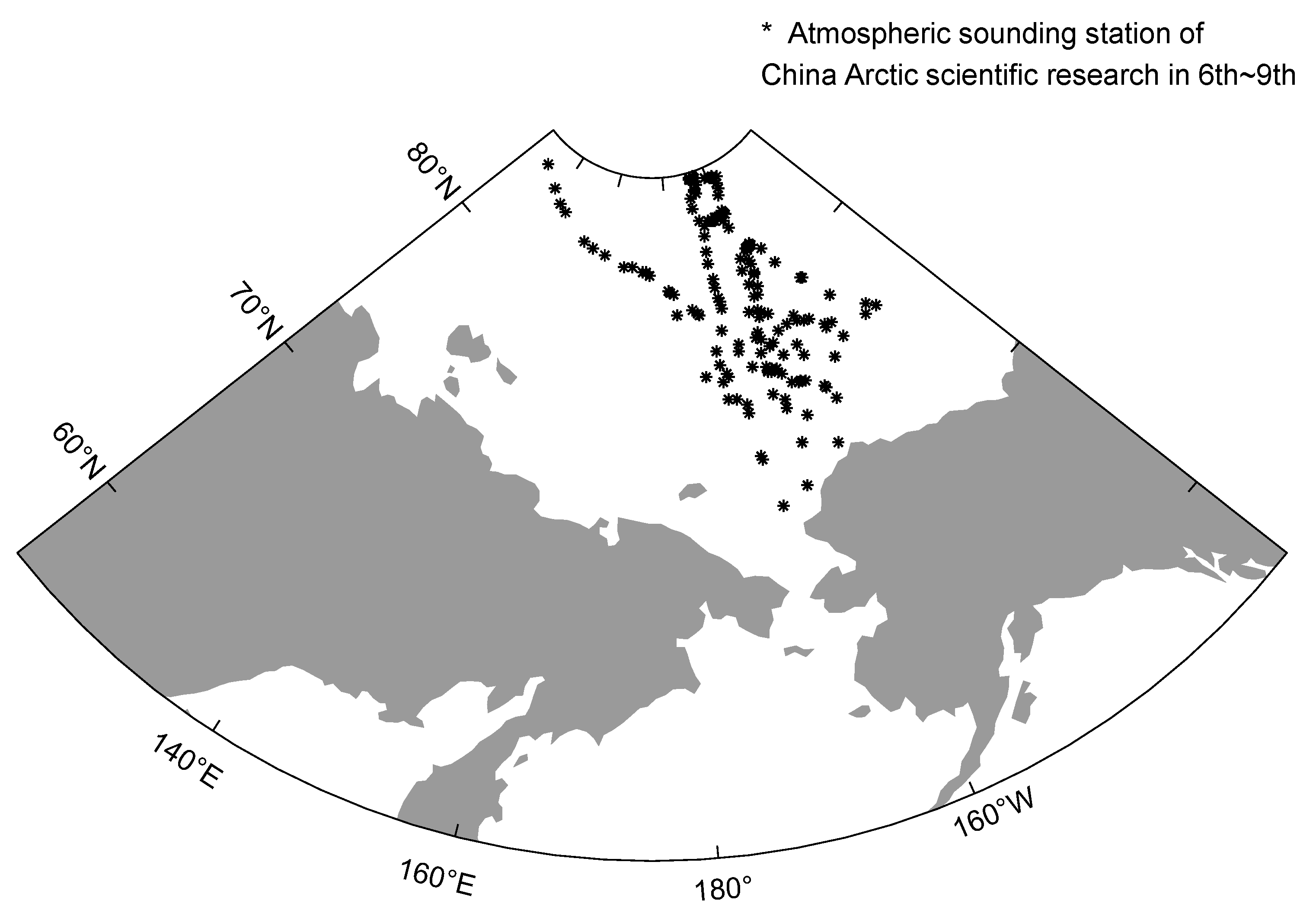
2.1. Data
2.2. Methods
3. Results
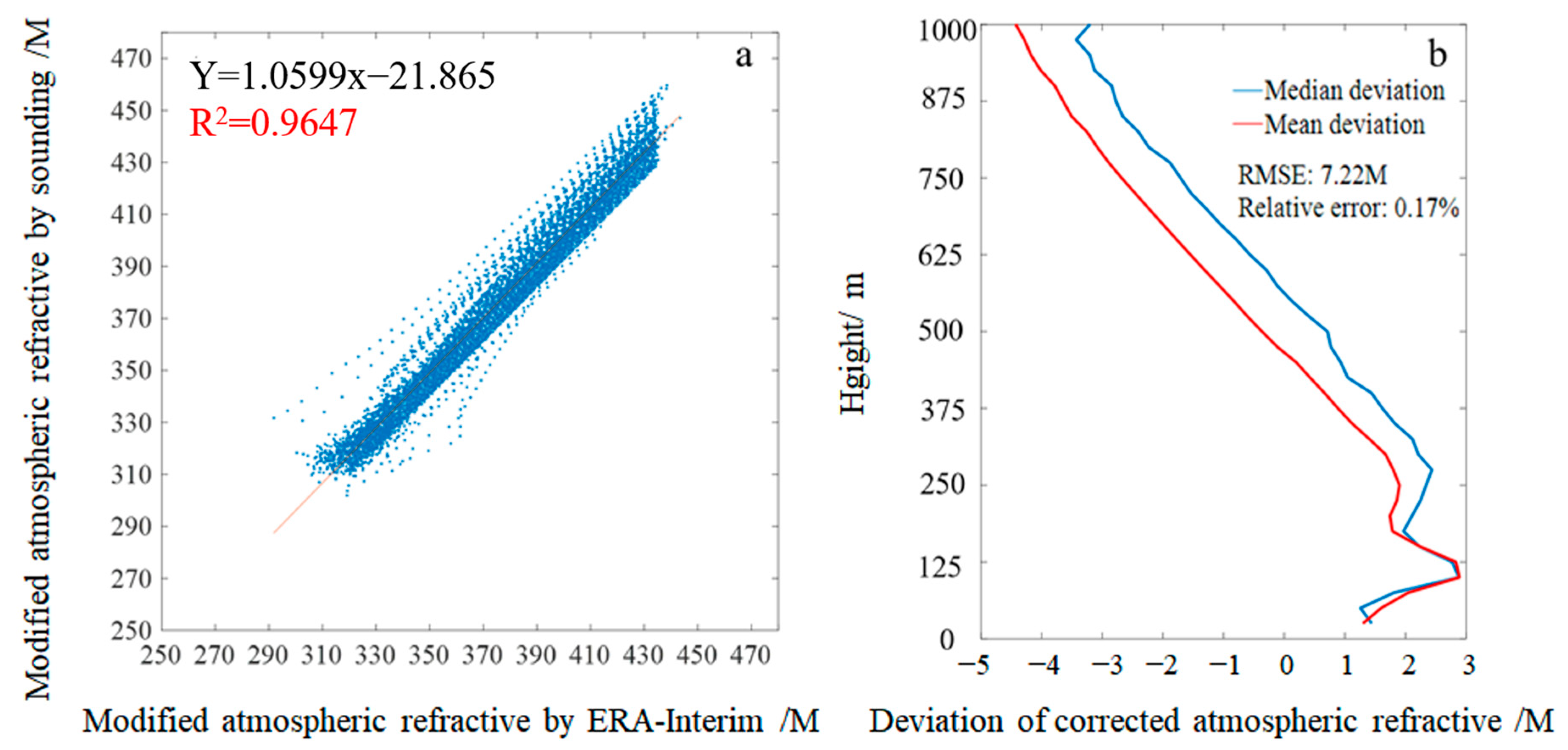
3.1. Comparison of GPS Sounding Observations and Reanalysis Data in the Arctic
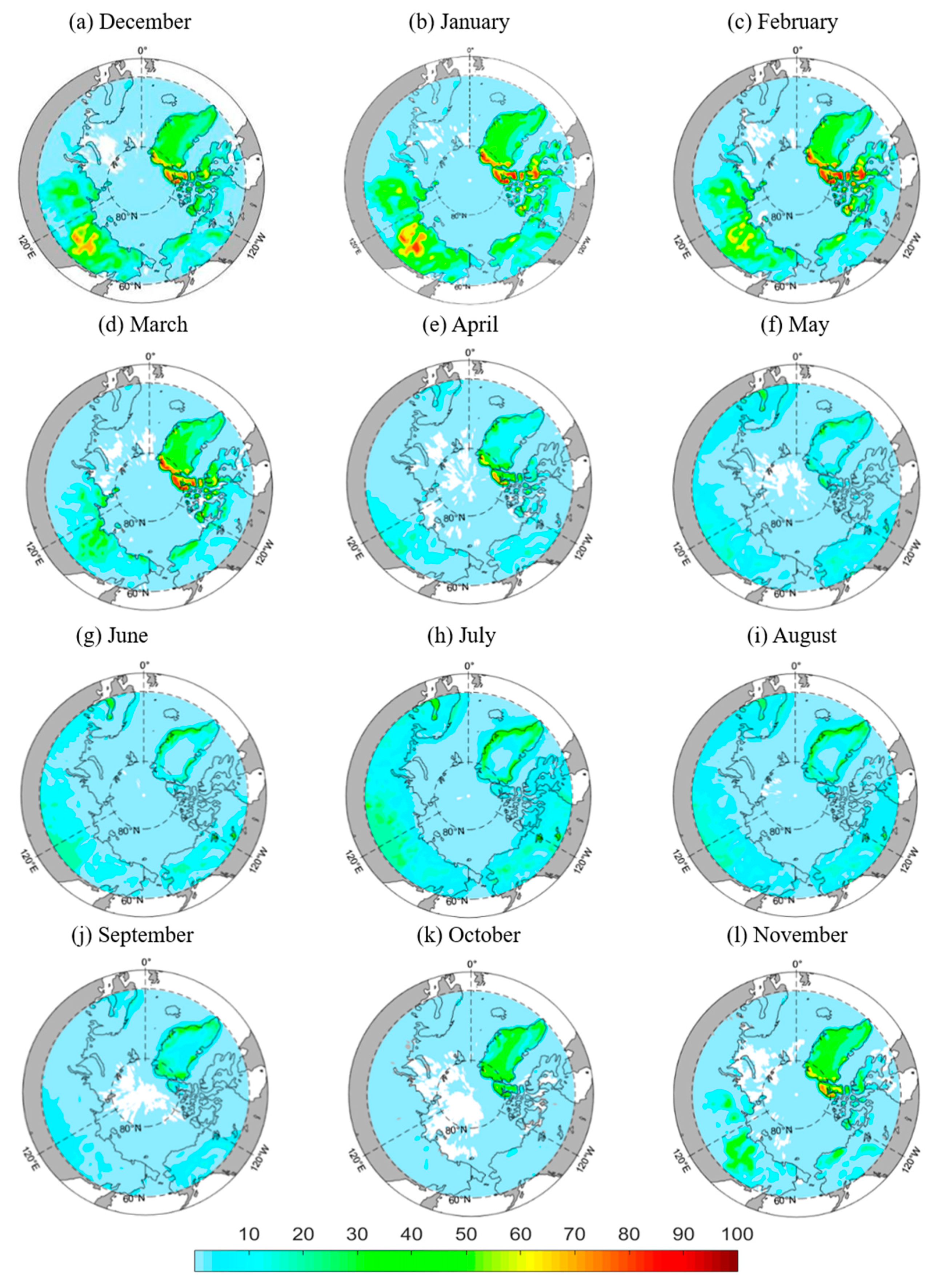
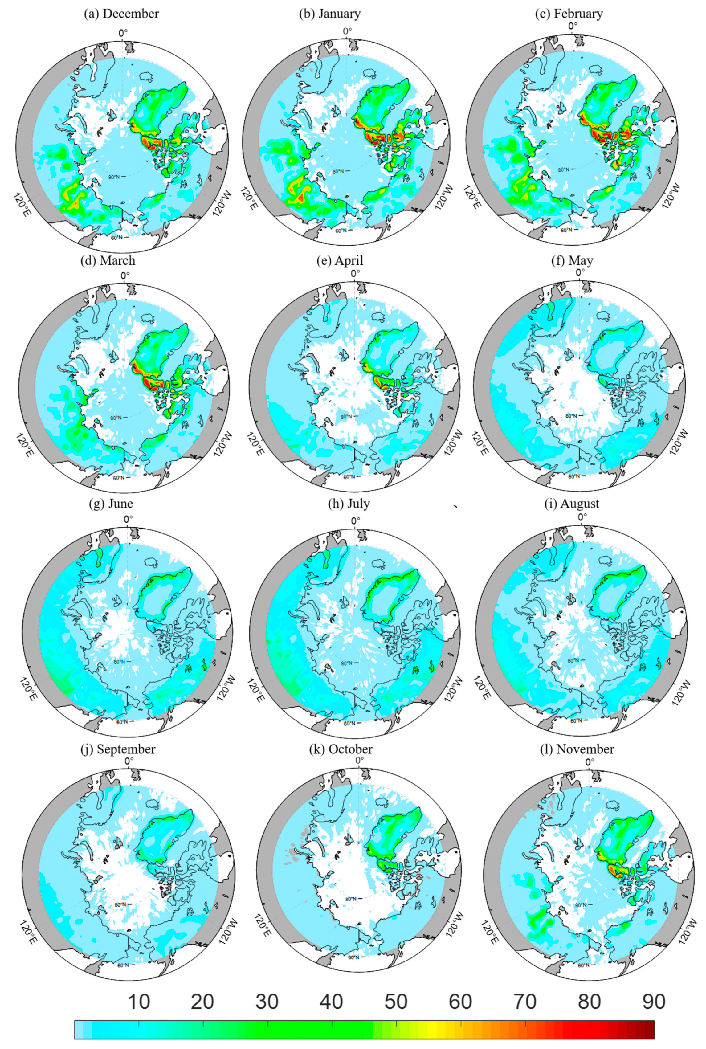
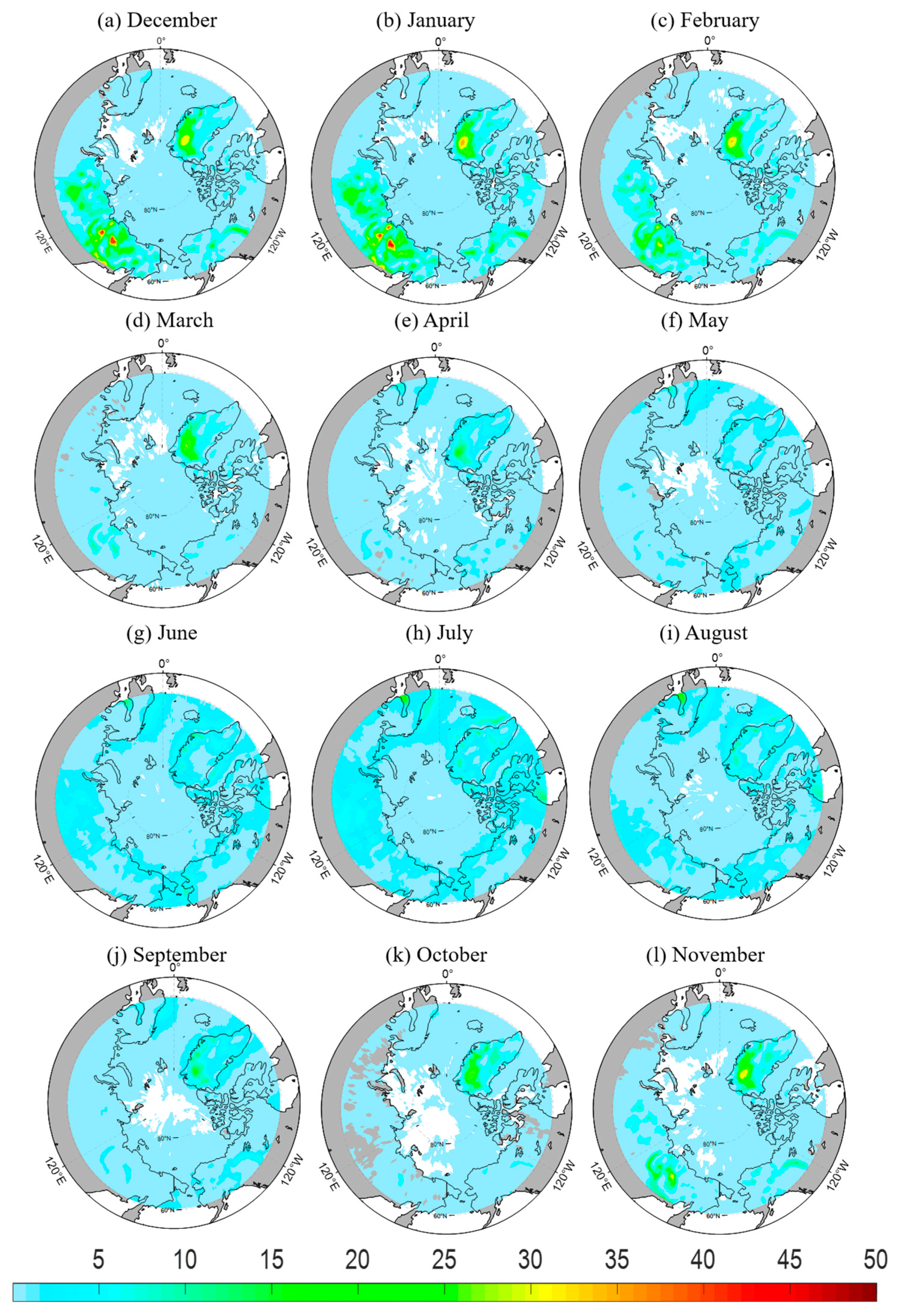
3.2. Spatial Characteristics of Atmospheric Duct Frequencies
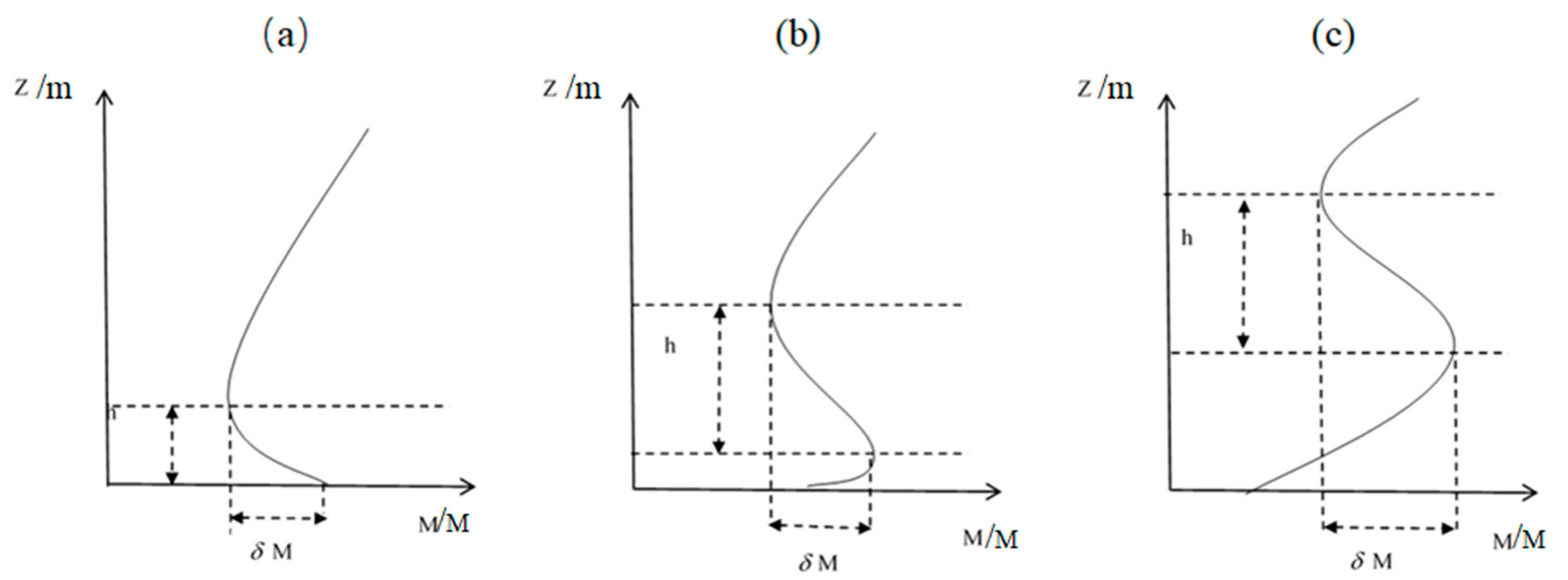
3.3. Height and Intensity Characteristics of Atmospheric Ducts
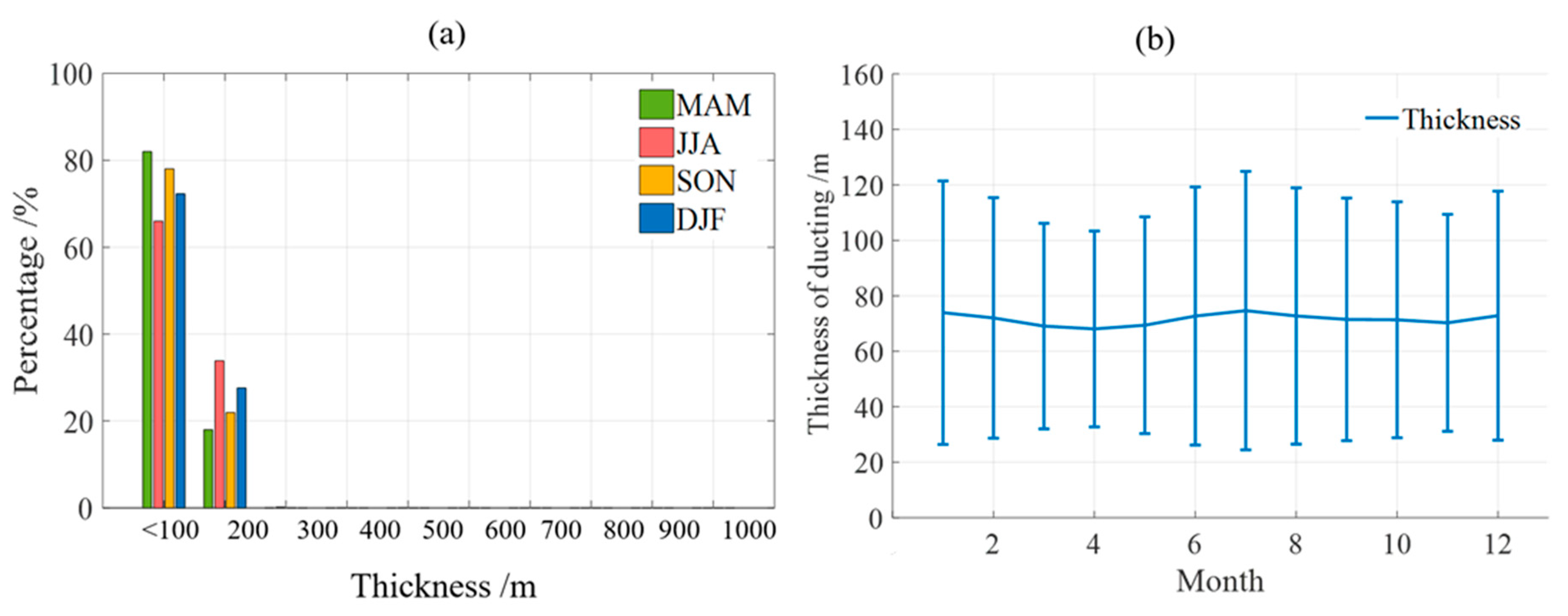
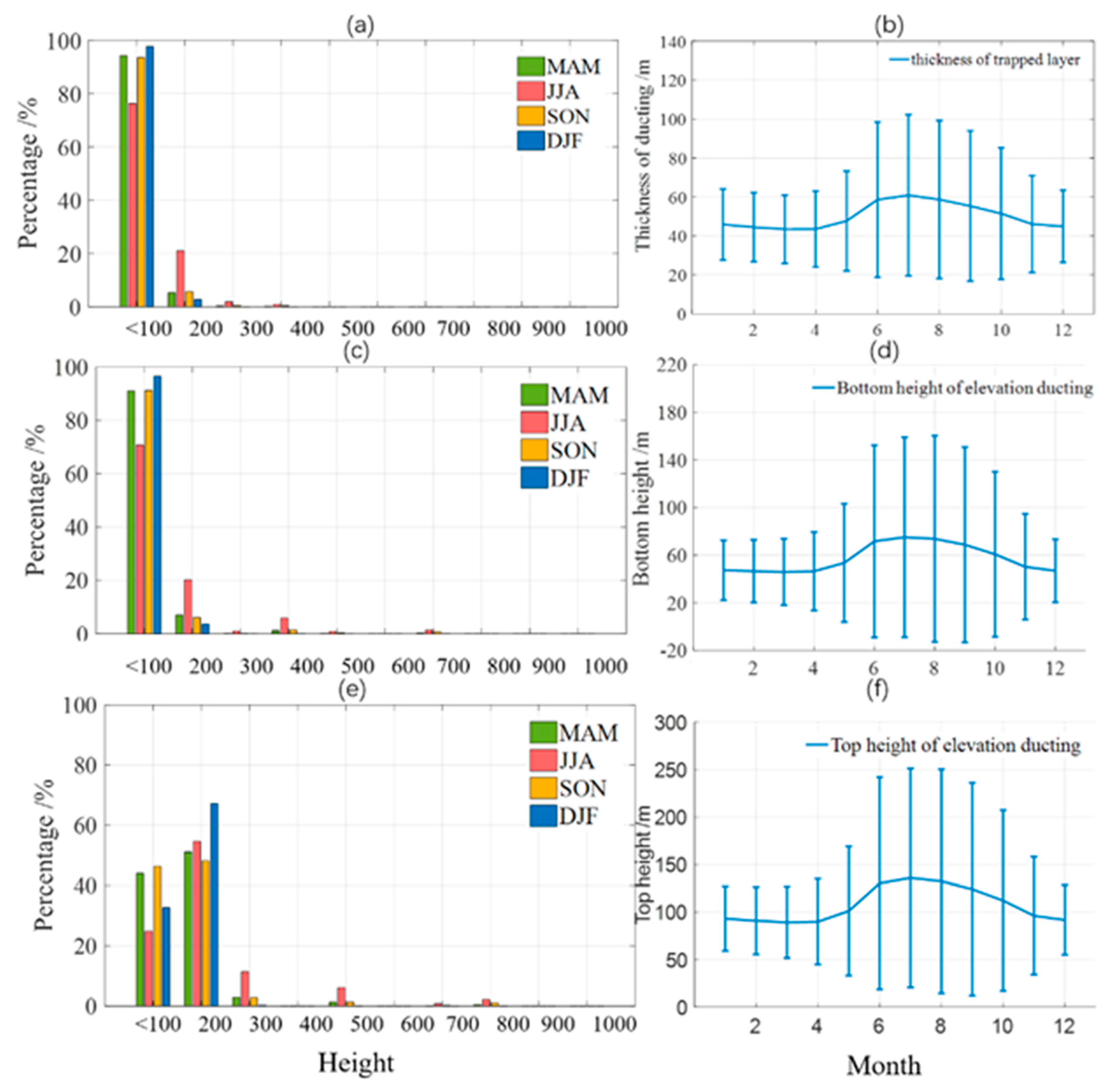
3.3.1. Height Characteristics of Atmospheric Ducts
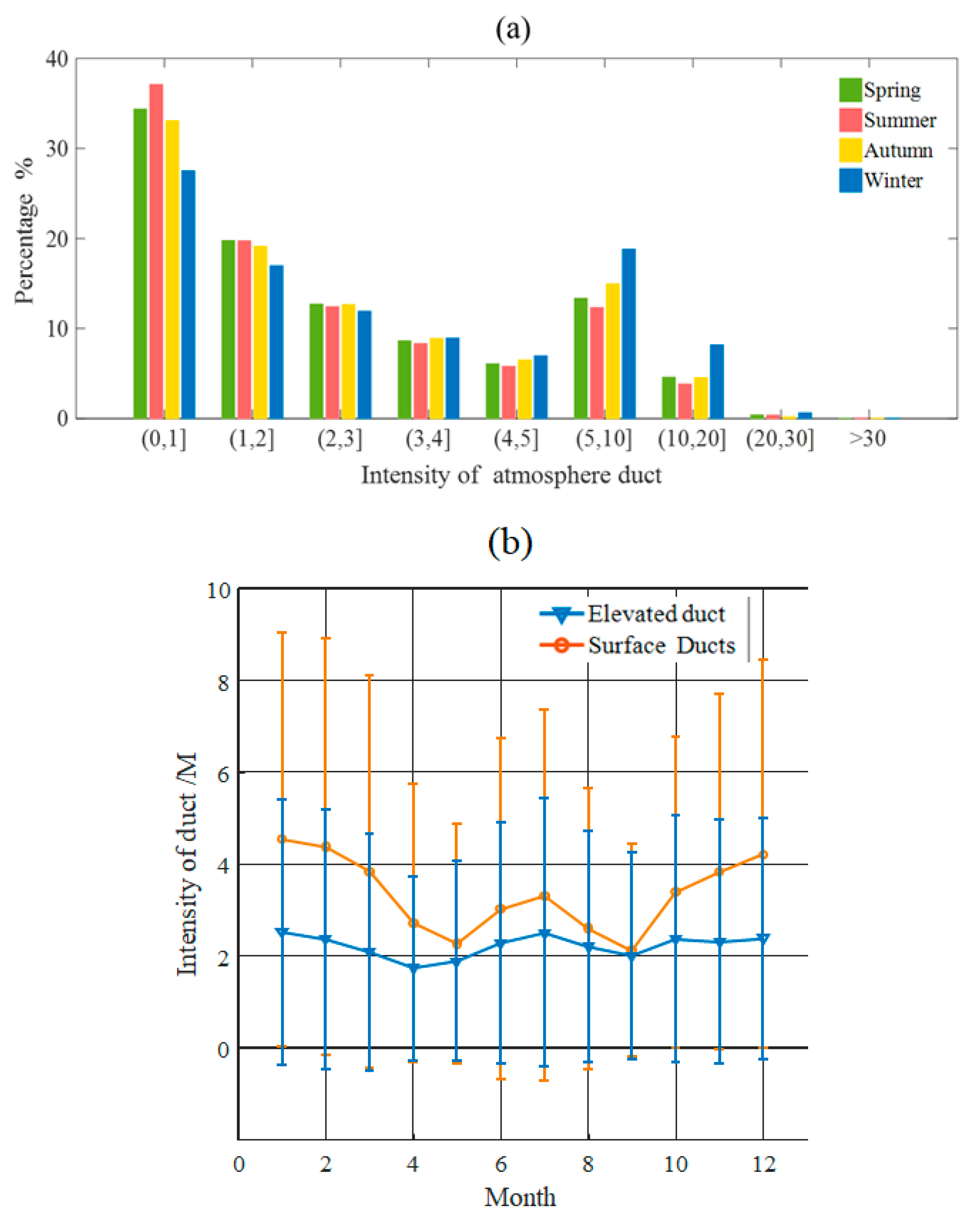
3.3.2. Statistics of Atmospheric Duct Intensities
3.3.3. Correlation between Atmospheric Duct Intensity and Trapped Layer Thickness
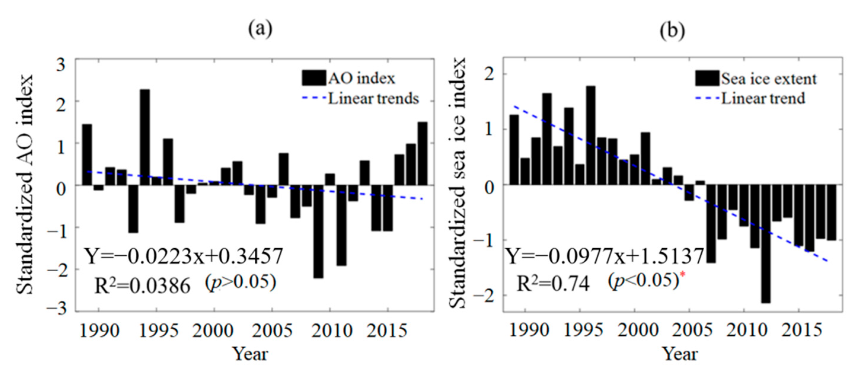
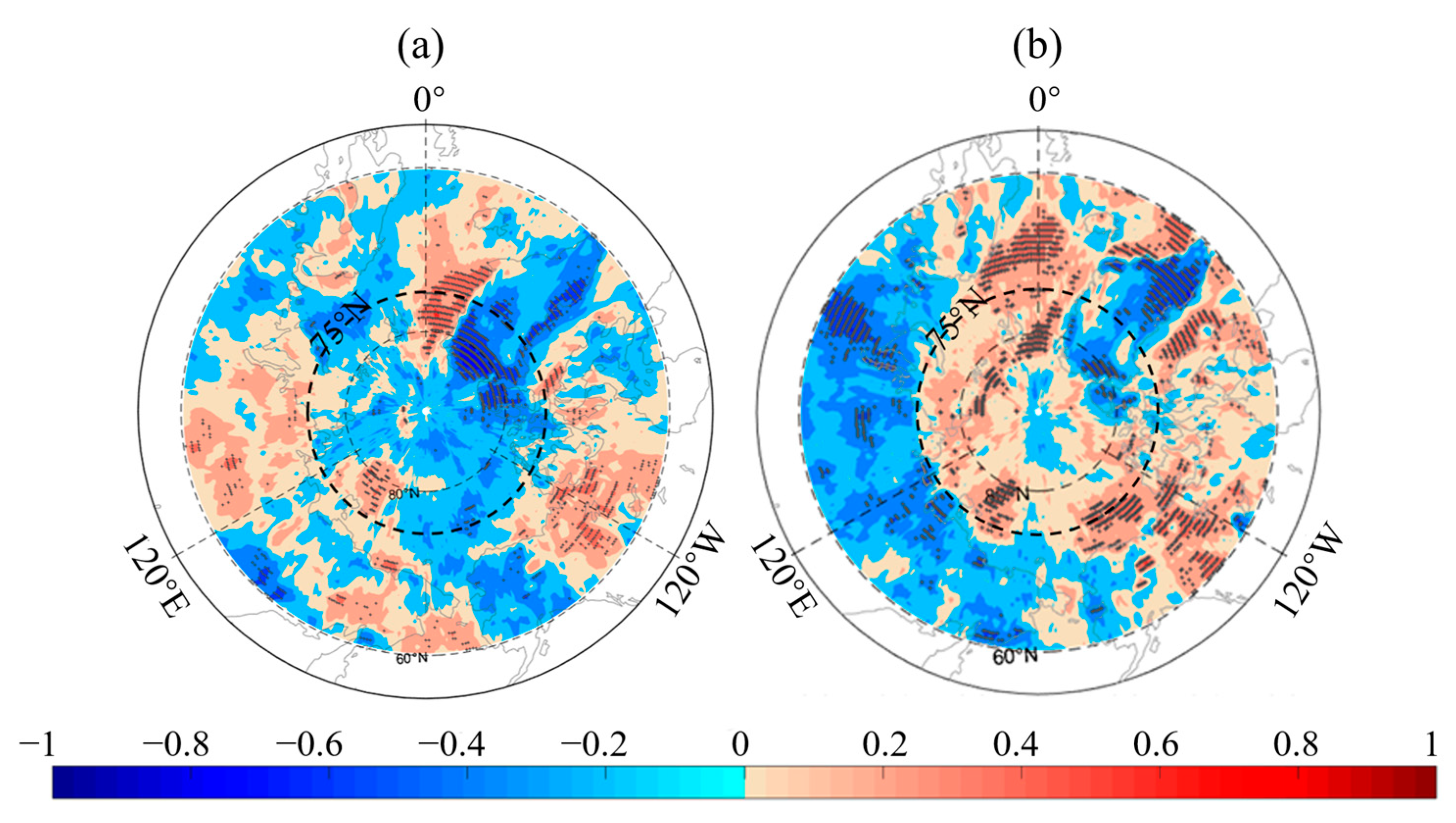
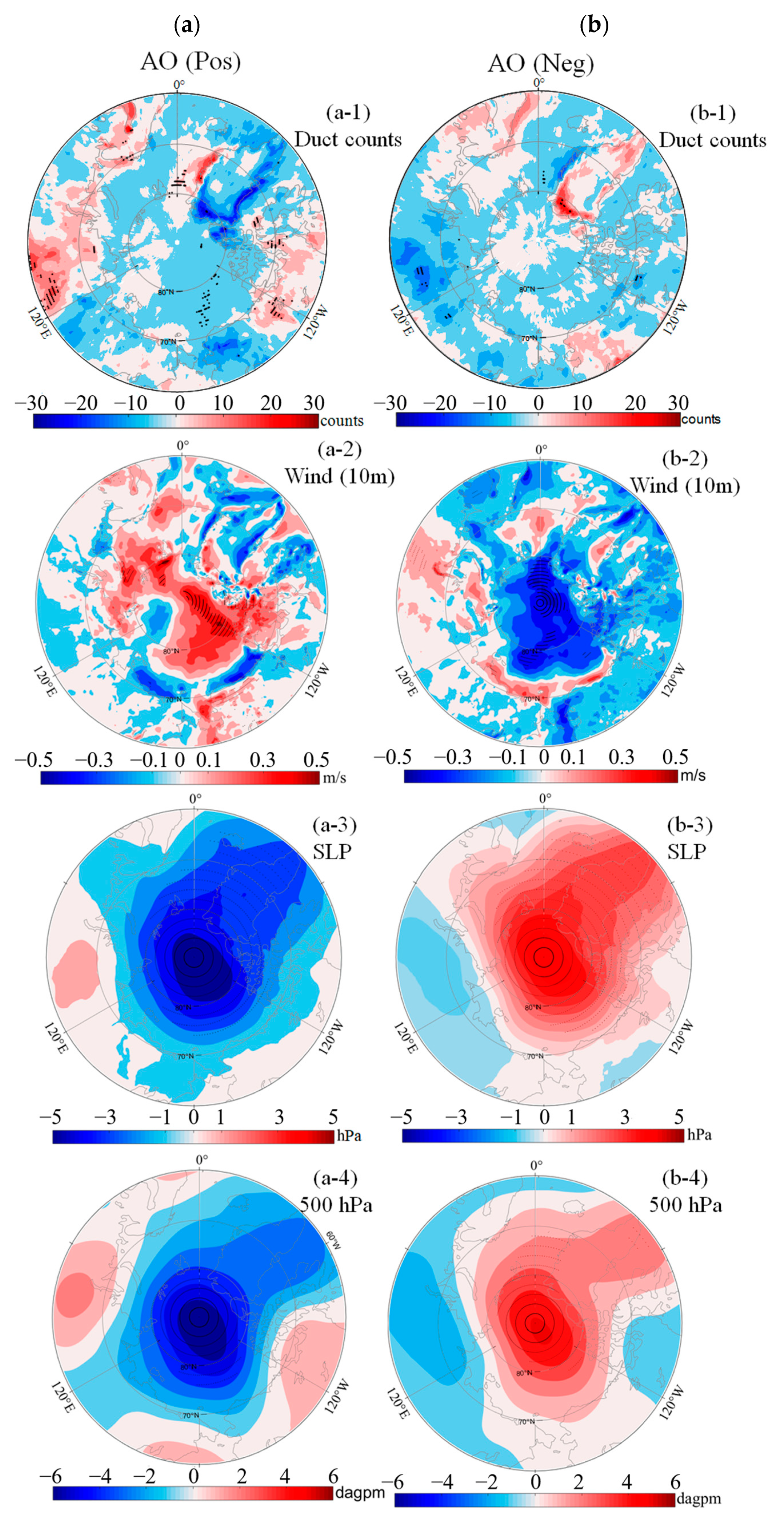
3.4. Response of Atmospheric Ducts to AO and Sea Ice Extent
4. Conclusions and Discussions
Author Contributions
Funding
Institutional Review Board Statement
Informed Consent Statement
Data Availability Statement
Acknowledgments
Conflicts of Interest
References
- Serreze, M.C.; Barry, R.G. Processes and impacts of Arctic amplification: A research synthesis. Glob. Planet. 2011, 77, 85–96. [Google Scholar] [CrossRef]
- Sporyshev, P.V.; Kattsov, V.M.; Gulev, S.K. Changes in surface temperature in the Arctic: Reliability of model reproduction and probabilistic forecast for the near future. Dokl. Earth Sci. 2018, 479, 503–506. [Google Scholar] [CrossRef]
- Aksenov, Y.; Popova, E.E.; Yool, A.; Nurser, A.G.; Williams, T.D.; Bertino, L.; Bergh, J. On the future navigability of Arctic sea routes: High-resolution projections of the Arctic Ocean and sea ice. Mar. Policy. 2017, 75, 300–317. [Google Scholar] [CrossRef] [Green Version]
- Oh, J.; Yang, S.; Lee, B.L. Future projections of ship accessibility for the Arctic Ocean based on IPCC CO2 emission scenarios. Asia-Pac. J. Atmos. Sci. Vol. 2017, 53, 43–50. [Google Scholar] [CrossRef]
- Pustovalov, K.N.; Kharyutkina, E.V.; Korolkov, V.A.; Nagorskiy, P.M. Variations in Resources of Solar and Wind Energy in the Russian Sector of the Arctic. Atmos. Ocean. Opt. 2020, 33, 282–288. [Google Scholar] [CrossRef]
- Zuev, V.V.; Savelieva, E.S.; Pavlinsky, A.V. Features of Stratospheric Polar Vortex Weakening Prior to Breakdown. Atmos. Ocean. Opt. 2022, 35, 183–186. [Google Scholar] [CrossRef]
- Kovadlo, P.G.; Shikhovtsev, A.Y.; Yazev, S.A. The Role of Glaciers in the Processes of Climate Warming. Atmos. Ocean. Opt. 2022, 35, 434–438. [Google Scholar] [CrossRef]
- Lopez, P. A 5-yr 40-km-Resolution Global Climatology of Superrefraction for Ground-Based Weather Radars. J. Appl. Meteorol. Clim. 2009, 48, 89–110. [Google Scholar] [CrossRef]
- Patterson, W.L. Climatology of Marine Atmospheric Refractive Effects. A Compendium of the Integrated Refractive Effects Prediction System (IREPS) Historical Summaries; Naval Ocean Systems Center: San Diego, CA, USA, 1982. [Google Scholar]
- Babin, S.M. Surface Duct Height Distributions for Wallops Island, Virginia, 1985–1994. J. Appl. Meteorol. 1996, 35, 86–93. [Google Scholar] [CrossRef]
- Huang, L.; Zhao, X.; Liu, Y. The Statistical Characteristics of Atmospheric Ducts Observed Over Stations in Different Regions of American Mainland Based on High-Resolution GPS Radiosonde Soundings. Front. Environ. Sci. 2022, 10, 946226. [Google Scholar] [CrossRef]
- Mai, Y.; Sheng, Z.; Shi, H.; Liao, Q.; Zhang, W. Spatiotemporal Distribution of Atmospheric Ducts in Alaska and Its Relationship with the Arctic Vortex. Int. J. Antennas Propag. 2020, 2020, 9673289. [Google Scholar] [CrossRef]
- Liu, C.G.; Huang, J.Y.; Jiang, C.Y. The appearance of the atmospheric ducts structure in the troposphere over the southeast coast. Chin. J. Radio Sci. 2002, 17, 509–513. (In Chinese) [Google Scholar]
- Ding, J.; Fei, J.; Huang, X.; Cheng, X.; Hu, X. Observational occurrence of tropical cyclone ducts from GPS dropsonde data. J. Appl. Meteorol. Climatol. 2013, 52, 1221–1236. [Google Scholar] [CrossRef]
- Cheng, G.; Gao, Z.; Zheng, Y.; Dai, C.; Zhou, M. A Study on Low-level Jets and Temperature Inversion over the Arctic Ocean by Using SHEBA Data. Clim. Environ. Res. 2013, 18, 23–31. (In Chinese) [Google Scholar]
- Cheng, Y.H.; Zhao, Z.W.; Zhang, Y.S. Statistical analysis of low-altitude atmospheric ducts over the South China Sea during monsoon. Chin. J. Radio Sci. 2012, 27, 268–274. (In Chinese) [Google Scholar]
- Chen, L.; Gao, S.H.; Kang, S.F.; Zhang, Y.S.; Wu, Z.M. Statistical analysis on spatial-temporal features of atmospheric ducts over chinese regional seas. Chin. J. Radio Sci. 2009, 24, 702–708. [Google Scholar]
- Cheng, Y.H.; Yang, X.K.; Zhang, Y.S. Characteristics over the China sea based on ECMWF reanalysis data. Oceanol. Limnol. Sin. 2021, 52, 11. (In Chinese) [Google Scholar]
- Wang, H.; Ma, B.; Jiao, L. Study on the distribution of atmospheric ducts based on ECMWF reanalysis data. J. Meteorol. 2021, 79, 521–530. (In Chinese) [Google Scholar] [CrossRef]
- Hao, X.J.; Li, Q.L.; Guo, L.X. Spatial and temporal characteristics of the atmosphere ducts over the North Pole. Chin. J. Polar Res. 2018, 30, 349. (In Chinese) [Google Scholar]
- Von Engeln, A. A ducting climatology derived from the European Centre for Medium-Range Weather Forecasts global analysis fields. J. Geophys. Res. Atmos. 2004, 109, D18104. [Google Scholar] [CrossRef]
- Mentes, S.; Kaymaz, Z. Investigation of Surface Duct Conditions over Istanbul, Turkey. J. Appl. Meteorol. Clim. 2007, 46, 318–337. [Google Scholar] [CrossRef]
- Murthy, N.R.K.; Rao, S.V.B. Study on the occurrence of duct and super-refraction over Indian region. Int. J. Curr. Res. Rev. 2013, 5, 12–20. [Google Scholar]
- Fei, J.; Ding, J.; Huang, X.; Cheng, X.; Hu, X. Numerical study on the impacts of the bogus data assimilation and sea spray parameterization on typhoon ducts. J. Meteorol. Res. 2013, 27, 308–321. [Google Scholar] [CrossRef]
- Liang, Z.; Ding, J.; Fei, J.; Cheng, X.; Huang, X. Maintenance and Sudden Change of a Strong Elevated Ducting Event Associated with High Pressure and Marine Low-Level Jet. J. Meteorol. Res. 2020, 34, 1287–1298. [Google Scholar] [CrossRef]
- Manjula, G.; Raman, M.R.; Ratnam, M.V.; Chandrasekhar, A.V.; Rao, S.V.B. Diurnal variation of ducts observed over a tropical station, Gadanki, using high-resolution GPS radiosonde observations. Radio Sci. 2016, 51, 247–258. [Google Scholar] [CrossRef]
- Wei, L.; Peitao, Z.; Qiyun, G.; Mian, W. The international radiosonde intercomparison results for China-made GPS radiosonde. J. Appl. Meteorol. Sci. 2011, 22, 453–462. [Google Scholar]
- Dee, D.P.; Uppala, S. Variational bias correction of satellite radiance data in the ERA-Interim reanalysis. Q. J. R. Meteorol. Soc. 2009, 135, 1830–1841. [Google Scholar] [CrossRef]
- Graham, R.M.; Hudson, S.R.; Maturilli, M. Improved performance of ERA5 in Arctic gateway relative to four global atmospheric reanalysis. Geophys. Res. Lett. 2019, 46, 6138–6147. [Google Scholar] [CrossRef]
- Bromwich, D.H.; Wilson, A.B.; Bai, L.S.; Moore, G.W.; Bauer, P. A comparison of the regional Arctic System Reanalysis and the global ERA—Interim Reanalysis for the Arctic. Q. J. R. Meteorol. Soc. 2016, 142, 644–658. [Google Scholar] [CrossRef] [Green Version]
- Dee, D.P.; Uppala, S.M.; Simmons, A.J.; Berrisford, P.; Poli, P.; Kobayashi, S.; Andrae, U.; Balmaseda, M.A.; Balsamo, G.; Bauer, P.; et al. The ERA-Interim reanalysis: Configuration and performance of the data assimilation system. Q. J. R. Meteorol. Soc. 2011, 137, 553–597. [Google Scholar] [CrossRef]
- Berrisford, P.; Dee, D.; Poli, P.; Brugge, R.; Fielding, K.; Fuentes, M.; Kallberg, P.; Kobayashi, S.; Uppala, S.; Simmons, A. The ERA-Interim Archive Version 2.0. ERA Report Series 1. 2011. Available online: http://www.ecmwf.int/en/elibrary/8174-era-interim-archive-version-20 (accessed on 2 October 2022).
- Thompson, D.W.J.; Wallace, J.M. Annular modes in the extratropical circulation. Part I: Monthto-month variability. J. Clim. 2000, 13, 1000–1016. [Google Scholar] [CrossRef]
- Hersbach, H.; Bell, B.; Berrisford, P.; Biavati, G.; Horányi, A.; Muñoz Sabater, J. ERA5 monthly averaged data on single levels from 1959 to present. Copernicus Climate Change Service (C3S). Clim. Data Store 2019, 10, 252–266. [Google Scholar]
- Tian, Z.; Zhang, D.; Song, X.; Zhao, F.; Li, Z.; Zhang, L. Characteristics of the atmospheric vertical structure with different sea ice covers over the Pacific sector of the Arctic Ocean in summer. Atmos. Res. 2020, 245, 105074. [Google Scholar] [CrossRef]
- Xie, Q.; Huang, K.; Wang, D.; Yang, L.; Chen, J.; Wu, Z.; Li, D.; Liang, Z. An inter-comparison of GPS radiosonde soundings during the eastern tropical Indian Ocean experiment. Acta Oceanol. Sin. 2014, 33, 127–134. [Google Scholar] [CrossRef]
- Bean, B.R.; Dutton, E.J. Radio Meteorology; Dover: New York, NY, USA, 1968; 435p. [Google Scholar]
- Lee, W.; Song, I.; Kim, J.; Kim, Y.H.; Jeong, S.; Eswaraiah, S.; Murphy, D.J. The Observation and SD-WACCM Simulation of Planetary Wave Activity in the Middle Atmosphere During the 2019 Southern Hemispheric Sudden Stratospheric Warming. J. Geophys. Res. Space Phys. 2021, 126, e2020JA029094. [Google Scholar] [CrossRef]
- Rogers, R.R.; Yau, M.K. A Short Course in Cloud Physics, 3rd ed.; Pergamon Press: London, UK, 1989. [Google Scholar]
- Bolton, D. The Computation of Equivalent Potential Temperature. Mon. Weather Rev. 1980, 108, 1046–1053. [Google Scholar] [CrossRef]
- Liu, J.W.; Guo, H.; Li, Y.D. Basic Calculation of Physical Quantities for Weather Analysis and Forecast; China Meteorological Press: Beijing, China, 2005. (In Chinese) [Google Scholar]
- Turton, J.D.; Bennetts, D.A.; Farmer, S.F.G. An introduction to radio Ducting. Meteor Mags 1988, 117, 245–254. [Google Scholar]
- Ruman, C.J.; Monahan, A.H.; Sushama, L. Climatology of Arctic temperature inversions in current and future climates. Theory Appl. Climatol. 2022, 150, 121–134. [Google Scholar] [CrossRef]
- Shikhovtsev, A.Y.; Bolbasova, L.A.; Kovadlo, P.G.; Kiselev, A.V. Atmospheric parameters at the 6-m Big Telescope Alt-azimuthal site. Mon. Not. R. Astron. Soc. 2020, 493, 723–729. [Google Scholar] [CrossRef]
- Wei, L.X.; Qin, T.; Li, C. Seasonal and inter-annual variations of Arctic cyclones and their linkage with Arctic sea ice and atmospheric teleconnections. Acta Oceanol. Sin. 2017, 10, 5–11. [Google Scholar] [CrossRef]


| Parameter | Total Ducts/% | Surface Ducts/% | Elevated Ducts/% | |||||||||
|---|---|---|---|---|---|---|---|---|---|---|---|---|
| Latitude | Spr. | Sum. | Aut. | Win. | Spr. | Sum. | Aut. | Win. | Spr. | Sum. | Aut. | Win. |
| 60° N–70° N | 7.1 | 10.2 | 4.4 | 12.9 | 5.9 | 7.4 | 2.9 | 8.8 | 1.2 | 2.9 | 1.5 | 4.0 |
| 70° N–80° N | 5.7 | 3.8 | 4.9 | 11.8 | 4.5 | 2.0 | 3.3 | 8.8 | 1.3 | 1.8 | 1.6 | 2.9 |
| 80° N–90° N | 3.1 | 1.2 | 2.7 | 5.0 | 2.6 | 0.6 | 2.1 | 4.0 | 0.5 | 0.6 | 0.5 | 1.0 |
| Total | 5.3 | 5.1 | 4.0 | 9.9 | 4.3 | 3.3 | 2.8 | 7.3 | 1.0 | 1.8 | 1.2 | 2.7 |
| Month | Correlation Coefficient (Surface) | Confidence Interval | Correlation Coefficient (Elevated) | Confidence Interval |
|---|---|---|---|---|
| 1 | 0.230 * | 0.229–0.231 | 0.256 * | 0.254–0.257 |
| 0.228 * | 0.227–0.229 | 0.253 * | 0.252–0.254 | |
| 3 | 0.232 * | 0.231–0.233 | 0.246 * | 0.245–0.247 |
| 4 | 0.234 * | 0.233–0.234 | 0.243 * | 0.241–0.244 |
| 5 | 0.263 * | 0.262–0.263 | 0.203 * | 0.202–0.204 |
| 6 | 0.315 * | 0.314–0.315 | 0.201 * | 0.200–0.202 |
| 7 | 0.338 * | 0.337–0.339 | 0.249 * | 0.247–0.250 |
| 8 | 0.310 * | 0.309–0.311 | 0.232 * | 0.230–0.233 |
| 9 | 0.298 * | 0.297–0.299 | 0.231 * | 0.299–0.232 |
| 10 | 0.273 * | 0.272~0.274 | 0.210 * | 0.209–0.211 |
| 11 | 0.220 * | 0.219–0.221 | 0.216 * | 0.215–0.217 |
| 12 | 0.227 * | 0.226–0.227 | 0.244 * | 0.243–0.245 |
| Positive AO anomaly years | 1989, 1994, 1996, 2006, 2016, 2017, 2018 |
| Negative AO anomaly years | 1993, 1997, 2004, 2007, 2009, 2011, 2014, 2015 |
Publisher’s Note: MDPI stays neutral with regard to jurisdictional claims in published maps and institutional affiliations. |
© 2022 by the authors. Licensee MDPI, Basel, Switzerland. This article is an open access article distributed under the terms and conditions of the Creative Commons Attribution (CC BY) license (https://creativecommons.org/licenses/by/4.0/).
Share and Cite
Qin, T.; Su, B.; Chen, L.; Yang, J.; Sun, H.; Ma, J.; Yu, W. Arctic Atmospheric Ducting Characteristics and Their Connections with Arctic Oscillation and Sea Ice. Atmosphere 2022, 13, 2119. https://doi.org/10.3390/atmos13122119
Qin T, Su B, Chen L, Yang J, Sun H, Ma J, Yu W. Arctic Atmospheric Ducting Characteristics and Their Connections with Arctic Oscillation and Sea Ice. Atmosphere. 2022; 13(12):2119. https://doi.org/10.3390/atmos13122119
Chicago/Turabian StyleQin, Ting, Bo Su, Li Chen, Junfeng Yang, Hulin Sun, Jing Ma, and Wenhao Yu. 2022. "Arctic Atmospheric Ducting Characteristics and Their Connections with Arctic Oscillation and Sea Ice" Atmosphere 13, no. 12: 2119. https://doi.org/10.3390/atmos13122119